Shot noise in a diffusive F-N-F spin valve
Abstract
Fluctuations of electric current in a spin valve consisting of a diffusive conductor connected to ferromagnetic leads and operated in the giant magnetoresistance regime are studied. It is shown that a new source of fluctuations due to spin-flip scattering enhances strongly shot noise up to a point where the Fano factor approaches the full Poissonian value.
pacs:
72.70.+m, 72.25.-b, 75.47.DeTransport in various spintronic devices ALS containing ferromagnet-paramagnet interfaces is attracting a lot of attention. Considerable experimental and theoretical efforts have been directed towards the understanding of magnetoresistance, spin injection, spin accumulation, spin-orbit interaction, current-induced torque and other fascinating and challenging effects (the vast and quickly expanding bibliography is far beyond the scope of this Letter). Advances in technology and sample fabrication resulting in devices of nanoscale dimensions led the methods and notions of spintronics to be the natural outgrows and further developments of the exciting and successful ideas of mesoscopics.
One of the issues outstanding in mesoscopic physics has been the phenomenon of the shot noise, i.e. current fluctuations in nonequilibrium conductors BlB . In particular, an experimental confirmation SMD of the theoretically predicted -suppression (compared to the Poissonan value characteristic for the transmission of independent particles) of the noise signal in diffusive conductors BB ; Nag is one of the milestones in the field. Shot noise in ferromagnet-normal metal constrictions is also evolving into a subject of much interest. Current fluctuations in a F-quantum dot-F system in the Coulomb blockade regime were considered in Refs. BMM ; Bul ; LL ; SEJ , noise in a quantum dot in the Kondo regime analyzed in Ref. LS , ballistic beam splitter with spin-orbit interaction discussed in Ref. EBL . Dependence of the shot noise in a diffusive conductor attached to ferromagnetic reservoirs on the relative angle between the magnetizations of reservoirs has been studied in Ref. TB with the help of the circuit theory BNB . However, effects of a spin-flip scattering on the fluctuations of electric current in diffusive conductors have been disregarded so far. In the present Letter we show them to make a profound effect on the shot noise power.
The universal -shot noise in a conventional diffusive conductor is due to the interplay of the random impurity scattering and restrictions imposed by the Fermi statistics. In the presence of ferromagnetic contacts, however, the spin degeneracy is lifted with spin-up and spin-down electrons representing two different subsystems. The number of particles in each subsystem is not conserved (due to spin-flip scattering) leading therefore to a new class of fluctuations. The situation here resembles closely the fluctuations of radiation in random optical media Ben . The absence of particle conservation in a gas of photons results in the enhancement of photon flux noise above the Poissonian value (also the result of bunching typical for bosons). With the notable difference in statistics (Fermi instead of Bose) the framework of stochastic diffusion equations MB ; MPB can be formulated for the fluctuations in disordered spintronic devices as well.

To demonstrate this we discuss the most characteristic example of a spin valve in the giant magnetoresistance regime, when the transport across the valve is extremely sensitive to the intensity of a spin-flip scattering. Namely, we consider a diffusive paramagnetic conductor (N) sandwiched between two ideal ferromagnetic (F) leads, Fig. 1. ’Ideal’ means that electron distributions inside the leads are not affected by the presence of the normal region (a typical mesoscopic setup assuming the conduction and screening in the leads to be more efficient than in the conductor). In addition, we assume that conduction electrons are completely polarized inside the ferromagnets, i.e. the population of carriers with a spin direction opposite to that of a magnet is fully depleted (half-metallic ferromagnets). Therefore, when the polarizations of the leads are antiparallel, a conduction electron cannot be transferred across the valve without changing its spin direction. As a result the resistance of a spin-filter is very large unless there is a substantial amount of spin-flip scattering inside the N-region. We assume the F-N interfaces to be spin-conserving but allow for the finite contact (tunnel) resistances .
Stochastic diffusion equations. The electron motion inside the N-region is diffusive with the mean free path much smaller than the size of the valve (but yet much larger than the Fermi wavelength). At temperatures low enough the inelastic (electron-phonon, electron-electron) scattering is suppressed (once the inelastic scattering length exceeds ). The electron distribution is therefore almost isotropic in momentum space and can be described by the spin and energy-dependent distribution functions , with being a spin index: corresponding to spin-up electrons and to spin-down electrons.
If the system is driven out of equilibrium (e.g. by applying a voltage bias to the leads), the distribution function becomes spatially inhomogeneous resulting in the electric current (we assume the cross-sectional area of the valve to be equal to unity),
| (1) |
where is the conductivity in the N-region, is the density of states per single spin direction and is the diffusion constant. The last term in Eq. (1) is the stochastic Langevin source. It has zero expectation value and a correlator that similarly to the spinless case Nag is determined by the mean value of the electron distribution function,
where we have abbreviated and assumed no summation over the repeated indexes. The stochastic source is due to the random independent (i.e. Poissonian) events of spin-conserving scattering from disorder.
The particle conservation implies a second relation between the electric current and particle density (hereinafter we drop the arguments when it could not lead to confusion),
| (2) |
The first term in the right-hand side accounts for the average particle flow between states with opposite spins due to spin-flip scattering (customary in treating spin-dependent diffusion problems SKW ). The spin-flip length is assumed to be much larger than the mean free path but no restrictions as to its relation to the size of the system are imposed. The last term in Eq. (2) is the Langevin source for the spin-flip scattering arising from randomness of a spin-flip process. It is similar to the stochastic terms for the fluctuations of the number of photons in disordered optical media MB . Its second moment is equal to the mean flow between states with different spin directions,
| (3) |
which utilizes the fact that spin-flip scattering events are independent and obey Poissonian statistics. In writing Eqs. (2-3) we suggested that the spin-flip scattering is energy-conserving. This assumption is well justified whenever a typical energy change during a spin-flip is small compared to the characteristic scale of the electron distribution (set by the temperature or external bias ).
The above equations must be supplemented with appropriate boundary conditions. We assume that the interface resistances at the left and right contacts are the same . Since there is no charge accumulation in the system, the diffusive currents (1) should match the tunneling currents through the interfaces. In particular, for the antiparallel valve configuration the boundary conditions read,
| (4) |
For the parallel configuration one has to interchange and indexes in the second line of Eq. (4). The stochastic sources and accounting for the randomness of the electron tunneling through the interfaces have (at ) the variance t ,
| (5) |
here is the total current independent of the coordinate , as readily seen from Eq. (2). The current at the contacts is due to electrons with a single spin direction only.
It is convenient to use the particle density and spin density distributions as well as the corresponding Langevin sources,
Combining Eqs. (1) and (2) we obtain (in the stationary regime) the equations for the particle and spin distribution,
| (6) |
Note, that different Langevin terms () are independent and have zero cross-correlators.
Average electric current. The mean (averaged over time) solution of the equations (6) with the boundary conditions (4) is elementary and yields the distribution function,
| (7) |
with standing for the characteristic resistance on a spin-flip length . The total resistance and the function depend on the magnetization of the leads. For the antiparallel configuration,
| (8) |
while for the parallel configuration,
| (9) |
Here is the dimensionless measure of the amount of spin-flip scattering in the system, and is the resistance of the normal region.
The total mean electric current calculated with the help of Eqs. (1) and (7) is determined by the total resistance,
| (10) |
where the bias is the difference in the chemical potentials of the left and right leads . In the absence of spin-flip scattering the resistance of the parallel (the valve switched ’on’) configuration tends to the value, while for the antiparallel one (the valve switched ’off’) it diverges. For , both resistances tend to .
Shot noise. To solve Eqs. (6) it is convenient to write the fluctuating part of the distribution function in the form,
| (11) | |||||
| (12) | |||||
with the help of the Green function vanishing at the interfaces,
| (13) |
with standing for the smaller (larger) of the two coordinates . The function is determined from the same expression (13) with . The coefficients are to be determined from the boundary conditions (4). It should be pointed out that the distributions in the leads do not fluctuate . The fluctuation of the total current is determined by the coefficient only, according to,
| (14) |
Resolving a set of linear algebraic equations (obtained from the boundary conditions) with respect to we find the fluctuation of the total energy-resolved current,
| (15) | |||||
where the kernel function depends on the valve configuration,
| (16) |
The static shot noise power determined as the zero-frequency transform of the current-current correlation function can now be calculated from Eq. (15) with the help of the correlation functions for the Langevin sources,
| (17) |
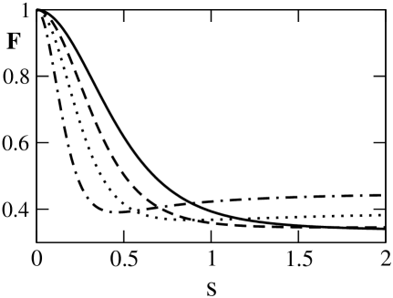
Substituting the mean distribution functions (7) into Eq. (Shot noise in a diffusive F-N-F spin valve) and evaluating the spatial integrals we obtain the final expressions for the dimensionless noise-to-current ratio, , also known as the Fano factor,
| (18) | |||
| (19) |
with being the dimensionless total resistance: for the antiparallel configuration and for the parallel configuration. We also introduced the dimensionless tunneling resistance .
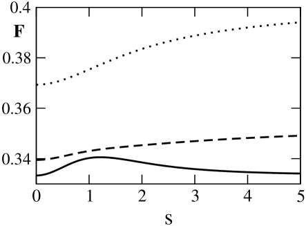
Figs. 2 and 3 illustrate the Fano factor behavior with the spin-flip intensity for different values of the contact resistance for antiparallel and parallel valve configurations respectively. Let us first discuss the regime of transparent F-N interfaces . For large spin-flip scattering, , the shot noise approaches the universal value independent of the relative magnetization of the leads. This is obvious since an injected electron quickly loses its polarization. For intermediate values, , the noise is slightly increased by spin-flip scattering both for parallel and antiparallel spin valve configurations. For small spin-flip intensity, , the noise behavior is completely different. In the parallel configuration the Fano factor is returned to its universal value , which is easy to understand by realizing that electric current is transferred predominantly by the spin-down states. In the antiparallel configuration, however, the small-amount of spin-flip scattering is responsible for the finite conductance itself. The spin-flip induced fluctuations contribute to the noise comparably to the disorder-induced fluctuations. The noise power is therefore enhanced reaching ultimately the full Poissonian value usually reflective of the independent electron transmission, like in a tunnel junction or a Shottky vacuum diode.
The presence of contacts with the finite resistance changes the noise-to-current ratio. For large spin-flip scattering,
the Fano factor is increased monotonously from to by changing from zero to infinity. Exactly opposite, however, happens for antiparallel configuration with low spin-flip scattering (’off’-state of the valve), , where the presence of contacts actually suppresses the noise power.
The stochastic diffusion equations presented here allow for the discussion of the time-dependent problems as well, e.g. frequency dependence of the noise power. Without spin-flip scattering the noise spectrum is white as a result of the Debye screening BlB . Shot noise in a spin valve is different since fluctuations of spin density do not require fluctuations of charge density. Mathematically it is illustrated by the existence of the new (spin-flip) frequency scale . The calculations would be similar to those performed for the phononic noise spectrum MPB .
Fruitful discussions with B. Halperin, D. Davidovic and E. Demler are gratefully appreciated. This material is based on work supported by the NSF under grant PHY-01-17795 and by the Defence Advanced Research Programs Agency (DARPA) under Award No. MDA972-01-1-0024.
References
- (1) Semiconductor Spintronics and Quantum Computation, eds. D.D. Awschalom, D. Loss, and N. Samarth (Springer, Berlin, 2002).
- (2) Ya.M. Blanter and M. Büttiker, Phys. Rep. 336, 1 (2000).
- (3) A.H. Steinbach, J.M. Martinis, and M.H. Devoret, Phys. Rev. Lett. 76, 3806 (1996).
- (4) C.W.J. Beenakker and M. Büttiker, Phys. Rev. B 46, 1889 (1992).
- (5) K.E. Nagaev, Phys. Lett. A 169, 103 (1992).
- (6) B.R. Bulka, J. Martinek, G. Michalek and J. Barnas, Phys. Rev. B 60, 12 246 (1999).
- (7) B.R. Bulka, Phys. Rev. B 62, 1186 (2000).
- (8) R. Lu, Z.-R. Liu, preprint, cond-mat/0210350.
- (9) F.M. Souza, J.C. Egues, A.-P. Jauho, preprint, cond-mat/0209263.
- (10) R. Lopez and D. Sanchez, preprint, cond-mat/0302125.
- (11) J.C. Egues, G. Burkard and D. Loss, Phys. Rev. Lett. 89, 176401 (2002).
- (12) Ya. Tserkovnyak and A. Brataas, Phys. Rev. B 64, 214402 (2001).
- (13) A. Brataas, Yu.V. Nazarov, and G.E. Bauer, Phys. Rev. Lett. 84, 2481 (2000); Eur. Phys. J. B 22, 99 (2001).
- (14) C.W.J. Beenakker, in Diffusive Waves in Complex Media, edited by J.-P. Fouque, ATO ASI Ser. C531 (Kluwer, Dordrecht, 1999).
- (15) E.G. Mishchenko and C.W.J. Beenakker, Phys. Rev. Lett. 83, 5475 (1999).
- (16) E.G. Mishchenko, M. Patra and C.W.J. Beenakker, Eur. Phys. J. D 13, 289 (2001).
- (17) P.C. van Son, H. van Kampen, and P. Wyder, Phys. Rev. Lett. 58, 2271 (1987).
- (18) This formula holds for only. To consider the effects of thermal fluctuations one needs a more general expression for the intrinsic noise of a tunnel barrier, , where and are the distribution functions at the left and right side of the barrier.