Spin dynamics from Majorana fermions

Abstract

Using the Majorana fermion representation of spin-$1/2$ local moments, we show how it is possible to directly read off the dynamic spin correlation and susceptibility from the one-particle propagator of the Majorana fermion. We illustrate our method by applying it to the spin dynamics of a non-equilibrium quantum dot, computing the voltage-dependent spin relaxation rate and showing that, at weak coupling, the fluctuation-dissipation relation for the spin of a quantum dot is voltage-dependent. We confirm the voltage-dependent Curie susceptibility recently found by Parcollet and Hooley [Phys. Rev. B 66, 085315 (2002)].

The mathematical difficulties of representing spins in many body physics have long been recognized. The essence of the problem is that spin operators are non-abelian: they do not obey Wick’s theorem and an expectation value of the product of many spin operators cannot be decomposed into products of two-operator expectation values, even within a free theory.

A conventional response to this difficulty is to represent spins as bilinears of fermions Abrikosov or as bosons Schwinger . One of the disadvantages of these approaches is that the Hilbert space of the fermions or bosons needs to be restricted by the application of constraints constraints ; c2 ; c3 . Another difficulty is the “vertex problem”, which arises in the context of spin dynamics and spin relaxation. Once the spins are represented as bilinears, the spin-spin correlation functions are represented by two-particle Green’s functions. The calculation of these quantities requires a knowledge of both the four-leg vertex and the single-particle Green’s function. Typically, the vertex is simply neglected, or treated in a very approximate fashion.

An alternative approach is to take advantage of the anticommuting properties of Pauli matrices, writing the spin operator in terms of Majorana fermions tsvelik ; history5 ; history6 ; majo ; shastry ,

$$\vec{S}=-\frac{i}{2}\vec{\eta}\times\vec{\eta},$$ (1)

where $\vec{\eta}=(\eta^{1},\eta^{2},\eta^{3})$ is a triplet of Majorana fermions which satisfy $\{\eta^{a},\eta^{b}\}=\delta^{ab}$. This representation does not require the imposition of a constraint: the fact that ${\vec{S}}^{2}=3/4$ follows directly from the operator properties of the Majorana fermions. In this letter, we show how this representation also solves the vertex problem. To demonstrate this, we employ an alternative derivation miranda of the Majorana spin representation. Consider a spin-1/2 operator $\vec{S}$ with dynamics described by a Hamiltonian $H$. Let us now introduce a single Majorana fermion $\Phi$ which lives in a completely different Hilbert space, commuting with $\vec{S}$ and $H$. It follows that $\Phi$ is a fermionic constant of motion, $d\Phi/dt=-i[H,\Phi]=0$: an object of fixed magnitude $\Phi^{2}=1/2$ which anticommutes with all other fermion operators. We may now identify $\vec{\eta}$ in (1) with the operator identity

$$\vec{\eta}=2\Phi\vec{S}.$$ (2)

We may confirm that $\{\eta^{a},\eta^{b}\}=\delta^{ab}$ using the anticommuting algebra of spin-1/2 operators $\{S^{a},S^{b}\}=\frac{1}{2}\delta^{ab}$. Furthermore, using the SU(2) algebra of spins, $\vec{\eta}\times\vec{\eta}=2\vec{S}\times\vec{S}=2i\vec{S}$, from which (1) follows immediately. As a last step in the derivation, we note that the independent Majorana operator can also be written in the form $\Phi\equiv-2i\eta^{1}\eta^{2}\eta^{3}$, an object that can be verified to commute with expression (1). (Notice, incidentally, that although it is true that $\vec{S}=\Phi\vec{\eta}$, this expression is of limited use because $\vec{\eta}$ and $\Phi$ are not independent fermions: they commute, rather than anticommuting.)

The important, yet previously unemphasized feature brought out by this derivation is that the Majorana fermions and the spin operator are proportional to one another, $\vec{\eta}\propto\vec{S}$, where the constant of proportionality is a constant fermion. From this fact, it follows that

$$\frac{1}{2}\eta^{a}(t_{1})\eta^{b}(t_{2}) = 2\Phi(t_{1})\Phi(t_{2})S^{a}(t_{1})S^{b}(t_{2})$$ (3)

$$= S^{a}(t_{1})S^{b}(t_{2}).$$ (4)

This operator identity enables us to connect the spin correlation function to a one-particle Majorana Green’s function. Inserting commutators or anticommutators into (3 ) and taking the expectation value, we find

correlation function		response function
of spins		of Majoranas
$\overbrace{-i\langle\{S^{a}(t_{1}),S^{b}(t_{2})\}\rangle}$	=	$\overbrace{-\frac{i}{2}\langle\{\eta^{a}(t_{1}),\eta^{b}(t_{2})\}\rangle}$,
response function		correlation function
of spins		of Majoranas
$\overbrace{-i\langle[S^{a}(t_{1}),S^{b}(t_{2})]\rangle}$	=	$\overbrace{-\frac{i}{2}\langle[\eta^{a}(t_{1}),\eta^{b}(t_{2})]\rangle}$.

The expectation of a spin anticommutator is a correlation function, but its fermionic counterpart represents a response function. Likewise, the expectation value of a spin commutator represents a spin response function, but this is equal to a fermion correlation function or “Keldysh” Green’s function Keldysh . Thus the correlation function of the Majorana fermions determines the response function of the physical spins, and vice versa.

We may formalize this relationship, writing

$$\underline{\chi}^{\prime\prime}(t_{1},t_{2}) = \frac{i}{4}\underline{G}_{K}(t_{1},t_{2})$$ (5)

$$\underline{C}(t_{1},t_{2}) = \frac{i}{4}\biggl{[}\underline{G}_{R}(t_{1},t_{2})-\underline{G}_{A}(t_{1},t_{2})\biggr{]}$$ (6)

where

$$(\underline{\chi}^{\prime\prime})^{ab}(t_{1},t_{2}) = \frac{1}{2}\langle[S^{a}(t_{1}),S^{b}(t_{2})]\rangle$$ (7)

$$(\underline{C})^{ab}(t_{1},t_{2}) = \frac{1}{2}\langle\{S^{a}(t_{1}),S^{b}(t_{2})\}\rangle$$ (8)

are the spin response and correlation functions and

$${G}_{K}^{ab}(t_{1},t_{2}) = -i\langle[\eta^{a}(t_{1}),\eta^{b}(t_{2})]\rangle$$ (9)

$${G}_{R}^{ab}(t_{1},t_{2}) = -i\langle\{\eta^{a}(t_{1}),\eta^{b}(t_{2})\}\rangle\theta(t_{1}-t_{2})$$ (10)

$${G}_{A}^{ab}(t_{1},t_{2}) = i\langle\{\eta^{a}(t_{1}),\eta^{b}(t_{2})\}\rangle\theta(t_{2}-t_{1})$$ (11)

are the Keldysh, retarded and advanced Green’s functions of the Majorana fermion. For most purposes, we are interested in systems that are in thermal equilibrium, or that have reached a non-equilibrium steady state, for which the correlation and Green’s functions are functions only of the time difference $t_{1}-t_{2}$. In this case, we may transform (5) into frequency space, writing

$$\underline{\chi}^{\prime\prime}(\omega) = \frac{i}{4}\underline{G}_{K}(\omega),$$ (12)

$$\underline{C}(\omega) = \frac{i}{4}\biggl{[}\underline{G}_{R}(\omega)-\underline{G}_{A}(\omega)\biggr{]}.$$ (13)

Here, $\chi^{\prime\prime}(\omega)={\rm Im}[\chi_{R}(\omega)]={\rm Im}[\chi(\omega+i\delta)]$ is the imaginary part of the retarded spin susceptibility.

It is particularly useful to combine the Majorana fermions into a conventional Dirac fermion, writing $f^{\dagger}\equiv\frac{1}{\sqrt{2}}(\eta^{1}+i\eta^{2})$, for which $\{f,f^{\dagger}\}=1$. The $f$-fermion is directly proportional to the spin raising operator $f^{\dagger}=\sqrt{2}\Phi S^{+}$, so that $S^{-}(t)S^{+}(0)=f(t)f^{\dagger}(0)$. Recasting the steady state version of (5) in terms of the raising and lowering operators, and Fourier transforming the resulting expressions, we obtain

$$C^{-+}(\omega) = \frac{\pi}{2}A(\omega),$$ (14)

$$(\chi^{\prime\prime})^{-+}(\omega) = \frac{\pi}{2}A(\omega)h(\omega).$$ (15)

where $A=\frac{i}{2\pi}(G_{R}-G_{A})=\frac{1}{\pi}{\rm Im}\,G_{A}(\omega)$ is the $f$ spectral function and

$$h(\omega)\equiv\frac{G_{K}(\omega)}{G_{R}(\omega)-G_{A}(\omega)}.$$ (16)

In equilibrium, the function $h(\omega)=h_{E}(\omega)\equiv\tanh(\omega/2T)$ is determined by the fermionic fluctuation-dissipation theorem. We recover the conventional bosonic fluctuation-dissipation theorem as the inverse of $h_{E}(\omega)$:

$$\frac{C^{-+}(\omega)}{(\chi^{\prime\prime})^{-+}(\omega)}=\frac{1}{h_{E}(\omega)}=\coth\left[\frac{\omega}{2T}\right].$$

In non-equilibrium steady state conditions, $h(\omega)$ must be computed from first principles, as a non-equilibrium fluctuation-dissipation theorem, but the inverse relation between the spin and fermionic fluctuation-dissipation functions is preserved.

We can apply the Kramers-Kronig relation to determine the full dynamic susceptibility from (14), as

$$\chi^{-+}(\omega) = \int d\nu\frac{A(\nu)h(\nu)}{\nu-\omega-i\delta},$$ (17)

so that the static transverse susceptibility is given by

$$\chi_{\perp}=\frac{1}{2}\chi^{-+}(0)=\int d\nu\frac{A(\nu)h(\nu)}{2\nu}.$$ (18)

Since $(\chi^{\prime\prime})^{-+}(\omega)$ is the Fourier transform of the response function $\frac{1}{2}\langle[S^{-}(t),S^{+}(0)]\rangle$, using $[S^{-},S^{+}]=-2S^{z}$, we can evaluate the $z$-component of the magnetization from

$$\langle S^{z}\rangle=-\frac{1}{2}\chi^{-+}(t=0)=-\frac{1}{2}\int d\omega A(\omega)h(\omega).$$ (19)

Thus from the fermion propagator one can read off both the spin dynamics and the static magnetization.

To illustrate this method in its simplest form, consider a spin-$1/2$ in a magnetic field in the negative $z$ direction, for which $H=BS^{z}$. Written in terms of fermions,

$$H=-i\eta^{1}\eta^{2}B=B\left(f^{\dagger}f-\frac{1}{2}\right).$$ (20)

The retarded $f$-Green’s function is given by

$$G_{R}(\omega)=\frac{1}{\omega-B+i\delta},$$ (21)

so that $A(\omega)=\delta(\omega-B)$, and from (14) it follows that

$$(\chi^{\prime\prime})^{-+}(\omega) = \pi\delta(\omega-B)\tanh\left(\frac{B}{2T}\right),$$ (22)

$$C^{-+}(\omega) = \pi\delta(\omega-B),$$ (23)

and from (19), $\langle S^{z}\rangle=-\frac{1}{2}\tanh\frac{B}{2T}$, recovering the Brillouin function.

The utility of the method is its ability to handle both equilibrium and non-equilibrium situations. To illustrate this point, consider a spin coupled to two conduction seas, according to the Kondo Hamiltonian

$$H = \sum_{k\lambda\sigma}\epsilon_{k\lambda}c^{\dagger}_{k\lambda\sigma}c_{k\lambda\sigma}+\sum_{\lambda,\lambda^{\prime}}H_{\lambda\lambda^{\prime}}$$ (24)

$$H_{\lambda\lambda^{\prime}} = \sum_{k,k^{\prime}}J_{\lambda\lambda^{\prime}}c^{\dagger}_{k\lambda\alpha}\vec{\sigma}_{\alpha\beta}c_{k^{\prime}\lambda^{\prime}\beta}\cdot\vec{S}$$ (25)

where the terms $H_{\lambda\lambda^{\prime}}$ ($\lambda=L,R$) describe the electron “co-tunneling” between lead $\lambda$ and $\lambda^{\prime}$ that is mediated by spin exchange with the spin $\vec{S}$. This model has been used to describe the low energy physics of a quantum dot. Even when perturbation methods are applied to this model, it is difficult to directly extract the spin dynamics. The Majorana method permits the spin dynamics to be computed perturbatively in the couplings $J_{\lambda\lambda^{\prime}}$, without any approximation to the spin vertex, even when the two leads are at different voltages.

The Green’s functions in zero field are now given by

$$G_{R,A}(\omega) = \frac{1}{\omega-\Sigma_{R,A}(\omega)},$$ (26)

$$G_{K}(\omega) = G_{R}(\omega)\Sigma_{K}(\omega)G_{A}(\omega),$$ (27)

where $\Sigma_{R,A,K}(\omega)$ are the retarded, advanced, and Keldysh self-energies of the $f$-fermion, so that

$$h(\omega)=\frac{\Sigma_{K}(\omega)}{\Sigma_{R}(\omega)-\Sigma_{A}(\omega)}$$ (28)

reflects a change in the fluctuation-dissipation theorem. The spin-spin correlation function is thus given by

$$C^{-+}(\omega)=\frac{1}{4i}\left[\frac{1}{\omega-\Sigma_{A}(\omega)}-\frac{1}{\omega-\Sigma_{R}(\omega)}\right].$$ (29)

Writing $\Sigma_{R}(\omega)=\Sigma^{\prime}(\omega)-i\Gamma(\omega)$, then at low frequencies

$$C(\omega)=\frac{Z}{2}\frac{\Gamma_{0}}{\omega^{2}+\Gamma_{0}^{2}}$$ (30)

is Lorentzian, where $Z=(1-d\Sigma^{\prime}/d\omega)^{-1}|_{\omega=0}$ and $\Gamma_{0}=Z\Gamma(0)$ is the spin relaxation rate.

To leading order in the coupling constant, we can compute the non-equilibrium self-energies by a simple transformation of the equilibrium self-energies. (The relevant Feynman diagram is shown in Fig. 1.)

Figure 1: Leading order Feynman diagram for the Majorana fermion self-energy $\Sigma_{ab}(\omega)$, which is isotropic in spin indices in zero applied field. The self-energy of the $f$-fermion $f^{\dagger}=\frac{1}{\sqrt{2}}(\eta^{1}+i\eta^{2})$ is given by $\Sigma(\omega)$.

In equilibrium, the retarded self-energy, computed by an analytic continuation of the imaginary time self-energy, is given by

$$\Sigma_{R}(\omega)=4\sum_{\lambda,\lambda^{\prime}}(\bar{J}_{\lambda\lambda^{\prime}})^{2}\Upsilon(\omega),$$ (31)

where $\bar{J}_{\lambda\lambda^{\prime}}=\rho J_{\lambda\lambda^{\prime}}$, and $\rho$ is the density of states per spin per lead.

$$\Upsilon(\omega)=\omega\left[\psi\left(\frac{\omega}{2\pi iT}\right)-\ln\left(\frac{D}{2\pi T}\right)+\frac{i\pi T}{\omega}\right],$$ (32)

where $\psi(z)=d\ln\Gamma(z)/dz$ is the digamma function and $D$ is the bandwidth of each lead, which has been introduced as a Gaussian cut-off in the Feynman diagrams. The imaginary part of (32) is given by

$${\rm Im}\,\Upsilon(\omega)=-\frac{\pi\omega}{2}\coth\left[\frac{\omega}{2T}\right]$$

so that the equilibrium Keldysh self-energy is given by

$$\Sigma_{K}(\omega)=(\Sigma_{R}-\Sigma_{A})h_{E}(\omega)=-4\pi i\sum_{\lambda,\lambda^{\prime}}({\bar{J}}_{\lambda\lambda^{\prime}})^{2}\omega.$$ (33)

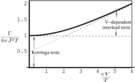
Figure 2: Voltage-dependent spin-relaxation rate, computed to leading quadratic order in the Kondo coupling constant, showing the zero field, Korringa component, and the the voltage-dependent inter-lead component. For the case chosen, $\bar{J}_{\lambda\lambda^{\prime}}=\bar{J}$ ($\lambda,\lambda^{\prime}\in\{R,L\}$).

The effect of applying a voltage to the leads can be incorporated into the self-energies by noting that a voltage is equivalent to a gauge transformation on the conduction electron fields, $c_{k\lambda\sigma}\rightarrow c_{k\lambda\sigma}e^{i\mu_{\lambda}t}$, where $\mu_{\lambda}$ is the chemical potential shift in the $\lambda=L,R$ lead. In a second-order calculation, this gauge transformation can be incorporated by making the replacement $\omega\rightarrow\omega-(\mu_{\lambda}-\mu_{\lambda^{\prime}})$ in each term of the self-energy, so that at finite voltage

$$\Sigma_{R}(\omega) = 4\sum_{\lambda,\lambda^{\prime}}(\bar{J}_{\lambda\lambda^{\prime}})^{2}\Upsilon[\omega-(\mu_{\lambda}-\mu_{\lambda^{\prime}})],$$ (34)

$$\Sigma_{K}(\omega) = -4\pi i\omega[\bar{J}_{RR}^{2}+\bar{J}_{LL}^{2}+2\bar{J}_{RL}^{2}],$$ (35)

where the voltage dependence cancels out of the second expression. Using (30) we may immediately read off the leading order expression for the voltage-dependent spin relaxation rate of a quantum dot:

$$\Gamma_{0}(V,T)=4\pi\bar{J}_{RL}^{2}\left[2\alpha T+eV\coth\left(\frac{eV}{2T}\right)\right],$$ (36)

where we have introduced $eV=\mu_{L}-\mu_{R}$ and $\alpha=(\bar{J}_{LL}^{2}+\bar{J}_{RR}^{2})/2\bar{J}_{RL}^{2}$. (See Fig. 2.) We recognize the $V=0$ limit of (36) as the Korringa relaxation rate of a single spin langreth72 . At finite $V$, the second term gives the voltage-dependent spin relaxation rate induced by the coupling between leads: this term is linear in temperature for $eV\ll T$, but linear in voltage for $eV\gg T$. An identical result for ${\bar{J}}_{\lambda\lambda^{\prime}}={\bar{J}}$ was obtained in ref. plihal01 . We can also read off the voltage-dependent fluctuation-dissipation relation (see Fig. 3),

$$h(\omega)=\frac{(1+\alpha)\omega}{\frac{1}{2}[\phi(\omega+eV)+\phi(\omega-eV)]+\alpha\phi(\omega)},$$ (37)

where $\phi(x)={x}\coth(x/2T)$, so that by (18) the static susceptibility is given by

$$\chi(V,T)=\frac{1}{4T}\frac{(1+\alpha)}{[(eV/2T)\coth(eV/2T)+\alpha]},$$ (38)

corresponding to a voltage-dependent Curie susceptibility.

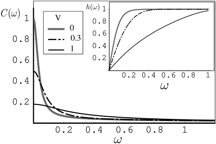
Figure 3: Voltage-dependent spin correlator $C(\omega)$ calculated for a sequence of voltages $V=0,\,0.3,\,1$ at a temperature $T=0.05$. Here $\alpha=1$ and $\bar{J}=0.2$. Inset, fluctuation dissipation function $h(\omega)$ for the same sequence of voltages.

This result confirms earlier results of Parcollet and Hooley parcollethooley , obtained by a direct calculation of the magnetization using a self-consistent expression for the Keldysh Green’s function. Parcollet and Hooley also obtain the finite field result $M(B)=\frac{1}{2}h(B,V)$, which suggests that the voltage-dependent fluctuation-dissipation theorem is independent of field at weak coupling.

Clearly, although this is beyond the scope of the current paper, the approach taken above can be extended to higher orders. An interesting question that this may help answer is whether the coherence of the Kondo effect is preserved at high voltage bias for the (physical) antiferromagnetically coupled quantum dot Kaminski:2000 ; Wen:1998 ; ColemanPH ; Roschgroup .

One of the enticing possibilities that this method offers is that of extension to more complex, multi-impurity or even lattice spin problems. The proportionality between spin and Majorana fermions can be extended to these cases, merely by introducing an independent Majorana fermion $\Phi_{j}$ for each spin site, and writing $\vec{\eta}_{j}=2\Phi_{j}\vec{S}_{j}$. The generalization of (3) to a lattice is then

$$S_{i}^{a}(t_{1})S_{j}^{b}(t_{2})=\frac{1}{2Z_{ij}}\eta^{a}_{i}(t_{1})\eta^{b}_{j}(t_{2})$$ (39)

where $Z_{ij}=2\langle\Phi_{i}\Phi_{j}\rangle$. The quantity $Z_{ij}$ is a constant of motion that acts as a type of $Z_{2}$ gauge field. Closely related identities have recently been used to solve an anisotropic Heisenberg model on a honeycomb lattice kitaev . The extension of these ideas to a Kondo lattice model, and its possible link to $Z_{2}$ gauge theories senthil may be of particular interest to future research.

We should like to thank O. Parcollet for extensive discussions related to this work. This work was supported by DOE grant DE-FG02-00ER45790 (PC, DL, WM), and the EPSRC fellowship GR/M70476 (CH). After posting this work, we discovered that Shnirman and Makhlin have independently arrived at similar conclusionsshnirman .

References

(1)A. A. Abrikosov, Physics 2, 5 (1965).
(2)J. Schwinger, Quantum Theory of Angular Momentum, edited by L. Biedenharn and H. V. Dam (Academic, New York, 1965).
(3)D. P. Arovas and A. Auerbach, Phys. Rev. B 38, 316 (1988).
(4)C. Jayaprakash, H. R. Krishnamurthy and S. Sarker, Phys. Rev. B 40, 2610 (1989).
(5)C. L. Kane, P. A. Lee, T. K. Ng, B. Chakraborty and N. Read, Phys. Rev. B 41, 2653 (1990).
(6)For concise list of early references on Majorana fermions,
see A. M. Tsvelik, “Quantum Field Theory in Condensed Matter
Physics” (Cambridge, 1995.)
(7)
H. J. Spencer and S. Doniach, Phys. Rev. Lett. 18, 23, 1967.
(8)V. R. Vieira, Phys. Rev. B23, 6043, 1981.
(9)P. Coleman, E. Miranda and A. Tsvelik, Phys. Rev. Lett. 70, 2960–2963 (1993).
(10)B. Sriram Shastry and Diptiman Sen, Phys. Rev. B 55,
2988–2994 (1997).
(11)P. Coleman, E. Miranda and A. Tsvelik, Phys. Rev. Lett. 74, 1653 (1995).
(12)For a review of Keldysh method, see J. Rammer and
H. Smith, Rev. Mod. Phys. 58, 323 (1986).
(13)D. Langreth and J. Wilkins, Phys. Rev. B 6,
3189 (1972).
(14)M. Plihal, P. Nordlander and D. Langreth, cond-mat/0108525.
(15) O. Parcollet and C. Hooley, Phys. Rev. B 66, 085315 (2002).
(16)A. Kaminski, Yu. V. Nazarov and L. I. Glazman, Phys. Rev. B 62, 8154 (2000).
(17) X.-G. Wen, LANL preprint cond-mat/9812431.
(18)P. Coleman, C. Hooley and O. Parcollet, Phys. Rev. Lett. 86, 4088 (2001).
(19)A. Rosch, J. Paaske, J. Kroha, and P. Wölfle,
Phys. Rev. Lett. 90, 076804 (2003).
(20)A. Kitaev, private communication (2002).
(21)T. Senthil and M. P. A. Fisher, J. Phys. A 34, L119-125 (2001).