COMPASS : An Instrument for Measuring the Polarization of the CMB on Intermediate Angular Scales

Abstract

COMPASS is an on-axis 2.6 meter telescope coupled to a correlation polarimeter. The entire instrument was built specifically for CMB polarization studies. Careful attention was given to receiver and optics design, stability of the pointing platform, avoidance of systematic offsets, and development of data analysis techniques. Here we describe the experiment, its strengths and weaknesses, and the various things we have learned that may benefit future efforts to measure the polarization of the CMB.

1 Instrument Design

COMPASS was designed to measure the polarization of the CMB on intermediate angular scales. Here we describe the major components of the instrument and how it performed in the field. There are essentially three major parts: the receiver, the optics system, and the pointing platform. An addendum concerning the observing site is included as well. Note that further details on any part of the experiment discussed in the paper are available [7].

1.1 Receiver Description

The polarimeter implements state-of-the-art HEMT (High-Electron Mobility Transistor) amplifiers that operate in the 26-36 GHz frequency range (Ka band). These amplifiers provide coherent amplification with a gain of $\approx 25$ dB. To reject $1/f$ noise from the detectors and atmospheric fluctuations two HEMTs are configured as an AC-biased correlation receiver. Each HEMT amplifies one of two polarizations observed through the same horn and thus the same column of atmosphere and same location on the sky at a given time. The resultant amplified signals are mixed down to 2-12 GHz, phase modulated at 1 kHz, multiplexed into three sub-bands, and further amplified along separate but identical IF amplifier chains. The signals are then multiplied together and the 1 kHz switch is demodulated. The resulting correlated signal time-averaged amplitude is proportional to one linear combination of the Stokes parameters (Q or U in the detector’s frame) as determined by the paralactic angle of the observations and the orientation of the receiver axes. A second linear combination can be obtained after a $45\mbox{${}^{\circ}$}$ rotation of the polarimeter about the horn’s optical axis thus allowing one to measure both Stokes parameters and thus obtain all information about the linear polarization. For the observations reported here no rotation was performed; solely the detector’s U polarization was measured. Depending on the observation strategy this will then map to some linear combination of Q and U Stokes parameters, and similarly “E” and “B” symmetry modes, on the celestial sphere. Details for our observations are provided in section 2.4.

The three sub-bands, in order of decreasing RF frequency, are termed J1, J2, and J3. Each of these sub-bands is demodulated with waveforms both in and out of phase with the phase-modulation signal. Thus the desired signal is obtained from each in-phase demodulation (called J1I, J2I, and J3I) in addition to a null-signal noise monitor from the out-of- phase demodulation (J1O, J2O, and J3O). Further, a power splitter prior to the multiplexing stage allows a total power detection of each linear polarization termed TP0 and TP1.

This receiver was originally coupled to a corrugated feed horn with a $7\mbox{${}^{\circ}$}$ FWHM beam for a large angular scale CMB polarization experiment known as POLAR [10]. For further details of the receiver please see Keating et. al. [11]. In order to observe smaller angular scales where a larger primordial polarization signal is expected a dielectric lens was added to the POLAR optical system and this horn+lens combination was coupled to a 2.6-meter on-axis Cassegrain telescope to form COMPASS .

1.2 Telescope Description

The COMPASS optics were designed to be as free from systematic effects as possible. Oblique reflections of light off metallic surfaces induce spurious polarization. In the case of a single angle of incidence onto a flat mirror the induced polarization is given by [16]

$$P=\big{[}\frac{\omega\mu}{2\pi\sigma}\big{]}^{(1/2)}\sin{\theta}\tan{\theta}.$$ (1)

Here $\theta$ is the angle of incidence, $\omega$ is the angular frequency of the incident light, $\mu$ us the magnetic permeability, and $\sigma$ is the DC electric conductivity. For Aluminum Alloy, 6061-T6, at microwave frequencies these numbers are typically $\mu\sim 1$ and $\sigma\sim 2.31\times 10^{17}$ Hz.

In any off-axis telescope there will be an average angle of incidence resulting in a systematic polarization for at least one Stokes parameter. To avoid this effect COMPASS implemented an on-axis Cassegrain configuration. (Note that this systematic polarization can be somewhat reduced for an off-axis observation through the use of a fold mirror or optics which satisfy the Dragone conditions, though discussion of these solutions is beyond the scope of this paper.)

Despite the great reduction in overall systematic polarization in an on-axis system it is still possible to obtain a net instrumental polarization for a given Stokes parameter (expressed in the detector coordinate system). If there is a net quadrupolar temperature distribution of the optical system that is not orthogonal to the observed polarization axes a systematic polarization will result. Such a primary mirror temperature profile is likely to arise during periods of changing thermal conditions such as sun rise and set. To understand how significant this effect could be the temperature of the COMPASS primary mirror was measured at eight locations allowing decomposition into the dipole and quadrupolar components. We induced a variety of temperature profiles using mirror-mounted heaters and measured the resulting polarized offset. The results of this test are provided in figure 1. To minimize this effect during observations the back of the mirror was insulated with conventional fiberglass insulation and “reflectix” insulation. An estimate of the maximum induced polarization signal on the timescale of one scan is given in figure 1. This allows us to set an upper limit of 0.2 $\mu K$ of induced signal from this effect during our CMB observations.

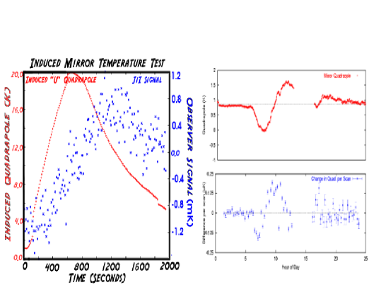
Figure 1: Effects of mirror quadrupolar temperature distribution. The left image shows the calibration data where a quadrupole temperature was applied to the mirror with heaters. The top right shows the actual quadrupole as a function of time of day, as measured by mirror mounted thermometers,on March 25, 2001, and the bottom right an estimate of the maximum induced signal given the other two plots.

Scattering or diffraction by a metal or dielectric will also induce a polarized signal [12]. In conventional on-axis systems metallic or dielectric secondary supports (often termed “struts”) necessarily obstruct the optical aperture. This will give rise not only to an overall polarization but also an increased side-lobe level. To avoid both of these effects COMPASS uses a radio-transparent expanded polystyrene (EPS) secondary support system. Finite Element Analysis (FEA) was used to design this foam support system to minimize the optical depth while providing sufficient stiffness to position and stabilize the secondary mirror with 1 mm resolution.

Many types of foam were measured for their emissivity and reflectivity at Q (36-44GHz) and W (88-102 GHZ) bands. Our final candidates were various densities of EPS. A conical shape was chosen for this support structure with the additional of metallic rings at the center and periphery of the cone to add stiffness. Neither of these rings is visible to the detector. As a trade off between maximizing the stiffness of the structure and minimizing its optical depth EPS of two pounds per cubic foot was selected.

The success of this approach was tested through beam maps of the system using a Gunn oscillator located in the mid-field for each of two configurations: support of the secondary mirror with conventional, optimized metallic struts and with the foam support. Use of this cone when compared to the conventional optimized strut configuration reduced the first sidelobe from -30 dB to -45 dB as shown in figure 2.

Figure 2: Beam maps of the COMPASS main lobe and first sidelobes using a mid-field source in two different secondary support configurations: EPS and struts. Note that the larger FWHM of the strut configuration is because the source was closer to the telescope resulting in an effectively larger beam. Note also that the first sidelobe is reduced from -30dB to -45 dB through use of the EPS support.

The secondary mirror was designed to minimize aperture blockage. The primary mirror that was acquired had a hole of 30 cm diameter in its center, thus the secondary was constructed with a 30 cm diameter. A hole was left in the center of this mirror to prevent re-illumination of the receiver and a polarized IR calibrator placed behind this hole. To reduce edge illumination of the primary the edge of the secondary mirror is designed to illuminate a surface 7 cm in from the edge of the primary thus giving a much faster than Gaussian taper to the edge illumination. This results in reducing ground pickup and spillover while still maintaining a small beam size. The illumination of the primary was measured to be less than -25dB at the edge. A one dimensional plot of the primary illumination pattern is provided in figure 3.

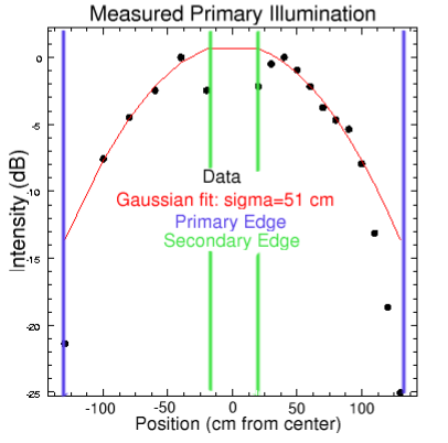
Figure 3: A map of the measured primary mirror illumination vs. distance from the center.The rapid edge taper and effect of the central hole are readily apparent at large and small radii, respectively.

In order to minimize the illumination at the edge of the secondary mirror using the existing microwave horn and dewar it was necessary to reduce the beam size from 7 degrees FWHM to 5 degrees FWHM with a lens. The additional requirement that this lens be cooled to reduce its contribution to the system temperature necessitated that the lens be mounted close to the horn and thus be approximately the same diameter as the horn. A simple meniscus phase-correcting lens was selected which resulted in -15dB secondary edge illumination. This design was based on the work by [12] and has a spherical inner surface, whose radius matches that of the radius of the horn-produced Gaussian beam, and an ellipsoidal outer surface designed to give a flat phase front at the entrance surface of the lens.

A second design that was considered was a biconvex lens. Using Gaussian optics theory [8] we can consider this lens as reimaging the beam waist of the horn. The radii were chosen to reimage the waist a distance d in front of the horn with d also the lens to beam waist distance. This provides the same far field resultant beam but would give a lower edge illumination at the secondary as shown by figure 4. Because the theory, focal point, and beam shape were better understood for the meniscus lens, however, it was selected for use. Though this resulted in a more aggressive illumination of the secondary than desired most of the excess power comes from the sky and thus was not anticipated to produce significant systematic effects. Unfortunately, systematic effects were observed and this aggressive illumination may well be the cause.

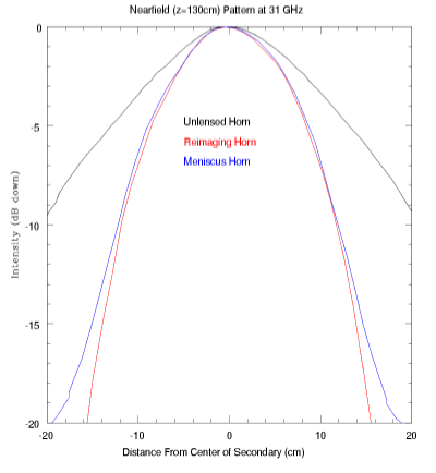
Figure 4: Comparison of the beam patterns of meniscus and bi-convex lenses at the distance of the COMPASS secondary mirror.

To further reduce COMPASS ’ sensitivity to possible systematic effects two levels of ground screens, one affixed to the telescope and the other stationary, were constructed. The screens which were mounted to the telescope were attached directly to the edge of the primary mirror. These provide an additional $>50$ dB of attenuation to signals from the ground, sun, and moon in addition to the already low sidelobe level (-60 dB) of the telescope at the location of these contaminants. Observations were conducted both with and without the outer (stationary) ground screens present. Data collected with the outer groundscreens present suffered from a larger scan synchronous signal (SSS) than data taken with them absent. It is believed that the combination of telescope spillover with the oblique scattering angle off the metallic surface of the groundscreens induced a large polarized offset. This will be discussed in more detail in section 3.2. This demonstrates that even more than exceptional care must be given to designing a CMB polarization experiment to be immune to systematic effects.

1.3 Platform Description

COMPASS is based on a standard Az-El pointing platform. The azimuth and elevation stages are separate units. The azimuth table used was a refurbished and improved version of an existing table previously designed for use with CMB observations from the South Pole. The elevation stage was designed and built for this experiment.

The table consisted of a 3/8” thick Aluminum plate reinforced with 1.75” long fins protruding from the bottom. These fins attached to a conically shaped plate which rode upon four conical roller bearings which supported the weight of the telescope. A 12” diameter roller bearing at the center connected the table to the base. The base was composed of light-weighted Aluminum beam and a 1/2” thick plate. Wheels and screw jacks were attached to this base allowing either mobility or stability. The table was, however, designed for a 1.3 m dish and its associated load and thus proved to be insufficiently stiff to support the COMPASS mirror. Several methods of improving the table were investigated. The simplest satisfactory result involved rigidly bolting the elevation base’s 3” Aluminum box beam to the table. After this modification the table deflected less than 1/16” and did not tilt (i.e. $<1^{{}^{\prime}}$) when scanning in Azimuth as per our scan strategy (see section 2.4 for details). Further, the rotation platform’s support structure was replaced with a 12” Aluminum I-beam (W12x7) triangle with a 1/2” thick Aluminum plate welded to its top. The angular deflection under 1000 ft-lbs for this base is much less than $1^{\prime}$.

The table was actuated by a stepper motor driving a harmonic drive gear reducer which rotates one of the 4 conical bearings described above. The harmonic drive has a gear reduction of 60:1 and the ratio of the radius of the bearing to that of the surface it drives yields a further reduction of 6:1 resulting in a 360:1 net gear reduction. Using our 200 step/revolution, 5 ft-lb motor allows us a single step resolution of better than 20 arc seconds and the ability to drive torques up to 1800 ft-lbs. Unfortunately the effective torque specification of this stage was limited by the friction between the bearings and the conical plate. In periods of high wind pointing control was lost and the associated data ignored. Hard stops were implemented which prevented motion of more than a few degree outside the desired scan region. One important lesson to learn from this, however, is that friction drive based systems can not apply sufficient torque to control a mid-size telescope in periods of even moderate wind and should be avoided.

The mechanical coupling of this drive system was improved by firmly bolting all members and removing backlash from the harmonic drive with shim material. The compliance and backlash were tested by projecting a 1/8” diameter laser beam mounted to the base to a wall 100 feet away. A backlash of less than 1.1’ and a compliance of 1.5’ were observed using this method which was later confirmed when performing beam maps to test the optical system. These specifications are sufficient for our 20’ beam.

The elevation axis was driven by a ball-screw linear actuator of 60” length when extended with 26” of stroke to allow observations at any elevation. The actuator was driven by a 40:1 worm gear which was coupled to a reducer and stepper motor. The pitch of the worm gear assures that the actuator cannot be driven backward, the ball-screw grants low backlash and compliance, and the stepper motor and reducer are chosen to provide sufficient resolution and speed.

The position of each axis was read out by a Gurly 16 bit encoder giving a resolution of 20 arc seconds. The mounting locations of the encoders were chosen so that they supported no torque thus assuring accurate readout of the coordinates. Data acquisition of all radiometer, pointing, and “house keeping” data (such as thermometry) as well as telescope control were performed with a Pentium class laptop computer and 48 channel 16-bit ADC purchased from Iotech.

Our campaign took place at the University of Wisconsin’s Astronomy observatory in Pine Bluff, Wisconsin (89.685 West longitude, 43.078 north latitude) 100 meters from the platform used for the POLAR observations. As a ground-based experiment located within twenty miles of the UW main campus COMPASS had the advantage of being deployed and staffed relatively easily. Though some sensitivity and observing time is sacrificed because of poor atmospheric conditions, the advantage of being able to repair and adjust the telescope during the course of the observations was invaluable. The site chosen used a 60’x30’ tensioned fabric building with a wheeled, aluminum frame to house the telescope [1]. This building was rolled 20 m to the South of the telescope on tracks for observations and rolled over the telescope for suitable shelter during periods of foul weather. By moving the building rather than the telescope we were assured of the stability of the telescope and its celestial alignment.

2 Instrument Characterization

Once deployment began in mid-January of 2001 a number of crucial tests needed to be performed to understand the performance, and results, of the experiment. These include the calibration, beam characterization, and pointing of the telescope. We also include here a discussion of our scan strategy.

2.1 Calibration

There are three bright objects visible in the northern hemisphere with sizable average polarization and angular size of less than several arc-minutes. These are Tau A (The Crab Nebula), Cas A, and Cyg A with polarized signals at 30 GHz of $\sim 23.5$ [9], 1.94 [13], and 1.1 Jy [14], respectively. With our $19.6^{{}^{\prime}}$ beam and the noise in our correlator channels, these correspond to a signal to noise ratio in one second of observation of $\sim$ 20, 2, and 1. Clearly Tau A is our primary source candidate for calibration.

Factors	J3I	J2I	J1I
Ant. Temp. (mK)	$11.8\pm 2.5$	$9.6\pm 2.1$	$7.7\pm 1.7$
inv. Tele. eff	2.68
atm.	0.988
RJ, CMB	1.020	1.024	1.029
cosmo/astro	0.5
decay	0.947
Signal (mV)	$12.4\pm 0.37$	$5.15\pm 0.14$	$3.59\pm 0.16$
Gain (K/V)	$1.2\pm 0.4$	$2.4\pm 0.9$	$2.8\pm 1.2$

Table 1: Provided are the various calibrations for our 3 correlator channels and two total power channels derived from observations of the Crab Nebula. “atm.” indicates corrections for atmospheric absorption, “RJ, CMB” for the conversion from Raleigh-Jeans to thermodynamic temperature, “cosmo/astro” is described in the text, and “decay” for the decay of source brightness since the measurements of [9].

The present day flux for Tau A and our expected signal are calculated using the polarized observations of Johnston and Hobbs [9] adjusted for the observed decay rate of Allers [3], and spectral index of Baar [5]. Johnston and Hobbs measured a flux of $313\pm 50$ Jy at a frequency of 31.4 GHz with 8.1% polarization at a polarization angle of $158^{o}$. The flux of Tau A is known to be decreasing with time at a rate of $0.167\%\pm 0.015\%/$year [3]. The flux density spectral index is measured to be $\alpha=-0.299\pm 0.009$ [5] so the polarized antenna temperature is taken to be $P_{Jx}\propto(\nu_{GHz}/31.4)^{-2.299}$. Several corrections are performed as summarized in table 1. Most notable is a change in convention between cosmologists and astronomers and is obtained by dividing by two [15]. This later correction is driven by the Rayleigh-Jeans law where we take:

$$S=2\frac{k_{B}T}{\lambda^{2}}$$ (2)

The factor of 2 arises because there is radiation in both polarization states. Thus if one is calculating the total flux of a source it is consistent to define:

$$S=\frac{k_{B}}{\lambda^{2}}(T_{x}+T_{y})$$ (3)

where $x$ and $y$ are the two measured polarization states. From a radio astronomer’s point of view one would report Tx+Ty allowing direct conversion to flux units. In order for the CMB cosmologist to maintain consistency with equation 3 therefore would dictate that one define $2T=T_{x}+T_{y}$, or similarly:

$$T_{I}=\frac{(T_{x}+T_{y})}{2},$$ (4)

and therefore also

$$T_{Q}=\frac{(T_{x}-T_{y})}{2}.$$ (5)

We have added the subscript $I$ and $Q$ to denote the total intensity and “Q” polarization temperatures respectively. Our definition is in agreement with existing CMB polarization experiments and is consistent with CMBFAST [2] where one requires that $T_{I}$ and $T_{Q}$ have the same numerical prefactor. The expected signal and all necessary corrections as a function of channel is shown in table 1. We are currently finalizing the calibration by considering Tau A observations by other observers.

2.2 Pointing

We initially pointed the telescope by co-aligning an optical telescope mounted on the primary mirror with the cm-wave beam pattern using a 31 GHz Gunn oscillator mounted on a radio tower 1.9 km West-by-Southwest from the telescope (see section 2.3 for details). The source on the radio tower was quite easily visible with the optic selected. Because of the proximity of our observing region to the NCP several optical observations of Polaris and a number of nearby stars were made. These Polaris observations were then used to define our absolute azimuth and elevation offset and thus to define our observing region. Unfortunately, misalignment of the optical telescope resulted in an azimuth and elevation pointing error of $+0.458\pm 0.027$ and $-0.107\pm 0.023$ degrees respectively.

This pointing offset was discovered through observations of the supernova remnant Cas A. Cas A is circumpolar from our observing location, fairly close to our observing region, and quite bright in intensity, making it useful as a pointing tool. Three observations were made throughout the season as outlined in table 2. Through linear fits the elevation is seen to drift at $-1.43\pm 2.3$ arcminutes in Elevation and $10.1\pm 6.9$ arc minutes in Azimuth per month; There is no compelling statistically significant evidence for drifts in the pointing over the given 52 day period. Thus, a fixed pointing offset was used for all files in the analysis. This also gives us confidence that EPS secondary supports are indeed stable enough, and transparent enough, to be used in precision observations.

Day	Obs.	Az	error	El	error
62	4	17.4	6.6	-5.4	4.2
109	2	40.8	1.8	-10.2	2.4
114	6	29.4	4.3	-6.0	1.8
ave		37.8	1.6	-7.3	1.4
RMS		12.6		2.1
wRMS		5.3		1.8

Table 2: Successful observations of Cas A were made on the days specified by the day number in the first column. Obs. gives the number of full, independent rasters performed at that time. The azimuth and elevation offsets and errors are given in the remaining columns. ave provides the weighted average, and thus the offsets used in analysis, RMS the scatter of the individual measurements, and wRMS the scatter weighted by the uncertainty of each measurement.

2.3 Beam Determination

Raster maps of the above-mentioned “tower source” were made by maintaining constant elevation while scanning in azimuth with elevation changes performed at turn-around points. This “tower source” was a 31-GHz Gunn oscillator mounted on a radio tower 1.9 km West-by-Southwest of the telescope. This was essentially in the far field of the telescope requiring only a 0.1’ correction to the beamwidth at infinity. The source was mounted on the tower and could be turned on and off with a very long extension cord; thus allowing it to be bright enough for our use as a tool but not worrisome as a signal contaminant during observations. This Gunn oscillator was mounted to a scalar feed horn in a sealed PVC tube with foam endcaps. Thus it was sealed against weather and quite easily visible with the optical telescope which was mounted on the primary mirror and thus coaligned with the optical beam.

The FWHM obtained by fits of a Gaussian to the elevation and azimuth directions for two separate days of tower source observations are 19.2 $\pm$ 0.4 and 20.3 $\pm$ 0.5 arcminutes respectively. These beam maps are confirmed by scans of Tau A. A fit of these maps with Tau A deconvolved yield a FWHM for each polarization channel and each direction ( elevation and cross-elevation) as provided in table 3.Note that the analysis of the Tau A data requires time series filtering which may induce a larger beam size. These numbers are further confirmed by observations of Venus which is a point source in our beam and yields beams of the two total power channels of $18.5^{{}^{\prime}}\pm 1.0^{{}^{\prime}}$ and $19.6^{{}^{\prime}}\pm 0.8^{{}^{\prime}}$. In our likelihood analysis we make the approximation that the beam is axially symmetric with FWHM $20.0^{{}^{\prime}}$ an approximation which affects our result by $\leq$ 5%.

Channel	Cross-Az	elevation
J1I (32-35)	$21.5\pm 0.9$	$20.2\pm 0.9$
J2I (29-32)	$22.0\pm 0.7$	$21.5\pm 0.9$
J3I (25-29)	$23.2\pm 0.7$	$23.2\pm 0.9$

Table 3: FWHM of the beam on the sky of each sub-band derived from observations of Tau A, in arcminutes. All are biased somewhat high because of the data processing performed

2.4 Observing Strategy

Our observing strategy was designed to optimize the probability of detecting a signal under current well-motivated theories while still allowing for systematic checks and tests. We attempted to observe a circular “disk” region centered on the North Celestial Pole (NCP) by maintaining a constant elevation and scanning the telescope in azimuth. During constant-elevation scans the thermal load from the atmosphere remains constant and reduces both gain fluctuations of the receiver and intensity-polarization coupling in the polarimeter that could cause systematic effects. Our full scan period was varied between 10 and 20 seconds to reject longer term atmospheric fluctuations while maintaining stable and reliable telescope performance.

As the sky rotates this scanned line is transformed into a cap centered on the NCP as demonstrated in figure 5. Further, because of the sky rotation, each half sidereal day the same region of sky is observed and allows the use of difference maps as a robust test of systematic errors. Initially this “cap” was one degree in diameter in order to allow deep integration on a small patch of sky to search for systematic effects. Half way through the season this diameter was increased to 1.8 degrees to allow a trade-off between sample variance and noise-induced errors. As mentioned above there was a small pointing offset so our actual scan strategy was not the one we intended. This resulted in a loss of symmetry and thus some systematic tests but acceptable noise properties. Given the relative sizes of our beam, scan region, and pointing offset from the NCP our telescope is sensitive to both “E” and “B” symmetry modes at roughly the same level.

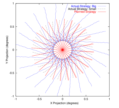
Figure 5: COMPASS scan strategy in rectangular projection about the NCP. The axis are real degrees on the sky with the positive x-axis corresponding to a Right Ascension of 0. It is clear how constant Elevation Azimuth scans are transformed into a two dimensional map through sky rotation.

One further benefit of this scan strategy is that it simplifies the process of encoding the time stream data into a map which displays well the SSS while still allowing for reasonable cross-linking, sampling of a variety of paralactic angles and excellent systematic tests. As mentioned below, a one dimensional to two dimensional map comparison allows simple identification of SSS. If we plot out data in a coordinate system defined as Azimuth and Right Ascension it becomes quite easy to combine the data across many days and project out the modes that correspond to SSS (see section 4).

Finally two configurations of the ground screens were implemented; one utilizing the two layers mentioned above and one with only the inner, co-moving ground screen. These two options, combined with the two scan amplitudes mentioned above, result in a total of four sub-seasons of data termed SIGS, SOGS, BIGS and BOGS to specify whether the (S)mall or (B)ig scan was used and weather the (O)uter or only (I)nner ground screens were in place. Analysis was performed on each channel in each sub-season as well as combinations of channels within a sub-season, combinations of sub-seasons for a given channel, and all acceptable data.

3 Data Characterization

Here we give a preliminary glance at the data emphasizing our selection process, data characterization, statistical checks, and analysis pipeline.

3.1 Data Selection

There were a total of 1776 hours available during our observing season which was defined as the months of March, April, and half of May of 2001. Of these 409 were sufficiently good weather to operate the experiment. 74 hours were ignored because heavy winds disrupted the Azimuth pointing and control and 28 hours were removed because of equipment failures. This leaves a total of 309 hours of usable data observing the target region. Further cuts are made to select periods of stable observing conditions.

The data are divided into files of 15 minutes in length. For each file six statistics are generated: three noise-based statistics (white noise level, 1/f knee, and $\zeta$ [10]); two cross correlations (between two correlator channels and between a correlator and total power channel); and a linear drift of the time stream. The 1/f knee and $\zeta$ statistics proved to be most sensitive to periods of light cloudiness or haziness. The cross correlations were most useful in identifying more rapid contaminating events such as discrete clouds, birds, or planes interfering with the observations. Finally the linear drift was used to identify dew formation on the foam cone.

This dew formation was the one drawback of the foam secondary support. This problem is conceivably circumventable with the use of IR lamps, fans, or some similar technology. Fortunately it was quite easy to identify periods of excessive dew formation as the correlator outputs would drift up as the dew formed and down as it evaporated. Once this data was cut using the linear fit to the time stream there is no evidence that such periods further corrupt the data.

A histogram of each statistic is formed and unions and intersections are made of files passing sets of cuts at the 3-$\sigma$ level. Our results were not overly sensitive to which sets were selected. The results reported here use the two cross-correlation criteria for they retained the most data while still passing all null-tests performed (see below). A pictorial summary of the cuts considered is shown in figure 6

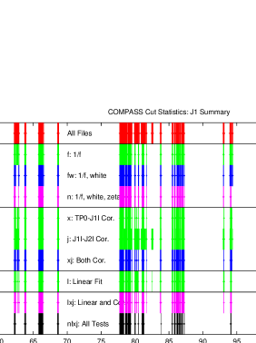
Figure 6: COMPASS data selection summary for one channel (J1). Time proceeds along the x axis with each vertical line representing a 15 minute file that passed the indicated cut. Green lines indicate that only a single cut was performed while blue indicate multiple cuts were used. Magenta and black indicate cuts that were used in actual full analysis runs.

Each file is also passed through a despiking procedure. Regions with excessive slopes, second derivatives, or values greater than 5 standard deviations from the mean are flagged, cut, and filled with white noise as estimated by the remainder of that file. This procedure removes between 0.1 % and 32% of the data from any give sub-season. The 32% was an anomaly; it occurred only for one channel, J3, during the first sub-season where a damaged preamplifier gave rise to excessive spikes in the data intermittently. This was fixed once the cause was identified. After all selection procedures the number of hours kept were 144, 123, and 164 for J1, J2, and J3 respectively.

3.2 Scan Synchronous Signal

One common systematic error in scanning style experiments is the presence of non-celestial signal that correlates highly with the scan, termed here “Scan Synchronous Signal” (SSS). In COMPASS such SSS was observed and was related to a polarized offset induced by oblique reflection from the stationary ground screen or spillover to the ground. In all sub-seasons a variable offset and linear term (when plotted against Azimuth) are observed and removed. In the larger scan with the stationary ground screen present a quadratic signal is detected and removed as well. Once these removals have been performed the residual is consistent with Gaussian noise.

Detection of the SSS is performed easily by comparing maps made by binning the data in the (one) scan dimension (i.e. Azimuth for COMPASS ) to those made by binning in two (i.e. Azimuth and Right Ascension). If one has SSS contamination the relationship between the reduced chi-squared of the one dimensional map to that of the two dimensional map is given by

$$\chi^{2}_{1D}=1+N_{\text{bin}}\times(\chi^{2}_{2D}-1),$$ (6)

where $N_{\text{bin}}$ is the number of bins in the dimension that is not present in the one dimensional map, and $\chi$ refers to reduced chi squared for each map. As shown for a typical channel in table 4 there is no evidence for SSS remaining in any of the sub seasons after removal of a first order polynomial other than the BOGS configuration.

	Two-D maps		One-D maps
Sub-Season	DOF’s	$\chi^{2}$	DOF’s	$\chi^{2}$
SIGS	244	1.00	13	0.76
SOGS	232	1.09	13	0.45
BIGS	182	1.08	18	0.93
BOGS	217	1.24	19	3.96

Table 4: The Chi-squared tests for RA-Az and RA-Az binned maps for all sub-seasons for channel J1I. Note that all are consistent with no signal except BOGS which does show clear signs of unremoved Scan Synchronous Signal.

In order to be insensitive to this contaminant we remove a polynomial fit (second order for BOGS data, first for all others) from each Azimuth scan (roughly ten seconds of data) for each channel. When producing the noise covariance and associated likelihood we then must, and do, apply the constraint that this mode be ignored (see section 4).

3.3 Map Making

In order to estimate a power spectrum from our data it is necessary to produce a map of our results. By the term “map” here we mean a pixelized representation of the data which contains information on the spatial location, most likely data value and (non-diagonal) noise correlation matrix. The nature of polarized observations requires different mapping procedures than a simple intensity map. Traditionally either a map of polarized intensity and orientation or a map of the Q and U Stokes parameters are provided. As COMPASS observed at fixed elevation the polarization direction information is unambiguously encoded in the Right Ascension and Azimuth.

In investigating how to produce a map of this data we discovered that using a variety of maps is a very useful tool for data visualization and discovery and removal of systematic effects. We map initially each data file in Azimuth coordinates as the sky rotation on this time scale is sufficiently small that a single bin of RA is needed. This intermediate product is quite elegant in that it allows large data compression without information loss, facilitated the process of encoding the constraint matrices, and proves flexible for producing a variety of other maps for systematic tests.

One useful map format in which to display the data is RA-Az coordinates. This facilitates identification of systematic effects and spurious (or real) signals. A second map format is a three dimensional map of RA, dec, and paralactic angle. This second map, though sparsely populated, retains the polarization information of our observations and is used in power spectrum estimation, though it is less intuitive to display and interpret. Maps of the first style are provided in figure 7.

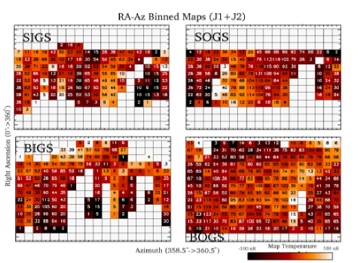
Figure 7: Maps plotted in Right Ascension and azimuth coordinates. Shown are maps for all 4 sub-seasons of the data for J1I and J2I coadded. Color indicates intensity of the signal per pixel while the number written over that pixel is the number of Az binned files that contribute to the value.

4 Data Analysis

As mentioned above, each file has an Az “map” composed of a data vector, $\vec{d_{i}}$, noise covariance matrix ($C_{n,i}$), “constraint matrix” ($C_{c,i}$), and pointing matrix as per the formalism of Bond, Jaffe, and Knox [4]. The noise covariance matrix is estimated from the timestream data. The off diagonal elements of this matrix were shown to be much less than $10^{-6}$ the amplitude of the on diagonal elements and are therefore ignored. This is because the scan rate is much slower than the anti-aliasing filter knee. This indicates that we are not making optimal use of our frequency bandwidth, but given the stability of the correlation receiver such optimization was unnecessary.

The constraint matrix encodes the SSS removal process and projects the removed modes out of the map by adding noise of amplitude $10^{8}$ that of the noisiest on-diagonal element (units of $\mu K^{2}$) to the contaminated modes. These contaminated modes are constructed for each file’s Az-map and for each order of the fit removed by forming a constraint vector and taking its outer product. As an example, consider a three element map from which we wish to remove a constant and a slope. The constraint vectors are:

$$\begin{pmatrix}1\\ 1\\ 1\\ \end{pmatrix}\text{and}\begin{pmatrix}1\\ 0\\ -1\\ \end{pmatrix}$$ (7)

with the corresponding constraint matrices:

$$\begin{pmatrix}1&1&1\\ 1&1&1\\ 1&1&1\\ \end{pmatrix}\text{and}\begin{pmatrix}1&0&-1\\ 0&0&0\\ -1&0&1\\ \end{pmatrix}$$ (8)

These constraint templates are then multiplied by the indicated (large!) noise and added to the noise covariance matrix of each file Az map. These $i$ sub-maps are then added together in RA-Az-parallactic angle space and a resultant generalized covariance matrix, $C_{N}$, and map of the data, $D$, formed as

$$C_{N,i} = C_{n,i}+C_{c,i},$$

$$C_{N}^{-1} = \sum_{i}^{M}C_{N,i}^{-1},$$ (9)

$$\vec{D} = C_{N}\left[\sum_{i}^{M}\vec{d_{i}}C_{N,i}^{-1}.\right]$$

The RA-dec-PA angle map was chosen for it eliminates pixelization effects for our beamsize and provides the most uniform pixel noise of the methods considered.

As a side note we studied the effect of removing these polynomials in this way from the data. Subtraction of a constant term resulted in weakening of our result (i.e. increasing the uncertainty of the likelihood or 2-$\sigma$ limit) by 25%. Removing a DC level and a slope weakened it by 50%! In retrospect this could have been simulated prior to the decision on our scan strategy. Our scan strategy was designed to give nearly equal noise per pixel on a number of pixels that minimized the error resulting from the combination of sample variance and statistical errors. It would have been more powerful to optimize our observing strategy to obtain the greatest number of signal-to-noise eigenmodes with eigenvalues $\approx$ 1. This analysis could have been executed including the effects of possible systematic effects.

Once these maps were obtained we proceeded to calculate a likelihood. A flat band power model of E-mode polarization appodized by our $20.0^{{}^{\prime}}$ beam was used to generate the theory covariance matrix, $C_{T}(E)$, though use of a concordance model polarization spectrum did not significantly change our results. The likelihood of the amplitude of this flat band power is calculated using the signal to noise eigenmode method as described in [4]. To reduce the time to compute the likelihood curve only modes with an eigenvaue more than $10^{-8}$ that of the most well measured mode are retained. It is worth noting that no eigenmode has an eigenvalue greater than 1. We build the total covariance matrix $C(E)=C_{T}(E)+C_{N}$ and compute the likelihood as given by

$$L(\vec{D}|C(E))=\frac{1}{(2\pi)^{N/2}}\frac{e^{-\frac{1}{2}\vec{d}^{T}C(E)^{-1}\vec{d}}}{\left|C(E)\right|^{1/2}}.$$ (10)

This likelihood is calculated on a grid spaced uniformly in units of $\mu K^{2}$ to avoid over weighting large values of the fit parameter and is allowed to take values of negative power to test the correctness of the noise covariance matrix. Note that in a low signal to noise experiment these steps, as well as computing the actual likelihood curve rather than an estimator, are crucial. When excessively negative values of power are considered one is considering unphysical solutions and the covariance matrix will no longer be positive definite. If the matrix becomes non-positive definite at some (negative) value of power that value is given a Likelihood of zero.

Software used to estimate the power spectrum was extensively tested using dozens of simulated maps generated from a known power spectrum by an independent piece of software. Each map was given hundreds of noise realizations and the statistical properties of the results studied extensively. The time stream analysis, map making, and likelihood codes were all tested independently and as a unified pipeline. Maps with no signal as well as those with a signal of a known spectrum and a variety of amplitudes were considered. After much effort the software passed all these tests. It should be noted that in this testing process we were reminded that, especially in the low signal to noise range, a likelihood estimator is a biased estimator. Our tests required a calculation of the full likelihood curve rather than the peak and curvature to obtain the correct statistical results.

The likelihood described above is performed for each sub season, for the union of all sub-seasons where a slope was removed, and for the union of all data. Similarly our analysis is performed for each frequency channel independently and for the union of all channels. As of the writing of this article the analysis is in the final stages of checking the calibration; a full discussion of the results will be presented [6].

5 Conclusion

COMPASS was a first generation, scanning style CMB polarization experiment. While only setting an upper limit COMPASS has a number of valuable lessons to teach us, or at least of which to remind us.

First in building a mount avoid the use of friction based drive systems. Less obviously, and quite triumphantly, COMPASS demonstrated that the use of a Styrofoam secondary support in an on axis configuration is sufficiently strong, stable and reliable. One must be prepared, however, to deal with dew condensation or other possible effects of weather.

In terms of experimental design we have also had emphasized two valuable points. First, one must be particularly careful about preventing, testing for, and removing, systematic effects. The more complicated nature and smaller signal of polarized observations makes this even more demanding. This leads to the second point that in designing a scan strategy one should be sure that one couples the mapping strategy well to the desired signal. This is to say that the eigenmodes measured by the experiment should be those expected to have large signal. Further one should be sure that the probable systematic effects have eigenmodes as close to orthogonal to the signal as possible. The naive approximation of studying the noise per pixel is not sufficient.

Finally, in analyzing the data two valuable insights were discovered. The use of displaying the data in a variety of map formats is tremendous, especially in that it allows the identification and removal of systematic effects. Also, one must be sure that an actual likelihood curve, rather than a likelihood estimator, is calculated if the expected signal to noise of the experiment is not much greater than one.

6 Acknowledgments

We thank John Carlstrom for loaning us the required HEMT amplifiers. This research was supported by NSF grant AST-9802851.

References

- [1] Big Top Manufacturing 3255 N. US 19 Perry, Florida 32347 1-800-277-8677 http://www.bigtopshelters.com.
- [2] Personal Communication with Uros Seljak.
- [3] H. D. Aller and S. P. Reynolds. The decrease with time of the radio flux of the Crab Nebula, June 1985.
- [4] J. R. Bond, A. H. Jaffe, and L. Knox. Estimating the power spectrum of the cosmic microwave background. Physical Review D, 57:2117–2137, February 1998.
- [5] Baar’s et. al. Astronomy and Astrophysics, 61(99), 1977.
- [6] Farese et. al. In preperation.
- [7] Philip C. Farese. Polarization of the Cosmic Fireball. PhD dissertation, University of California, Santa Barbara, 2003.
- [8] Paul F. Goldsmith. Quasioptcal Systems. IEEE Press, 1998.
- [9] R. W. Hobbs and K. J. Johnston. Polarized Brightness Distribution of Taurus A and Orion A at 9.55-mm Wavelength. Bulletin of the American Astronomical Society, 1:244–+, June 1969.
- [10] B. G. Keating, C. W. O’Dell, A. de Oliveira-Costa, S. Klawikowski, N. Stebor, L. Piccirillo, M. Tegmark, and P. T. Timbie. A Limit on the Large Angular Scale Polarization of the Cosmic Microwave Background. The Astrophysical Journal Letters, 560:L1–LL4, October 2001.
- [11] B. G. Keating, C. W. O’Dell, J. O. Gundersen, L. Piccirillo, N. C. Stebor, and P. T. Timbie. An Instrument for Investigating the Large Angular Scale Polarization of the Cosmic Microwave Background. The Astrophysical Journal Supplement, 144:1–20, January 2003.
- [12] Per-Simon Kildal, Erik Olsen, and Jon Anders. Losses sidelobes, and cross polarization caused by feed-support struts in reflector antennas: Design curves. IEEE Transactions on Antennas and Propagation, 36(2), 1988.
- [13] Brian S. Mason, Leitch Erik M., Stephen T. Myers, John K. Cartwright, and A.C.S. Readhead. An absolute flux density measurement of the supernova remnant of cassiopeia a at 32 ghz. The Astrophysical Journal, 118:2908.
- [14] S. J. Melhuish, S. Dicker, R. D. Davies, C. M. Guti rrez, R. A. Watson, R. J. Davis, Hoyland R., and R. Rebolo. A 33-ghz interferometer for cosmic microwave background observations on tenerife. Montly Notices of the Royal Astronomical Society, 305:399, May 1999.
- [15] Christopher W. O’Dell, Brian G. Keating, Angelica de Oliveira-Costa, Max Tegmark, and Peter T. Timbie. Cmb polarization at large angular scales: Data analysis of the polar experiment. preprint astro-ph/0212425.
- [16] T. Renbarger, J. L. Dotson, and G. Novak. Measurements of Submillimeter Polarization Induced by Oblique Reflection from Aluminum Alloy. Applied Optics, 37:6643–6647, October 1998.