Nonextensivity of the cyclic Lattice Lotka Volterra model

Abstract

We numerically show that the Lattice Lotka-Volterra model, when realized on a square lattice support, gives rise to a finite production, per unit time, of the nonextensive entropy $S_{q}=\frac{1-\sum_{i}p_{i}^{q}}{q-1}$ $(S_{1}=-\sum_{i}p_{i}\ln p_{i})$. This finiteness only occurs for $q=0.5$ for the $d=2$ growth mode (growing droplet), and for $q=0$ for the $d=1$ one (growing stripe). This strong evidence of nonextensivity is consistent with the spontaneous emergence of local domains of identical particles with fractal boundaries and competing interactions. Such direct evidence is for the first time exhibited for a many-body system which, at the mean field level, is conservative.

Keywords: Lattice-Lotka-Volterra model, Fractals, Reaction limited processes, Nonextensivity.

Pacs Numbers: 5.40.-a, 05.10.Ln, 05.65.+b, 82.40.Np

Many natural and artificial systems are known today to be hardly, or not at all, tractable within Boltzmann-Gibbs statistical mechanics, hence the usual thermodynamics. Such is the case of systems which include long-range interactions or long-range microscopic (or mesoscopic) memory, or other sources of (multi)fractality. Phenomena where many spatial and/or temporal scales are involved typically exhibit power laws. The celebrated Boltzmann-Gibbs (BG) entropy $S_{BG}=-\sum_{i}p_{i}\ln p_{i}$ appears to be inadequate for handling the thermostatistics associated with such situations. This is due to the fact that the corresponding stationary states do not emerge through ergodic dynamics. An ubiquitous class of the above anomalous systems have nonlinear dynamics which generate weak chaos, in the sense that the sensitivity to the initial conditions is less-than-exponential in time. Such situations quite naturally accomodate with an entropy which generalizes the BG one, namely

$$S_{q}=\frac{1-\sum_{i}p_{i}^{q}}{q-1}\;\;\;(q\in{\cal R};S_{1}=S_{BG}).$$ (1)

For independent systems $A$ and $B$ (i.e., such that $p_{ij}^{A+B}=p_{i}^{A}\,p_{j}^{B}$), this entropy satisfies $S_{q}(A+B)=S_{q}(A)+S_{q}(B)+(1-q)S_{q}(A)S_{q}(B)$. It is due to this property of nonextensivity that the thermostatistical formalism based on Eq. (1) is usually referred to as nonextensive statistical mechanics [1] (see [2] for recent reviews). This theory has received many applications in areas such as self-gravitating polytropes [3], electron-positron annihilation [4], turbulence [5], motion of Hydra viridissima [6], anomalous diffusion [7, 8], classical [9] and quantum [10] chaos, long-range-interacting many-body Hamiltonians [11], option pricing [12], particular biological processes involving a large number of degrees of freedom [13, 14], among others.

The lattice Lotka-Volterra (LLV) model [15] is known to well mimic simple chemical reactions, predator-prey systems, and other biological and echological phenomena. It has recently been studied with cyclic interactions amongst three species, as a modification to the original Lotka-Volterra model[16]. The LLV has exhibited spatial clustering and fractality, even when implemented on low dimensional lattices [17]. Since fractality is a distinct sign of nonextensivity, it is natural to pose the question whether the LLV model is indeed consistent with the nonextensive premises. The aim of the present paper is to verify that this model exhibits a strong and direct evidence of having $q\neq 1$. In particular we study the LLV model with various initial conditions, namely at a) the domain formation mode, b) the nucleus (or droplet) growth mode, c) the stripe growth mode and d) the roughening mode. Modes (b) and (c) enable, as we shall see, the direct calculation of $q$. Several analytical or numerical calculations of $q$ exist already in the literature, but this is the first time such evidence is directly provided, through the time evolution of $S_{q}$ itself, on a many-body system which is conservative at the Mean Field (MF) level.

The LLV model is a minimal complexity model, with MF conservative dynamics which can be directly implemented on lattice and involves only two reactive species $X_{1}$ and $X_{2}$ (adsorbed on a lattice support) and the empty sites of the support $S$. All reactive steps are bimolecular and the reaction occurs via hard core interactions. Schematically, the LLV model has the following form[15]:

$$X_{1}\,+\,X_{2}\quad \mathop{\rightarrow}^{k_{s}}\quad 2X_{2}$$ (3)

$$X_{2}\,+\,S\quad \mathop{\rightarrow}^{k_{1}}\quad 2S$$ (4)

$$S\,+\,X_{1}\quad \mathop{\rightarrow}^{k_{2}}\quad 2X_{1}$$ (5)

In particular, a particle $X_{1}$ adsorbed on a lattice site changes its state into $X_{2}$ when it is found in the neighborhood of another $X_{2}$ particle. This step (2a) is an autocatalytic reactive step. A particle $X_{2}$ desorbs leaving an empty site $S$, if in the neighborhood another empty site $S$ is found. This step (2b) is a cooperative desorption step. Finally, a particle $X_{1}$ can be adsorbed on an empty lattice site $S$ if in the neighborhood another $X_{1}$ particle is found. This step (2c) is a cooperative adsorption step.

We now recall briefly some of the mean field (MF) and lattice properties of the LLV, which have been studied in detail in previous works[15, 17].

In the MF approximation the LLV model, Eqs. (1), can be described via the kinetic, rate equations:

$${dx_{1}\over dt} = x_{1}(-k_{s}x_{2}+k_{2}s)$$ (4)

$${dx_{2}\over dt} = x_{2}(k_{s}x_{1}-k_{1}s)$$ (5)

$${ds\over dt} = s(-k_{2}x_{1}+k_{1}x_{2})$$ (6)

where $x_{1}$, $x_{2}$ and $s$ correspond to the mean coverage of the lattice with particles $X_{1}$, $X_{2}$ and empty sites $S$ respectively. In Eqs. (3), the mean coverages satisfy identically the conservation condition $x_{1}+x_{2}+s=C$, where $C$ is a constant which can be chosen equal to unity, corresponding to interpreting $x_{1}$, $x_{2}$ and $s$ as fractions of the overall lattice respectively occupied by $X_{1}$ particles, $X_{2}$ particles or being empty. Using $C=1$ it is possible to eliminate one of the three variables, say $s=1-x_{1}-x_{2}$, and, to reduce system (3) to two equations. This reduced system admits four steady state solutions, three of which are trivial, and one non-trivial[15]:

$$x_{1s} = 0,\,x_{2s}=0\quad(\rm{empty\,lattice})$$ (5)

$$x_{1s} = 1,\,x_{2s}=0\quad(\rm{lattice\,poisoned\,by\,}X_{1})$$ (6)

$$x_{1s} = 0,\,x_{2s}=1\quad(\rm{lattice\,poisoned\,by\,}X_{2})$$ (7)

$$x_{1s} = {k_{1}\over{k_{1}+k_{2}+k_{s}}},\,x_{2s}={k_{2}\over{k_{1}+k_{2}+k_{s}}}$$ (8)

A linear stability analysis shows that the trivial states are saddle points while the nontrivial one is a center compatible with an additional constant of motion $C^{\prime}=x_{1}^{k_{1}}x_{2}^{k_{2}}(1-x_{1}-x_{2})^{k_{s}}$[18] at the MF level. Fig. 1a depicts the temporal evolution of the system for typical values for $(k_{1},k_{2},k_{s})$ and initial conditions. The black solid line represents the concentration of $X_{1}$ and the dashed line the concentration of $X_{2}$. The motion is periodic but non-harmonic. The amplitude of the periodic motion, for given parameter values, depends solely on the initial conditions[15, 17]. At this level of description the system size does not enter into the calculations since the MF approximation involves only average concentrations.

To mesoscopically describe the system on a lattice, many details enter: lattice size and geometry, number of nearest neighbors (coordination number), interaction range, etc. To realize the square lattice LLV we adopt a typical Monte Carlo (MC) algorithm (details in [15, 17]), namely (1) At every microscopic step one lattice site is randomly chosen; (2) One of the nearest neighbors is also selected randomly; (3) If the original chosen site is $X_{1}$ ($X_{2}$) and the selected neighbor is $X_{2}$ ($S$) then the chosen site changes to $X_{2}$ ($S$) with probability $k_{s}$ ($k_{1}$); If the original chosen site is $S$ and the selected neighbor is $X_{1}$ then the chosen site changes to $X_{1}$ with probability $k_{2}$; Otherwise the system remains as it is; (4) Return to step 1.

In the MC procedure the unit of time is chosen as $1/N$, where $N$ is the total number of lattice sites (occupied and empty). For example, for square lattice, $N=L^{2}$, where $L$ is the linear size of the lattice. With this choice of micro-time, in one MC step all lattice sites are, on the average, scanned once. In Fig. 1b typical behavior of the temporal evolution of the MC concentrations is shown. In particular, the concentrations of $X_{1}$ is depicted on the full lattice of size $L\times L=2^{8}\times 2^{8}$ (solid line) and on a sublattice of size $l\times l=2^{5}\times 2^{5}$ (dotted line). Periodic boundary conditions are used in all simulations. It is clear that while on the sublattice the concentrations show oscillatory behavior with added noise, on the entire lattice the oscillations shrink. Fig. 2a gives the typical evolution of a system starting from random initial conditions (Fig. 2a (t=0 MC)). As time increases the system develops local domains and each domain behaves as a local oscillator with specific characteristic frequency. Because the various domains have different phases, globally, no oscillation are observed, in contrast with the MF predictions[15]. Moreover, it has been shown[17] that the different species organize in local domains which present competing interactions and they have fractal boundaries. In this figure and hereafter the $X_{1}$ particles are depicted in grey color, the $X_{2}$ in black and the empty sites in white. The initial condition was a homogeneous infinite lattice with equal concentrations of $X_{1},X_{2}$ particles and empty sites $S$. Periodic boundary conditions are used. The fractal properties of the spatial structures can be used to measure the size of the local oscillators[17] and point out to a nonextensive formalism for the calculation of its entropy.

To describe the temporal evolution of the entropy with respect to one of the species, e.g. $X_{1}$, we start from a given configuration, with specific initial conditions on lattice and let the system evolve according to the MC algorithm. The choice of the particular species does not play any role in the entropy calculations, since the model is cyclic and all the species are equivalent. As time increases the system passes through various configurations which we record at regular temporal intervals. Let us call $C(t)={\{C_{ij}(t)\},i=1,...L;j=1,...L}$ the specific configuration of the lattice at time $t$, while $C_{ij}(t)$ denotes the state of site $(i,j)$ at time $t$ and

$$C_{ij}=\left\{\begin{array}[]{ll}1&\mbox{if site $(i,j)$ is occupied by $X_{1}$}\\ -1&\mbox{if site $(i,j)$ is occupied by $X_{2}$}\\ 0&\mbox{if site $(i,j)$ is occupied by $S$}.\end{array}\right.$$ (12)

Within each configuration we introduce a set of M non-overlapping windows $\{W_{i}\},(i=1,...M)$, of size $l\times l$ which cover completely the lattice. The number of windows is $M=n^{2}=(L/l)^{2}$. Consequently $C(t)=\bigcup_{i=1}^{M}W_{i}$. Let us denote with $p_{i}$ the probability that window $i$ is occupied by particles $X_{1}$. If $n_{1}(i,t)$ is the number of particles $X_{1}$ inside window $i$ at time $t$ and $n_{1}(t)$ is the total number of $X_{1}$ particles on the lattice, then $p_{i}(t)={{n_{1}(i,t)}/{n_{1}(t)}}$. This probability set into Eq. (1) provides $S_{q}(t)$. For short times $S_{q}(t)$ scales as a nonlinear function of the time, while for large times depends non-linearly on the system size. This non-linear dependence on the system size is the basic indication of non-extensivity. The various values of $q$ highlight characteristics on different length scales in the system. As an example, rare events are characterized by low values of $p_{i}$. For $q<1$, the term $p_{i}^{q}$ takes relatively large values and gives important contribution to the function $S_{q}$. In contrast, if $q>1$, then $p_{i}^{q}<<p_{i}$ and the contribution of rare events is negligible.

It is well known that scaling behavior is proper to systems which present fractality. Especially in monofractals only one level of scaling is detected while in multifractal structures the different scales grow with different power laws. The $S_{q}$ entropy is then the appropriate measure of complexity because it addresses the complexity in different length scales by appropriate tuning of the $q$ value. We study $S_{q}$ with different initial conditions. Depending on the degree of organization of the initial state, the entropy may increase going to a more disordered state or decrease going to a more ordered state.

Consider first the case of the ”domain growth mode”, where initially the system contains particles $X_{1}$, $X_{2}$ and empty sites $S$ randomly distributed and with equal probability, as in Fig 2a (t=0MC). The initial state is statistically uncorrelated. This is the state of maximum entropy. It is easy to calculate $S_{q}$ for this state as a function of the window size. Assume that the $X_{1}$ particles are the information carrying sites, while the $X_{2}$ and $S$ are the medium. This assumption does not reduce the system complexity since all three species are equivalent for cyclic reactions. If the three species have the same concentrations then the number of $X_{1}$ particles will be on the average equal to $x_{1}(t=0)=L^{2}/3$. If we divide the lattice in non-overlapping windows of size $l\times l$ then the average number of $X_{1}$ particles in a box is $l^{2}/3$ while the number of windows is $n^{2}=L^{2}/l^{2}$. The initial values of $p_{i}$ are:

$$p_{i}={{l^{2}/3}\over{L^{2}/3}}=\left({l\over L}\right)^{2}\;(\forall i)\;,$$ (13)

hence $S_{q}(0)=[\left({L/l}\right)^{2(1-q)}-1]/(1-q)$. As time increases, the various species organize in domains with fractal boundaries and we call this mode “domain formation mode”. The entropy gradually decreases since the system evolves from a random to a more organized state: See Fig. 2a. In Fig. 2b the corresponding temporal evolution of $S_{q}$ is shown for different values of $q$. $S_{q}$ initially undergoes a few oscillations, while the system organizes in domains of homologous (identical) species, and then stabilizes into a lower entropy state.

To calculate the entropy production rate at the nucleus growth mode, we start with a fully organized state consisting only of particles $S$ and we include a nucleation droplet of infinitesimal radius $r$ placed on the lattice. The droplet contains particles $X_{1}$, $X_{2}$ and $S$ homogeneously and randomly distributed within the droplet area. As time increases the droplet grows forming spontaneously several rings of particles $X_{1}$, $X_{2}$ and $S$ sequentially. The widths of the rings shrink with the distance from the pure $S$ region and when their width becomes zero the typical LLV fractal pattern appears in the middle as can be seen in Fig. 3a. This type of spreading is called the “nucleus growth mode” because an initially small droplet grows in size and finally covers the entire system. This 2-dimensiona ($d=2$) growth leads to a reorganization of the species which at the beginning were randomly distributed within the infinitesimal droplet, while they eventually present fractal patterns as in Fig. 2a. As time increases this typical pattern will cover the entire lattice and $S_{q}$ attain the values calculated in the previous case (see Fig. 2b).

As seen in Fig. 3b, only the case $q=0.5$ shows a linear increase with time during the entropy production duration; behavior is sub-linear for $q>0.5$ and superlinear for $q<0.5$. In Fig. 3c we see $S_{0.5}$ for various system sizes. They all start linearly, coincide during the entropy production period, and saturate at different values, in accordance with Eq. (5). The $q$-value does not change with variations of the lattice size $L$, of the window size $l$, and of the initial concentrations of reactants within the original droplet. Note the difference in ordinate scale between Figs. 2b and 3b. If we inspect closer the $L=500$ steady state of Fig. 3b, the entropy lines for $t>150$ present fluctuations similar to the ones in Fig. 2b. An interesting data collapse is shown in Fig. 3d. In Fig. 4a,b the entropy of the LLV model, at the “stripe growth mode” is shown. This is a 1-dimensional growth ($d=1$) mode. The initial state of the system consists of a stripe of randomly distributed $X_{1}$, $X_{2}$ and $S$ embedded in a lattice containing only $S$ particles otherwise (Fig. 4a). The entropy features at this mode are similar to the “nucleus growth mode” but now only $q=0$ produces the linear behavior, hence $q$ depends on $d$.

To explore the entropy production due to surface roughening (or “roughening mode”), we investigate the case of an interface separating two stripes of identical particles. The setup of the system at the initial state is as follows: On a $500\times 500$ square lattice we create one stripe of size $S\times L=50\times 500$ consisting only by $X_{1}$ particles followed by a stripe of the same size but consisting only of $X_{2}$ particles, while the rest of the lattice is covered by $S$, see Fig. 5a (t=0MC). In the Figs. 5a, corresponding to times 0 MC, 20 MC, 60 MC and 100 MC respectively, the originally linear interfaces roughen and the stripes are deformed. The process is dynamical and all interfaces move to the right with the same average velocity. While the size of the stripes is on the average kept constant, fluctuations make them vary significantly. In fact, after sufficiently long times (depending on the width $S$ and the size $L$ of the stripes) the stripes will mix and the typical fractal patterns of Fig. 2 will reappear. The entropy increase due to the roughening of the interfaces is shown in Fig. 5b. After an initial increase due to roughening the entropy remains constant with statistical fluctuations around the steady state. This mode is clearly not adequate for extracting the physical value of $q$.

In the current study the nonextensive entropic properties of the LLV model are examined. The special value of $q$ which produces a linear increase of $S_{q}(t)$ depends on the dimensionality $d$ of the growth: $q=1-1/d\;(d=1,2)$. These non-trivial values of $q$ are in accordance with the appearance of fractal spatial structures observed in earlier studies for the same system; also, one expects $q=1$ in the $d\to\infty$ limit. Further studies (e.g., sensitivity to the initial conditions, multifractal function $f(\alpha)$, entropy relaxation, aging) are welcome.

One of us (CT) acknowledges warm hospitality at, as well as financial support by, the Demokritos Center and the Physics Department of the University of Athens.

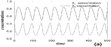
FIG. 1.: (a) The Mean Field Approximation concentrations $x_{1}(t)$ and $x_{2}(t)$ for $(x_{1}(0),x_{2}(0),s(0))$ $=(0.5,0.4,0.1)$, and $(k_{1},k_{2},k_{s})$ $=(0.9,0.3,0.1)$. (b) Monte-Carlo simulations; the solid (dotted) line corresponds to $x_{1}(t)$ over the full lattice (sub-lattice).

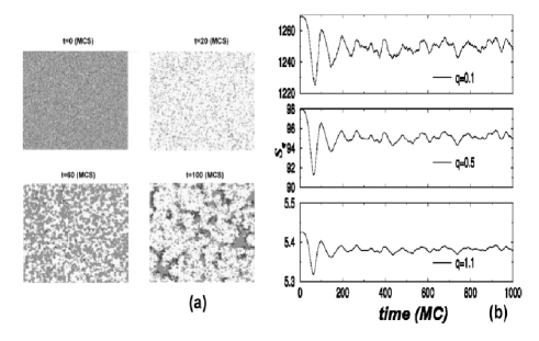
FIG. 2.: (a)Four different snapshots during the evolution of LLV for random uniform initial conditions on a $L=500$ square lattice at the “domain formation mode”; $(k_{1},k_{2},k_{s})=(0.9.0.3,0.1)$. (b)$S_{q}(t)$ with $l=10$.

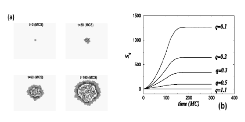
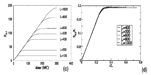
FIG. 3.: (a) Four different snapshots during the evolution of a system covered initially by $S$ with one small mixed droplet. The system linear size is $L=500$ while the droplet size is $l=8$; $(k_{1},k_{2},k_{s})=(1.0,1.0,1.0)$. (b)$S_{q}(t)$. (c)$S_{0.5}(t)$ for various lattice sizes. (d) Collapse of the Fig. 3c data.

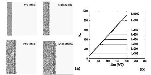
FIG. 4.: (a) Four snapshots of the LLV model at the “stripe growth” mode; $(k_{1},k_{2},k_{s})$ $=(1.0,1.0,1.0)$. (b)$S_{0}(t)$ for $500\times L$ lattices.

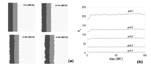
FIG. 5.: (a)Four different snapshots during the evolution of a $L=500$ lattice containing initially two stripes of size $50\times 500$; $(k_{1},k_{2},k_{s})$ $=(1.0,1.0,1.0)$. (b)$S_{q}(t)$.

REFERENCES

- [1] C. Tsallis, J. Stat. Phys. 52, 479 (1988); E. M. F. Curado and C. Tsallis, J. Phys. A 24, L69 (1991) [Corrigenda: 24, 3187 (1991) and 25, 1019 (1992)]; C. Tsallis, R.S. Mendes and A.R. Plastino, Physica A 261, 534 (1998).
- [2] S. Abe and Y. Okamoto, eds., Nonextensive Statistical Mechanics and its Applications, Series Lecture Notes in Physics (Springer-Verlag, Berlin, 2001); G. Kaniadakis, M. Lissia and A. Rapisarda, eds., Non Extensive Statistical Mechanics and Physical Applications, Physica A 305, No 1/2 (Elsevier, Amsterdam, 2002); M. Gell-Mann and C. Tsallis, eds., Nonextensive Entropy - Interdisciplinary Applications (Oxford University Press, 2003), in preparation. An updated bibliography can be found at the web site http://tsallis.cat.cbpf.br/biblio.htm
- [3] A. R. Plastino and A. Plastino, Phys. Lett. A 174, 384 (1993); A.R. Plastino, in Nonextensive Statistical Mechanics and Its Applications, eds. S. Abe and Y. Okamoto (Springer, Berlin, 2001).
- [4] I. Bediaga, E.M.F. Curado and J. Miranda, Physica A 286, 156 (2000).
- [5] C. Beck, Phys. Rev. Lett. 87, 180601 (2001); N. Arimitsu and T. Arimitsu, Europhys. Lett. 60, 60 (2002); M. Peyrard and I. Daumont, Europhys. Lett. bf 59, 834 (2002); A.M. Reynolds, Phys. Fluids 14, 1442 (2002) and 15, L1 (2003).
- [6] A. Upadhyaya, J.-P. Rieu, J.A. Glazier and Y. Sawada, Physica A 293, 549 (2001).
- [7] P. A. Alemany and D. H. Zanette, Phys. Rev. E 49, R956 (1994); C. Tsallis, S. V. F. Levy, A. M. C. Souza and R. Maynard, Phys. Rev. Lett. 75, 3589 (1995).
- [8] A.R. Plastino and A. Plastino, Physica A 222, 347 (1995).
- [9] M. L. Lyra and C. Tsallis, Phys. Rev. Lett. 80, 53 (1998); E.P. Borges, C. Tsallis, G.F.J. Ananos and P.M.C. deOliveira, Phys. Rev. Lett. 89, 254103 (2002).
- [10] Y.S. Weinstein, S. Lloyd and C. Tsallis, Phys. Rev. Lett. 89, 214101 (2002).
- [11] V. Latora, A. Rapisarda and C. Tsallis, Phys. Rev. E 64, 056134 (2001).
- [12] L. Borland, Phys. Rev. Lett. 89, 098701 (2002).
- [13] F. A. Tamarit, S. A. Cannas and C. Tsallis, Eur. Phys. J. B 1, 545 (1998).
- [14] S. Tong, A. Bezerianos, J. Paul, Y. Zhu and N. Thakor, Physica A 305, 619 (2002).
- [15] A. Provata, G. Nicolis and F. Baras, J. Chem. Phys. 110, 8361 (1999).
- [16] A. J. Lotka, Proc. Nat. Acad. Sci. USA, 6, 410 (1920); V. Volterra, Lecons sur la theorie mathematique de la lutte pour la vie, Gauthier-Villars, Paris, 1936.
- [17] G. A. Tsekouras and A. Provata, Phys. Rev. E 65, 016204 (2002).
- [18] G. Picard and T. W. Johnston, Phys. Rev. Lett. 48, 1610 (1982).