Fractional-quantum-Hall edge electrons and Fermi statistics

Abstract

We address the quantum statistics of electrons created in the low-energy edge-state Hilbert space sector of incompressible fractional quantum Hall states, considering the possibility that they may not satisfy Fermi statistics. We argue that this property is not a priori obvious, and present numerical evidence based on finite-size exact-diagonalization calculations that it does not hold in general. We discuss different possible forms for the expression for the electron creation operator in terms of edge boson fields and show that none are consistent with our numerical results on finite-size $\nu=2/5$ states with short-range electron-electron interactions. Finally, we discuss the current body of experimental results on tunneling into quantum Hall edges in the context of this result.

I Introduction

The quantum Hall (QH) effect Prange and Girvin (1990); MacDonald (1995) occurs when an incompressibility, i.e., a discontinuity in the dependence of chemical potential $\mu$ on density, occurs at a two-dimensional (2D) electron system (ES) sheet density $n_{0}$ that is magnetic-field $B$ dependent. The QH effect at integer Landau-level filling factors $\nu=2\pi\ell^{2}n_{0}$ arises from the quantization of 2D ES kinetic energy and from the macroscopic degeneracy of Landau-level states with a particular kinetic energy. ($\ell=\sqrt{\hbar c/|eB|}$ is known as the magnetic length.) The fractional QH effect (chemical potential jumps at fractional values of $\nu$), on the other hand, does not occur in a non-interacting electron system, and is due to constraints on the correlationsLaughlin (1983) that can be achieved among electrons that have the same quantized kinetic energy. A necessary consequenceMacDonald (1995) of magnetic-field dependence in $n_{0}$ is the existence of states in the chemical-potential gap that are localized at the edge of a finite-size system and carry equilibrium current $I$ with the property $dI/d\mu=\nu e/h$.Laughlin (1981) These edge-electron systems are obviously one-dimensional and, since they carry an equilibrium current, obviously chiral.Fröhlich and Zee (1991) Microscopically,Halperin (1982) the edge of a non-interacting electron system at integer filling factor $\nu=m$ is equivalent, at low energies, to a one-dimensional electron system with $m$ flavors of fermions that can travel only in one direction, i.e., $m$ chiral fermion branches. It was argued some time ago,MacDonald (1990); Wen (1990) on the basis of trial wavefunctions for finite-size systems, that the edges of incompressible fractional QH states can also be described microscopically as chiral one-dimensional electron fluids that have, in general, an unequal number of inequivalent left-moving and right-moving branches. In a series of beautiful papers based on hydrodynamic and field-theoretic considerations, WenWen (1990, 1992, 1995) proposed and developed the idea that the properties of fractional QH edges could be described using a generalization of the bosonization approach that was developed earlier for conventional one-dimensional electron systemsSchotte and Schotte (1969); Luther and Peschel (1974); Emery (1979); Voit (1994) and provides a simple description of their characteristicHaldane (1981) Luttinger-liquid power-law correlation functions. In Wen’s theory, edge excitations can be described microscopically in terms of a number of chiral boson fields, and the resulting edge system is a chiral Luttinger liquid ($\chi$LL). Finite-size numerical calculations Palacios and MacDonald (1996) have been a useful tool in verifying the fundamentally bosonic character of the edge-excitation spectrum and in testing some experimental predictions of $\chi$LL theory. Further experimental evidence in support of some aspects of $\chi$LL theory is summarized below. There are, however, difficulties in reconciling this effort to capture generic aspects of the microscopic physics of fractional QH edges with experimental observations. Early workChang et al. (1996) did appear to imply that the edge structure of QH systems at the Laughlin series of filling factors, i.e., for $\nu=1/(2p+1)$ with positive integer $p$, is rather well-described in terms of a single-branch $\chi$LL characterized by a power-law exponent $\alpha=1/\nu$, as expected on the basis of $\chi$LL considerations. Recently, however, this universal dependence of $\alpha$ on filling factor has been questioned both theoreticallyGoldman and Tsiper (2001); Tsiper and Goldman (2001); Mandal and Jain (2001); Wan et al. (2002) and experimentally.Hilke et al. (2001) In addition, tunneling density-of-states observationsGrayson et al. (1998) at hierarchical filling factors, i.e., $\nu=m/(2mp\pm 1)$ with integer $m>1$ are in apparent contradiction with the predictionsKane and Fisher (1995) of $\chi$LL theory.

Motivated by this stark experimental discrepancy, we re-examine in this paper a key ansatz of $\chi$LL theory, which has appeared to us to be non-obviousZülicke and MacDonald (1999) and concerns the properties of the operator $\tilde{\psi}^{\dagger}$ obtained from the full microscopic electron creation operator $\psi^{\dagger}$ by projecting onto the low-energy sector of edge excitations:

$$\tilde{\psi}^{\dagger}={\mathcal{P}}\,\psi^{\dagger}\,{\mathcal{P}}\quad,$$ (1)

where ${\mathcal{P}}=\sum_{\{\eta_{i}\}}\left|\,\{\eta_{i}\}\right\rangle\left\langle\{\eta_{i}\}\,\right|$ is the projection operator onto the Fock-space subset of low-energy (edge) excitations $\left|\,\{\eta_{i}\}\right\rangle$, discussed at greater length below. In applying $\chi$LL theory to evaluate electronic correlation functions, the representation of $\tilde{\psi}$ in terms of bosonic edge-density fluctuations is a key ingredient. Such bosonization identities can be derived constructivelyShankar (1995); Schönhammer (1997); von Delft and Schoeller (1998) for a conventional one-dimensional electron system.Voit (1994) Their generalization to the fractional-QH case,Wen (1992); Stone and Fisher (1994) in which there is no adiabatic connection to non-interacting electron states, must however be based on appealing but heuristic physical arguments that, ultimately, have to be verified by experiment, or by numerical calculations. In our view it is not clear beyond any doubt that the bosonized forms of $\tilde{\psi}$ that have been used in $\chi$LL theory to evaluate electronic correlation functions and predict observables, like the power-law exponents in tunneling current-voltage characteristics, are always correct. In particular, an important guiding principle that has been used to limit possible bosonized expressions for electron field operators in $\chi$LL theory is the seemingly obvious requirement that they satisfy Fermi statistics. In this paper, we use finite-size exact diagonalization studies of a short-range-interaction model to directly test the Fermi-statistics ansatz. The subset of Fock-space states that represent edge excitations of this model can, for the most part, be identified convincingly. We demonstrate by explicit calculation of some anticommutator matrix elements that electron creation operators projected onto this low-energy Fock space do not satisfy Fermi anticommutation rules. In Section II of this paper, the numerical calculations that support this claim are described in detail. Section III discusses the problem of understanding the properties of the projected electron creation operator and of finding a useful expression for it in terms of edge boson fields, in light of our numerical finding. We conclude in Section IV with a brief summary. A preliminary report on this work was presented earlier.Palacios et al. (2000)

II Numerical test of the Fermi statistics ansatz

The second-quantized operator $\psi^{\dagger}(x,y)$ [$\psi(x,y)$] that creates [annihilates] 2D electrons in the lowest Landau level obeys anticommutation relations that encode the fundamental antisymmetry condition satisfied by many-fermion wavefunctions:

$$\left\{\psi^{\dagger}(x,y),\psi^{\dagger}(x^{\prime},y^{\prime})\right\}=0\quad.$$ (2)

The question we address in this section is whether the anticommutation relations are still satisfied after projection onto the low-energy (long-wavelength) sectors of Fock-space that represent edge excitations of particular incompressible states. Because of the projection, Eq. (2) does not mathematically guarantee the relation

$$\tilde{\psi}^{\dagger}(x,y)\tilde{\psi}^{\dagger}(x^{\prime},y^{\prime})=-\tilde{\psi}^{\dagger}(x^{\prime},y^{\prime})\tilde{\psi}^{\dagger}(x,y)\quad.$$ (3)

A physical argument along the following lines does, however, appear plausible. It is possible to add two different electrons to the system at low energies that are localized at different positions along the edge via processes that can be represented by the projected creation operator. The edge-electron positions can then be adiabatically interchanged, ending up with an equivalent many-fermion state that must differ only by a sign from the original state. If the many-particle state can be represented, at all intermediate relative positions, by two projected creation operators acting on the starting state, it seems hard to escape the conclusion that these operators must satisfy Fermi statistics. However, the correlations that establish the bulk gap could be disturbed when the two electrons are in close proximity. It is therefore difficult to exclude the possibility that this argument breaks down at the crossing point in the exchange path. Related arguments can be advanced in which the exchange paths involve particle creation at different times, but do not appear to us to be conclusive. Our inability to settle this point on the basis of simple general arguments has motivated the numerical calculations we now explain.

The identification of the set of states as edge excitation states of a particular incompressible state in a finite-size many-fermion spectrum is both a challenge and an important source of uncertainty for the conclusions we reach. For $\nu=1/(2p+1)$, the identification is accomplishedPalacios and MacDonald (1996) by appealing to LaughlinLaughlin (1983); MacDonald and Murray (1985) to conclude that the low-energy edge-excitation states appear at angular momenta above $L_{0}=(2p+1)N(N-1)/2$, and that the dimension of subspaces at fixed angular momentum is related to their excess momentum by counting the number of modes in a chiral boson Hilbert space;MacDonald (1996) i.e., one state with angular momentum 1, two with angular momentum 2, three with angular momentum 3, five with angular momentum 4, et cetera. Previous numerical workPalacios and MacDonald (1996) has verified $\chi$LL predictions for $\nu=1/(2p+1)$ edges, but not at filling factors within the range $1/3<\nu<1$, where experiment and theory appear to be at odds.

Incompressibilities at many other values of the filling factor, e.g., for $\nu=m/(2mp\pm 1)$ with positive integer $m$, have been explained using various hierarchical schemesHaldane (1983); Halperin (1984) and using composite-fermion theory.Jain (1989) Composite-fermion theory and variational wavefunctions based on hierarchy-theory ideas make identical predictionsRead (1990) for the values of total angular momentum $L_{0}$ at which maximum-densityMacDonald (1996) incompressible states (those with edge subsystems in their ground states) appear and for the number and chirality of the boson branches in their edge-excitation spectra. For practical reasons explained more fully below, we limit our study to QH systems with two branches of edge excitations that have the same chirality, i.e., that propagate along the edge in the same direction and have, for our circular droplets, excess angular momenta of the same sign. This is the case for QH systems at filling factors $\nu=2/(4p+1)$ where the edge spectrum is expected to be that of two boson modes that share the same chirality.

The angular-momentum values at which maximum-density states occur depend on the number of electrons $N$, and the number of particles to be transferred from the ground to the upper composite-fermion Landau level $N_{qp}$. This notation is chosen to suggest the analogous hierarchy-picture description of the same states, which makes identical predictions for the set of angular-momentum values at which maximum-density states occur. In the composite-fermion language, the number of particles in the lower composite-fermion Landau level is $N-N_{qp}$, and maximum-density finite-size $\nu=2/(4p+1)$ states appear at $L_{0}=(N_{qp}-1)*(N_{qp}-2)/2+(N-N_{qp})(N-N_{qp}-1)/2+2pN(N-1)$, where the last term comes from the Jastrow factor in Jain’s variational wavefunctions and the first term reflects the reduced angular momentum of higher Landau-level states.Dev and Jain (1992) Changing $N_{\text{qp}}$ and/or $N$ is analogous to a topological or zero-mode excitation in a finite-size one-dimensional electron system.Haldane (1981) We denote the N-electron state with $N_{\text{qp}}$ quasiparticles and an edge-density sub-system in its ground state by $\left|\,N,N_{\text{qp}},0\right\rangle$, and its total momentum by $L_{\text{0}}(N,N_{\text{qp}})$. The following relation can be derived from the above composite-fermion expression or from hierarchy theory:

$$L_{0}(N,N_{\text{qp}})=(2p+1)\frac{N(N-1)}{2}+N_{\text{qp}}(N_{\text{qp}}-1)-N\,N_{\text{qp}}\,.$$ (4)

Table 1: Total angular momenta $L_{0}(N,N_{\text{qp}})$ for the ground state of compact fractional-QH systems as predicted from Eq. (4) for $p=1$. These states can be regarded as $N$-electron states in the lowest Landau level that consist of a QH droplet at filling factor $1/3$ supporting a compact daughter droplet of $N_{\text{qp}}$ quasiparticles. In an equivalent description, these are $N$-composite-fermion states with lowest and first-excited composite-fermion Landau levels having occupation $N-N_{\text{qp}}$ and $N_{\text{qp}}$, respectively. Numbers in bold type indicate that the corresponding ground state in our numerical spectra was positively identified as a finite-size $\nu=2/5$ QH state. The ground states whose edge-excitation sectors are explicitly used here to test the Fermi statistics ansatz are indicated by asterisks.

	$N$	5	6	7	8	9	10
$N_{\text{qp}}$
0		30	∗45	63	84	108	135
1		25	39	56	76	99	125
2		22	∗35	∗51	∗70	∗92	117
3			33	48	∗66	∗87	111
4					64	84	107
5							105

For the case $p=1$, Table 2 shows $L_{0}(N,N_{\text{qp}})$ for these finite-size maximum-density states. Finite-size numerical spectra for small $N$ exhibit non-degenerate ground states at these values of $L$, and a low-energy excitation spectrum at small excess $L$ that corresponds to the expected chiral two-branch edge when $N_{qp}$ is close enough to $\approx N/2$. (A chiral two-branch edge has two low-energy states with excess angular momentum equal to 1, five with excess angular momentum 2, ten with excess momentum 3, et cetera. As an example, Figure 1 shows spectra obtained for $N=8$ and $9$ particles.) We define the edge-state Fock-space projection ${\mathcal{P}}$ by retaining for each $N$ and $N_{\text{qp}}$ only these states.

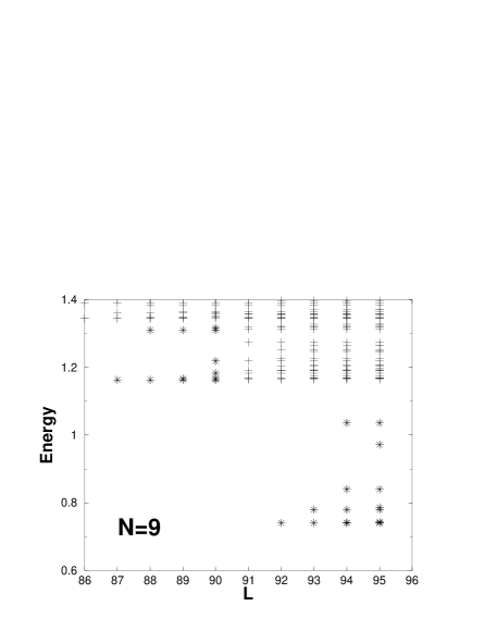
Figure 1: Low-energy portion of the exact finite-size spectrum for $N=8$ and $N=9$ particles with short-range interactions. The non-degenerate states at $L=70$ ($N=8$), $L=87$ ($N=9$), and $L=92$ ($N=9$) can be identified as maximum-density ground states of a $\nu=2/5$ finite-size QH droplet. Their energy is separated by a large gap from a continuum of bulk-excited states. States at higher angular momenta with energies below that gap (indicated by asterisks) can be unambiguously identified as edge excitations. Note that the multiplicity of these states at $L=71$ and $L=72$ in the left panel and $L=88$, $93$, and $94$ in the right panel is exactly as expected for a two-branch chiral boson system. For $L\geq 73$ in the left panel and $L\geq 89$ and $L\geq 95$ in the right panel, ‘edge’ states exist that have energies as high as bulk excitations. In the calculations described below, we try to select anticommutator matrix elements that do not require us to utilize Fock-space sectors with missing edge states. Cases for which there are missing states are explicitly identified in our discussion. The energies plotted here do not include the contribution, proportional to total angular momentum, from our model’s parabolic confinement potential which lifts the energies of states with larger $L$. The ground state is determined by the strength of this confinement potential. In the thermodynamic limit, it will be one of the $\nu=2/5$ maximum-density-droplet states when the chemical potential lies in the $\nu=2/5$ gap.

The low-energy Fock space is then the direct sum of the low-energy Hilbert spaces for different particle numbers $N$; each of these is in turn the direct sum of orthogonal subspaces labeled by different values of $N_{\text{qp}}$, the number of composite fermions in the first excited Landau level. Our understanding of $\chi$LL theory is that it attempts to describe the physics of QH systems projected onto this subspace. It will prove useful to write the projected electron creation operator as the sum of separate contributions labeled by the change in the number of quasiparticles that accompanies a particle addition. We therefore write $\tilde{\psi}^{\dagger}=\sum_{n}\tilde{\psi}^{\dagger}_{n}$ where the operator $\tilde{\psi}^{\dagger}_{n}$ changes $N_{\text{qp}}$ by $n$. In other words, an electron can be added to an $N$-particle, $N_{\text{qp}}$-quasiparticle finite-size state in many different ways, distinguished both by the resulting edge disturbance and by the number of quasiparticles in the resulting $(N+1)$-particle state. If the corresponding projected electron creation operators $\tilde{\psi}^{\dagger}_{n}$ satisfy Fermi statistics, their anticommutator $\{\tilde{\psi}_{n^{\prime}}^{\dagger},\,\tilde{\psi}_{n}^{\dagger}\}$ will vanish identically. We check for Fermi statistics by evaluating anticommutator matrix elements that involve the lowest possible excess momenta and are therefore likely to have the smallest finite-size effects. In particular, we define

$$A_{n,n^{\prime}}(N,N_{\text{qp}}) = \left\langle N+2,N_{\text{qp}}+n+n^{\prime},0\,\right|c^{\dagger}_{K_{2}}{\mathcal{P}}_{N+1,N_{\text{qp}}+n}\,c^{\dagger}_{K_{1}}\left|\,N,N_{\text{qp}},0\right\rangle\quad,$$ (5a)

$$B_{n,n^{\prime}}(N,N_{\text{qp}}) = \left\langle N+2,N_{\text{qp}}+n+n^{\prime},0\,\right|c^{\dagger}_{K_{1}}{\mathcal{P}}_{N+1,N_{\text{qp}}+n^{\prime}}\,c^{\dagger}_{K_{2}}\left|\,N,N_{\text{qp}},0\right\rangle\quad,$$ (5b)

with $K_{1}=K_{\text{F}}^{(n)}(N,N_{\text{qp}})$ and $K_{2}=K_{\text{F}}^{(n^{\prime})}(N+1,N_{\text{qp}}+n)$ where $K_{\text{F}}^{(n)}(N,N_{\text{qp}}):=L_{0}(N+1,N_{\text{qp}}+n)-L_{0}(N,N_{\text{qp}})$. The projector ${\mathcal{P}}_{N,N_{\text{qp}}}$ projects onto the subspace of the $N$-particle low-energy subspace having $N_{\text{qp}}$ quasiparticles (i.e., composite fermions in their first excited Landau level). It is then obvious that

$$A_{n,n^{\prime}}(N,N_{\text{qp}}) = \left\langle N+2,N_{\text{qp}}+n+n^{\prime},0\,\right|c^{\dagger}_{K_{2}}\left|\,N+1,N_{\text{qp}}+n,0\right\rangle\left\langle N+1,N_{\text{qp}}+n,0\,\right|c^{\dagger}_{K_{1}}\left|\,N,N_{\text{qp}},0\right\rangle\quad,$$

$$B_{n,n^{\prime}}(N,N_{\text{qp}}) = \sum_{\{\eta\}}\left\langle N+2,N_{\text{qp}}+n+n^{\prime},0\,\right|c^{\dagger}_{K_{1}}\left|\,N+1,N_{\text{qp}}+n^{\prime},\{\eta\}\right\rangle\left\langle N+1,N_{\text{qp}}+n^{\prime},\{\eta\}\,\right|c^{\dagger}_{K_{2}}\left|\,N,N_{\text{qp}},0\right\rangle\,,$$

where $\left|\,N+1,N_{\text{qp}}+n^{\prime},\{\eta\}\right\rangle$ are edge excitations in the $(N+1)$-particle, $(N_{\text{qp}}+n^{\prime})$-quasiparticle system for excess total momentum

$$\Delta K_{\text{F}}^{(n,n^{\prime})} = K_{\text{F}}(N+1,N_{\text{qp}}+n,n^{\prime})-K_{\text{F}}(N,N_{\text{qp}},n^{\prime})\,,$$ (7)

$$= 2p+1+2nn^{\prime}-n-n^{\prime}\quad.$$

Fermi statistics is satisfied if the ratio $B/A$ equals $-1$.

Table 2: Results for the ratio between the matrix elements $A=\langle L_{0}^{(N+2)}|c^{\dagger}_{K_{2}}{\mathcal{P}}\,c^{\dagger}_{K_{1}}|L_{0}^{(N)}\rangle$ and $B=\langle L_{0}^{(N+2)}|c^{\dagger}_{K_{1}}{\mathcal{P}}\,c^{\dagger}_{K_{2}}|L_{0}^{(N)}\rangle$. This ratio should always equal $-1$ if the edge–electron operator satisfies Fermi statistics. We have chosen values $K_{1}$ and $K_{2}$ such that $A=\langle L_{0}^{(N+2)}|c^{\dagger}_{K_{2}}|L_{0}^{(N+1)}\rangle\langle L_{0}^{(N+1)}|c^{\dagger}_{K_{1}}|L_{0}^{(N)}\rangle$ involves matrix elements between maximum-density states only. When the order of edge–electron operators is reversed, $B=\sum_{r}\langle L_{0}^{(N+2)}|c^{\dagger}_{K_{1}}|{\tilde{L}}_{r}^{(N+1)}\rangle\langle{\tilde{L}}_{r}^{(N+1)}|c^{\dagger}_{K_{2}}|L_{0}^{(N)}\rangle$, with the sum ranging over matrix elements between edge states $|{\tilde{L}}_{r}^{(N+1)}\rangle$ with excess angular momentum $\Delta K=L_{0}^{(N)}+K_{2}-{\tilde{L}}_{0}^{(N+1)}$. The first block corresponds to $B_{0,0}/A_{0,0}$, the second to $B_{0,1}/A_{0,1}$ and $B_{1,0}/A_{1,0}$, and the third to $B_{1,1}/A_{1,1}$.

$N$	$L_{0}^{(N)}$	$L_{0}^{(N+1)}$	$L_{0}^{(N+2)}$	$K_{1}$	$K_{2}$	${\tilde{L}}_{0}^{(N+1)}$	$\Delta K$	$B/A$
5	30	45	63	15	18	45	3	$-1$
5	22	35	51	13	16	35	3	$-0.78$
6	35	51	70	16	19	51	3	$-0.99$
7	51	70	92	19	22	70	3	$-1.02$
8	70	92	117	22	25	92	3	$-1.01$
8	66	87	111	21	24	87	3	$-1.05$
6	39	56	70	17	14	51	2	$-1.12$
7	56	76	92	20	16	70	2	$-0.95$
7	51	66	87	15	21	70	2	$-1.24$
7	51	70	87	19	17	66	2	$-1.32$
8	70	92	111	22	19	87	2	$-1.14$
8	70	87	111	17	24	92	2	$-1.11$
8	76	99	117	23	18	92	2	$-0.88$
6	39	51	66	12	15	51	3	$-1.44$
7	56	70	87	14	17	70	3	$-1.26$
8	76	92	111	16	19	92	3	$-1.20$

Our numerical results are summarized in Table 2. We start by considering a QH droplet at filling factor $1/3$, i.e., states with $N_{qp}=0$. (See the first row in Table 2.) Although only one case is presented there, it turns out that for any finite-size system with short-range interactions, the electron operator projected onto the subspace of low-energy excitations above the ground state at $\nu=1/3$ satisfies Fermi statistics exactly. The Fermi statistics of edge excitations is a property of Laughlin many-body wavefunctions,Laughlin (1983) which are exact in the case of the hard-core-interaction model at $\nu=1/(2p+1)$.Palacios (2002) It is apparent from the remaining entries in Table 2 that this property of hard-core-model single-branch QH edges does not, in general, hold in the $\nu=2/5$ two-branch case. We have tested edge-excitation subspaces for systems with $N=6,7,8$, and $9$ electrons and find that the ratio $B/A$ that ‘measures’ Fermi statistics often differs substantially from $-1$. Instead, a strong dependence of $B/A$ on the change in $N_{qp}$ that accompanies particle addition is apparent from our data. For example, consider the sequences $L^{(N)}$–$L^{(N+1)}$–$L^{(N+2)}$ where particles are added without adding hierarchy quasiparticles. In composite-fermion language, this corresponds to adding electrons to the lowest composite-fermion Landau level only. The finite sequences in this class that we have studied, e.g., 35–51–70, 51–70–92, and 66–87–111, are gathered in the first block of Table 2. Although violations of Fermi statistics are numerically unambiguous, they are large only for those cases where the edge sector is seriously incomplete (only 5 out of 10 edge states could be identified in the L=38 sector for the sequence 22–35–51). To some extent, this result is not surprising since the addition of an electron to the lowest composite-fermion Landau level is expected to involve excitations of this level only, as in the $\nu=1/3$ case. It seems plausible that the results should be similar. The deviation from Fermi statistics is suspicious, however, when contrasted with the perfect accuracy seen for the $\nu=1/3$ QH droplet. When an anticommutator involving $\tilde{\psi}^{\dagger}_{1}$ (increasing the number of higher-Landau-level composite fermions by one) is considered, as in the sequences 39–51–66, 56–70–87, and 76–92-111 (see the third block in Table 2), the deviations from Fermi statistics are larger. Note that some of the same finite-size edge states are used here and in the $\tilde{\psi}^{\dagger}_{0}$ case for which Fermi statistics is more closely approximated. It is important to recognize, however, that the edge sectors used in all these sequences are not complete even for the larger systems considered. The incompleteness is related to the fact that there are only two electrons in the first excited composite-fermion Landau level which implies that the daughter droplets are substantially smaller than the parent droplets, exacerbating finite-size difficulties. The strongest evidence that Fermi-statistics relations are not satisfied comes from the remaining sequences in Table 2, for which the numerical edge-state sector is usually complete. There is no unique way of estimating a thermodynamic limit for $B/A$ from our data. A consistent scheme would have to keep $N-2N_{\text{qp}}\ll N$ as $N\rightarrow\infty$, in order to maintain parent and daughter fluids that are similar in size. The small system sizes tractable using current numerical methods render such an extrapolation impossible. Examining the trends in Table 2, however, we are reasonably confident that differences $|1+B/A|>0.05$ are significant and not merely due to finite-size effects. We note that in the case of conventional one-dimensional electron systems, a corresponding calculation would always result in exact conformation with Fermi statistics; there are no finite-size corrections. The $\nu=1/3$ hard-core-model case also produces results in agreement with Fermi statistics without finite-size corrections. In contrast, our calculations exhibit large deviations from Fermi statistics for many sequences where the edge states expected for a two-branch boson system are clearly resolved in the spectrum, not only for those with an incomplete edge sector. This is the case for 51–66–87 for example. Furthermore, when edge states exist that have energies above the gap for bulk excitations and can no longer be clearly identified (this is the case, e.g., for 8-particle states at total momentum 73), the value of $B/A$ turns out to be determined almost entirely by contributions from edge states with energies below the gap. Inclusion of any number of states (bulk or edge) above the gap energy changes $B/A$ only by a few percent. Finally, deviations from Fermi statistics do not seem to diminish with increasing particle number. On the contrary, the more unambiguously identified edge-state sectors at larger $N$ yield values of $B/A$ that differ consistently from $-1$, especially for anticommutators involving the component of the creation operator that increases the number of daughter quasiparticles, $\tilde{\psi}_{1}^{\dagger}$.

III Properties of Candidate Bosonized Electron Operators

Our numerical results clearly support a multi-branch chiral-boson form for the excitation spectrum of a fractional-QH edge, but raise new questions about the representation of projected electron creation operators in terms of these boson fields. This issue is discussed in the following section. We start by carefully examining the arguments that have been made in $\chi$LL theory to obtain bosonization identities. Some of these heuristic arguments must be ruled out if the edge projection of the electron operator does indeed not satisfy Fermi statistics. Alternative proposals are discussed, but we have not been able to find a simple form that is consistent with our numerical results, suggesting that the true expression may not be universal.

In a conventional one-dimensional system,Voit (1994) the low-energy projection of the electron operator $\psi^{\dagger}_{\text{1D}}$ is expressed as the sum $\tilde{\psi}_{\text{1D}}^{\dagger}=\tilde{\psi}_{\text{R}}^{\dagger}+\tilde{\psi}_{\text{L}}^{\dagger}$ of right-moving and left-moving chiral fermion contributions $\tilde{\psi}_{\text{R,L}}^{\dagger}$. For these chiral fermion operators, an identity relating them to the bosonic charge fluctuations of an interacting system can be derived rigorously.Shankar (1995); Schönhammer (1997); von Delft and Schoeller (1998) Fractional-QH edges do appear to be realizations of chiral one-dimensional systems, as indicated by the multiplicity of low-lying many-electron states in our numerically obtained spectra. Given this observation, one is tempted to push the analogy further and search for a bosonization identity for the projected edge-electron operators $\tilde{\psi}_{n}^{\dagger}$. Assuming that it is local in the angular coordinate $\theta$ along the edge, it should read

$$\tilde{\psi}^{\dagger}_{n}(\theta)=\sqrt{z}\,e^{-i\theta K_{\text{F}}^{(n)}(\hat{N},\hat{N}_{\text{qp}})}e^{-i\phi_{n}^{\dagger}(\theta)}e^{-i\phi_{n}(\theta)}\,{\mathcal{U}}_{n}^{\dagger}\quad,$$ (8)

where $z$ denotes a normalization constant. The ‘Klein factor’ ${\mathcal{U}}_{n}^{\dagger}$ is a ladder operator that connects many-particle ground states, ${\mathcal{U}}_{n}^{\dagger}\left|\,N,N_{\text{qp}},0\right\rangle=\left|\,N+1,N_{\text{qp}}+n,0\right\rangle$ and commutes with bosonic edge-density operators. The correct commutation relations for operators with different $n$, whatever they are, have to be encoded in these factors. The chiral phase field $\phi_{n}(\theta)$ is a superposition of edge-density fluctuations. For $\nu=2/(4p+1)$, the following decomposition of the phase field in terms of eigenmodes is always possible:

$$\phi_{n}(\theta)=\frac{1}{\sqrt{\nu}}\,\phi^{\text{(c)}}(\theta)+\xi_{n}\,\phi^{\text{(n)}}(\theta)\quad,$$ (9)

were $\phi^{\text{(c)}}$ is the phase field of the charged edge-magnetoplasmon mode which corresponds to fluctuations in the total edge-charge density, and $\phi^{\text{(n)}}$ is its orthogonal complement, the so-called neutral mode. The prefactor $1/\sqrt{\nu}$ of the charged mode in Eq. (9) is mandated by the fact that the addition of an electron necessarily increases total electric charge by unity. Additional assumptions are necessary, however, to fix the values of $\xi_{n}$.

Within $\chi$LL theory,Wen (1992) the operators $\tilde{\psi}_{0}$ and $\tilde{\psi}_{2p+1}$ are believed to be special in that they create electrons localized at the putative ‘outer’ and ‘inner’ edges which are the boundaries of the outer parent and inner daughter QH droplets with filling factors $\nu_{\text{o}}=1/(2p+1)$ and $\nu_{\text{i}}=1/[(2p+1)(4p+1)]$, respectively, that comprise the $\nu=2/(4p+1)$ QH state. The density fluctuations at the ‘outer’ and ‘inner’ edges are given by $(\nu_{\text{o}}/L)\,\partial_{\theta}\phi_{0}$ and $(\nu_{\text{i}}/L)\,\partial_{\theta}\phi_{2p+1}$, respectively, and the definition of charged and neutral modes implies that

$$\phi^{\text{(c)}} = \frac{1}{\sqrt{\nu}}\left(\nu_{\text{i}}\,\phi_{2p+1}+\nu_{\text{o}}\,\phi_{0}\right)\quad,$$ (10a)

$$\phi^{\text{(n)}} = \sqrt{\frac{\nu_{\text{o}}\nu_{\text{i}}}{\nu}}\left(\phi_{2p+1}-\phi_{0}\right)\quad.$$ (10b)

The addition of electrons to the edge with concomitant change of $2p+1-n$ flux quanta is viewed as adding the electron to the ‘outer’ edge and transferring at the same location $n$ fractionally charged quasiparticles from the outer QH droplet to the inner one. This suggests the relation $\tilde{\psi}_{n}^{\dagger}\sim\tilde{\psi}_{0}^{\dagger}\,\exp\{in\nu_{\text{o}}(\phi_{0}-\phi_{2p+1})\}$ which is equivalent to

$$\xi_{n}=\frac{1}{\sqrt{2}}\,(2n-1)\quad.$$ (11)

The chain of arguments leading to Eq. (11) involves several assumptions that are not obviously satisfied. For example, it is not clear why changes in $N_{qp}$ that accompany electron addition have to occur by transferring localized quasiparticles from an ‘inner’ edge to an ‘outer’ one. Relaxing this condition would lift the restriction expressed by Eq. (11). In fact, two of the present authors suggested the different choice $\xi_{n}=0$ for strongly correlated fractional-QH edges.Zülicke and MacDonald (1999) The fact that Eq. (11) ensures Fermi statistics has been regardedLee and Wen as strong support for this line of argument. However, the numerical results discussed in Sec. II suggest that there is no basis for this requirement. Assuming that a simple bosonization identity of the form given in Eq. (8) holds, we can extract the values $\xi_{0}^{2}\approx 0.51\pm 0.02$ and $\xi_{1}^{2}\approx 0.65\pm 0.06$ from the data for matrix elements of anticommutators $\{\tilde{\psi}_{0}^{\dagger},\,\tilde{\psi}_{0}^{\dagger}\}$ and $\{\tilde{\psi}_{1}^{\dagger},\,\tilde{\psi}_{1}^{\dagger}\}$. (See the Appendix for details of the calculation.) The value of $\xi_{1}^{2}$ deviates significantly from that expected within $\chi$LL theory ($1/2$) because $\tilde{\psi}_{1}^{\dagger}$ does not satisfy Fermi statistics. While the standard deviations from the average extracted $\xi_{0,1}^{2}$ are reasonably small, we have to caution the reader by noting that the assumption of a simple bosonization identity would imply symmetry of $B_{n,n^{\prime}}/A_{n,n^{\prime}}$ under exchange $n\leftrightarrow n^{\prime}$. Clearly, no such symmetry is exhibited in our data. The significantly large deviation between $B_{0,1}/A_{0,1}$ and $B_{1,0}/A_{1,0}$ raises a big question mark: unless rather complex features are ascribed to the Klein factors, a consistent interpretation of our data using a local bosonization formula like Eq. (8) is impossible.

IV Discussion and Conclusions

We have shown, by explicit numerical calculation of anticommutator matrix elements, that the projection of the lowest-Landau-level electron creation operator onto the low-energy edge-excitation Fock subspace of a $\nu=2/5$ incompressible quantum Hall state does not satisfy Fermi statistics. We observe a consistent dependence of the anticommutation rules on the particular procedure for adding electrons, i.e., on the change in quasiparticle number that accompanies particle addition. We find that the numerical data cannot be consistently interpreted by assuming any simple generalization of conventional bosonization identities. In particular, the expression for the electron operator solely in terms of rigid edge deformations (magnetoplasmon modes), which two of us argued for previouslyZülicke and MacDonald (1999) on heuristic grounds is also not supported by our calculations. Since our present study was performed for a system with short-range interactions, however, we cannot exclude the possibility that real QH samples where long-range Coulomb interactions are present may be consistently described by such a bosonization identity, as is suggested by the amazing experimental finding that the tunneling-$IV$ exponent $\alpha\approx 1/\nu$.

Our numerical study demonstrates that the specific form of the boson representation of the edge electron creation operator cannot be inferred by postulating Fermi statistics of the projected edge-electron operator. AlternativesZülicke and MacDonald (1999) to the $\chi$LL expressionsWen (1992) cannot be ruled out on these general grounds. However, our present data for the short-range-interacting case supports neither the conventional chiral-Luttinger-liquid picture nor any simple alternative. This points strongly towards the possibility that there is no simple universal local bosonization identity for the edge-electron operator, a conclusion also reached in an independent recent study.Mandal and Jain (2002) If true, this likely implies that electronic properties of fractional-quantum-Hall edges depend crucially on sample specifics.

*

Appendix A Anticommutators calculated from bosonization

Within the bosonization formalism, the quantities $A_{n,n^{\prime}}$ and $B_{n,n^{\prime}}$, defined by Eqs. (5), do not depend on $N$ or $N_{\text{qp}}$. We find $A_{n,n^{\prime}}=z$ and

$$\frac{B_{n,n^{\prime}}}{A_{n,n^{\prime}}}=\chi_{n,n^{\prime}}\sum_{\{\eta\}}\left\langle N+1,N_{\text{qp}}+n^{\prime},0\,\right|e^{-i\phi_{n}(0)}\left|\,N+1,N_{\text{qp}}+n^{\prime},\{\eta\}\right\rangle\left\langle N+1,N_{\text{qp}}+n^{\prime},\{\eta\}\,\right|e^{-i\phi_{n^{\prime}}^{\dagger}(0)}\left|\,N+1,N_{\text{qp}}+n^{\prime},0\right\rangle\,,$$ (12)

where $\left|\,N+1,N_{\text{qp}}+n^{\prime},\{\eta\}\right\rangle$ are excited states with excess (boson) momentum equal to $\Delta K_{\text{F}}^{(n,n^{\prime})}$. Contributions from Klein factors are contained in $\chi_{n,n^{\prime}}$ which satisfies $\chi_{n,n}=1$. To better understand the two-branch case, it is useful to first consider the situation when only a single branch of edge excitations is present.

A.1 Single-branch case

At the edge of a QH sample at filling factor equal to $1/(2p+1)$, a single branch of edge excitations exists which corresponds to the edge-magnetoplasmon (charged) mode. [Within the formalism described above, we would have to set $\xi_{n}\equiv 0$, $\phi_{n}=\phi^{\text{(c)}}\equiv\phi$, and let $\nu\to 1/(2p+1)$ in order to describe the single-branch edge.] Denoting by $a^{\dagger}_{Q}$ ($a_{Q}$) the bosonic creation (annihilation) operator for an edge-magnetoplasmon excitation with wave number $Q$, we can give expressions for both the phase field entering the bosonization identity and the excited states appearing in Eq. (12):

$$\phi(\theta) = \frac{1}{\sqrt{\nu}}\sum_{Q>0}\frac{e^{iQ\theta}}{\sqrt{Q}}\,a_{Q}\quad,$$ (13a)

$$\left|\,N+1,0,(l)\right\rangle = \prod_{r}\frac{\big{[}a_{0,r}^{\dagger}\big{]}^{l_{r}}}{\sqrt{l_{r}!}}\left|\,N+1,0,0\right\rangle\quad,$$ (13b)

with $\sum_{r}rl_{r}=\Delta K_{\text{F}}=2p+1$. Here, $r>0$ and $l_{r}\geq 0$ are integers, and $(l)$ is a partition of the integer $\Delta K_{\text{F}}$ labeling possible many-body excited states. Straightforward calculation yields

$$\left\langle N+1,0,0\,\right|e^{-i\phi(0)}\left|\,N+1,0,(l)\right\rangle=\left\langle N+1,0,(l)\,\right|e^{-i\phi^{\dagger}(0)}\left|\,N+1,0,0\right\rangle=\prod_{r}\left[(-\nu\,r)^{l_{r}}\,l_{r}!\right]^{-\mbox{$\textstyle\frac{1}{2}$}}\quad.$$ (14)

Inserting this result into Eq. (12), we find

$$\frac{B}{A} = \sum_{(l)}\prod_{r\in(l)}\left[(-\nu\,r)^{l_{r}}\,l_{r}!\right]^{-1}\quad,$$ (15a)

$$= \frac{(-1)^{\Delta K_{\text{F}}}}{\Delta K_{\text{F}}!}\sum_{s=0}^{\Delta K_{\text{F}}}\left(\frac{1}{\nu}\right)^{s}\sum_{(l)_{s}}{\mathcal{S}}^{(s)}_{\Delta K_{\text{F}}}\quad,$$ (15b)

where $(l)_{s}$ denotes a partition with $s$ cycles, and ${\mathcal{S}}^{(s)}_{\Delta K_{\text{F}}}$ denotes Stirling numbers of the first kind.Abramowitz and Stegun (1972) (Klein factors are irrelevant for calculating $B/A$ of a single-branch edge.) Using relation 24.1.3 from Ref. Abramowitz and Stegun, 1972, and introducing the generalized binomial coefficients,

$$\left(\begin{array}[]{c}a\\ n\end{array}\right)=\frac{\Gamma(a+1)}{\Gamma(a+1-n)n!}\quad,$$

we find

$$\frac{B}{A}=(-1)^{\Delta K_{\text{F}}}\,\,\left(\begin{array}[]{c}\nu^{-1}\\ \Delta K_{\text{F}}\end{array}\right)\quad.$$ (16)

Obviously, because $\nu^{-1}\equiv\Delta K_{\text{F}}=2p+1$, we find that Fermi statistic holds for the bosonized expression of the projected edge–electron operator at Laughlin–series filling factors: $B/A=-1$.

A.2 Two-branch case

Lets now consider again the case $\nu=2/(4p+1)$ where two edge branches with the same chirality are present. Many-body excited states entering Eq. (12) are then the eigenstates of the quadratic edge-density-wave Hamiltonian which are spanned by bosonic operators that are, in general, some orthogonal linear combinations of the charged and neutral-mode excitations. The coefficients in the linear transformation that relate the charged and neutral modes to the bosonic normal modes of the Hamiltonian depend on microscopic details, i.e., the velocities of the charged and neutral modes as well as their coupling via interactions. However, it turns out that we do not need these coefficients explicitly. It suffices to know that the phase fields entering the bosonization formula can be expressed in terms of the normal modes, $\phi_{n}=\sum_{j=1}^{2}\eta_{j}^{(n)}\,\varphi_{j}$, where

$$\eta_{1}^{(n)} = \frac{\cos\alpha}{\sqrt{\nu}}-\xi_{n}\,\sin\alpha\quad,$$ (17a)

$$\eta_{2}^{(n)} = \frac{\sin\alpha}{\sqrt{\nu}}+\xi_{n}\,\cos\alpha\quad.$$ (17b)

The fields $\varphi_{j}$ are defined in terms of the bosonic operators $a_{j,Q}$ that annihilate excitations of the $j$th normal mode in analogy to Eq. (13a), and microscopic details of the edge determine the value of $\alpha$. Excited states entering Eq. (12) are direct products of excited states in the two normal-mode subspaces whose combined excess momenta equals $\Delta K^{(n,n^{\prime})}_{\text{F}}$. Within each of the normal-mode sectors, total excess momentum is partitioned among the possible many-boson states as in the single-branch case. We can, therefore, employ the result (16) and find

$$\frac{B_{n,n^{\prime}}}{A_{n,n^{\prime}}} = \chi_{n,n^{\prime}}\,\,(-1)^{\Delta K^{(n,n^{\prime})}_{\text{F}}}\,\sum_{Q}\left(\begin{array}[]{c}\eta_{1}^{(n)}\eta_{1}^{(n^{\prime})}\\ Q\end{array}\right)\,\left(\begin{array}[]{c}\eta_{2}^{(n)}\eta_{2}^{(n^{\prime})}\\ \Delta K^{(n,n^{\prime})}_{\text{F}}-Q\end{array}\right)\quad,$$ (18e)

$$= \chi_{n,n^{\prime}}\,\,(-1)^{\Delta K^{(n,n^{\prime})}_{\text{F}}}\,\left(\begin{array}[]{c}\eta_{1}^{(n)}\eta_{1}^{(n^{\prime})}+\eta_{2}^{(n)}\eta_{2}^{(n^{\prime})}\\ \Delta K^{(n,n^{\prime})}_{\text{F}}\end{array}\right)\quad.$$ (18h)

Here we have used the addition theorem for generalized binomial coefficients. (See, e.g., Section 12.2 of Ref. Margenau and Murphy, 1956.) Straightforward inspection shows that the sum $\sum_{j}\eta_{j}^{(n)}\eta_{j}^{(n^{\prime})}=\nu^{-1}+\xi_{n}\xi_{n^{\prime}}$ is universal, i.e., independent of $\alpha$. Using that, we can write

$$\frac{B_{n,n^{\prime}}}{A_{n,n^{\prime}}}=\chi_{n,n^{\prime}}\,\,(-1)^{\Delta K^{(n,n^{\prime})}_{\text{F}}}\,\left(\begin{array}[]{c}\nu^{-1}+\xi_{n}\xi_{n^{\prime}}\\ \Delta K^{(n,n^{\prime})}_{\text{F}}\end{array}\right)\quad.$$ (19)

With the choice of values for $\xi_{n}$ according to $\chi$LL theory, which is given in Eq. (11), one finds $\nu^{-1}+\xi_{n}\xi_{n^{\prime}}\equiv\Delta K^{(n,n^{\prime})}_{\text{F}}$. Since $\Delta K^{(n,n)}_{\text{F}}$ is always odd, and with a suitable definition of Klein factorsvon Delft and Schoeller (1998) such that $\chi_{n,n^{\prime}}=(-1)^{n+n^{\prime}}$, one obtains $B/A=-1$.

Two of the authors suggested previously Zülicke and MacDonald (1999) the choice $\xi_{n}=0$. For the special case of $p=1$, our result (19) would predict $B_{0,0}/A_{0,0}=B_{1,1}/A_{1,1}=-5/16$. Additional assumptions about Klein factors are then necessary for a consistent description of $B_{0,1}/A_{0,1}$ and $B_{1,0}/A_{1,0}$.

Having obtained data for $B_{n,n^{\prime}}/A_{n,n^{\prime}}$, from numerical calculations, we used Eq. (19) to extract the values of $\xi_{n}$ and check whether a consistent description using a simple bosonization identity of the form (8) is possible.

References

- Prange and Girvin (1990) R. E. Prange and S. M. Girvin, eds., The Quantum Hall Effect (Springer, New York, 1990), 2nd ed.
- MacDonald (1995) A. H. MacDonald, in Mesoscopic Quantum Physics Proceedings of the 1994 Les Houches Summer School, Session LXI, edited by E. Akkermans et al. (Elsevier Science, Amsterdam, 1995), pp. 659–720.
- Laughlin (1983) R. B. Laughlin, Phys. Rev. Lett. 50, 1395 (1983).
- Laughlin (1981) R. B. Laughlin, Phys. Rev. B 23, 5632 (1981).
- Fröhlich and Zee (1991) J. Fröhlich and A. Zee, Nucl. Phys. B B364, 517 (1991).
- Halperin (1982) B. I. Halperin, Phys. Rev. B 25, 2185 (1982).
- MacDonald (1990) A. H. MacDonald, Phys. Rev. Lett. 64, 220 (1990).
- Wen (1990) X. G. Wen, Phys. Rev. B 41, 12838 (1990).
- Wen (1992) X. G. Wen, Int. J. Mod. Phys. B 6, 1711 (1992).
- Wen (1995) X. G. Wen, Adv. Phys. 44, 405 (1995).
- Schotte and Schotte (1969) K. D. Schotte and U. Schotte, Phys. Rev. 182, 479 (1969).
- Luther and Peschel (1974) A. Luther and I. Peschel, Phys. Rev. B 9, 2911 (1974).
- Emery (1979) V. J. Emery, Highly Conducting One-Dimensional Solids (Plenum Press, New York, 1979), pp. 247–303.
- Voit (1994) J. Voit, Rep. Prog. Phys. 57, 977 (1994).
- Haldane (1981) F. D. M. Haldane, J. Phys. C 14, 2585 (1981).
- Palacios and MacDonald (1996) J. J. Palacios and A. H. MacDonald, Phys. Rev. Lett. 76, 118 (1996).
- Chang et al. (1996) A. M. Chang, L. N. Pfeiffer, and K. W. West, Phys. Rev. Lett. 77, 2538 (1996).
- Goldman and Tsiper (2001) V. J. Goldman and E. V. Tsiper, Phys. Rev. Lett. 86, 5841 (2001).
- Tsiper and Goldman (2001) E. V. Tsiper and V. J. Goldman, Phys. Rev. B 64, 165311 (2001).
- Mandal and Jain (2001) S. S. Mandal and J. K. Jain, Solid State Commun. 118, 503 (2001).
- Wan et al. (2002) X. Wan, K. Yang, and E. H. Rezayi, Phys. Rev. Lett. 88, 056802 (2002).
- Hilke et al. (2001) M. Hilke, D. C. Tsui, M. Grayson, L. N. Pfeiffer, and K. W. West, Phys. Rev. Lett. 87, 186806 (2001).
- Grayson et al. (1998) M. Grayson, D. C. Tsui, L. N. Pfeiffer, K. W. West, and A. M. Chang, Phys. Rev. Lett. 80, 1062 (1998).
- Kane and Fisher (1995) C. L. Kane and M. P. A. Fisher, Phys. Rev. B 51, 13449 (1995).
- Zülicke and MacDonald (1999) U. Zülicke and A. H. MacDonald, Phys. Rev. B 60, 1837 (1999).
- Shankar (1995) R. Shankar, Acta Phys. Pol. B 26, 1835 (1995).
- Schönhammer (1997) K. Schönhammer (1997), cond-mat/9710330.
- von Delft and Schoeller (1998) J. von Delft and H. Schoeller, Ann. Phys. (Leipzig) 7, 225 (1998).
- Stone and Fisher (1994) M. Stone and M. P. A. Fisher, Int. J. Mod. Phys B 8, 2539 (1994).
- Palacios et al. (2000) J. J. Palacios, U. Zülicke, and A. H. MacDonald, Bull. Am. Phys. Soc. 45, 137 (2000).
- MacDonald and Murray (1985) A. H. MacDonald and D. B. Murray, Phys. Rev. B 32, 2707 (1985).
- MacDonald (1996) A. H. MacDonald, Brazilian J. Phys. 26, 43 (1996).
- Haldane (1983) F. D. M. Haldane, Phys. Rev. Lett. 51, 605 (1983).
- Halperin (1984) B. I. Halperin, Phys. Rev. Lett. 52, 1583 (1984), ibid. 52(26), 2390(E).
- Jain (1989) J. K. Jain, Phys. Rev. Lett. 63, 199 (1989).
- Read (1990) N. Read, Phys. Rev. Lett. 65, 1502 (1990).
- Dev and Jain (1992) G. Dev and J. K. Jain, Phys. Rev. B 45, 1223 (1992).
- Cappelli et al. (1998) A. Cappelli, C. Méndez, J. Simonin, and G. R. Zemba, Phys. Rev. B 58, 16291 (1998).
- Palacios (2002) Similar numerical calculations find evidence for the failure of Fermi statistics at single-branch QH edges when the Coulomb interaction is considered instead of the hard-core-interaction model. We find for small ( and ) finite-size QH droplets. However, we cannot, at this point, draw any conclusions regarding how these discrepancies evolve as the thermodynamic limit is approached. Numerical evidence, based on Coulomb-interaction model calculations, for non-universality at edges was also obtained in Refs. Goldman and Tsiper, 2001; Tsiper and Goldman, 2001; Mandal and Jain, 2001; Wan et al., 2002.
- (40) D.-H. Lee and X.-G. Wen, cond-mat/9809160.
- Mandal and Jain (2002) S. S. Mandal and J. K. Jain, Phys. Rev. Lett. 89, 096801 (2002).
- Abramowitz and Stegun (1972) M. Abramowitz and I. A. Stegun, Handbook of Mathematical Functions (Dover, New York, 1972).
- Margenau and Murphy (1956) H. Margenau and G. M. Murphy, The Mathematics of Physics and Chemistry (D. van Nostrand Company, Princeton, New Jersey, 1956), 2nd ed.