Transport properties of 1D disordered models: a novel approach

Abstract

A new method is developed for the study of transport properties of 1D models with random potentials. It is based on an exact transformation that reduces discrete Schrödinger equation in the tight-binding model to a two-dimensional Hamiltonian map. This map describes the behavior of a classical linear oscillator under random parametric delta-kicks. We are interested in the statistical properties of the transmission coefficient $T_{L}$ of a disordered sample of length $L$. In the ballistic regime we derive expressions for the mean value of the transmission coefficient $T_{L}$, its second moment and variance, that are more accurate than the existing ones. In the localized regime we analyze the global characteristics of $\ln T_{L}$, and demonstrate that its distribution function approaches the Gaussian form if $L\rightarrow\infty$. For any finite $L$ there are deviations from the Gaussian law that originate from the subtle correlation effects between different trajectories of the Hamiltonian map.

I Introduction

In recent years the interest to 1D models with random potentials has been significantly increased. There are two reasons for this. First, it is expected that 1D systems may elucidate the origin of the famous single parameter scaling (SPS)[1] for transport characteristics of disordered conductors. As was claimed in Refs.[2], a random character of the fluctuations of the Lyapunov exponent for finite-length samples, that was originally used[3] to justify SPS, is not correct. Specifically, it was shown that in the vicinity of the band edges the SPS does not hold [2]. This result is important not only from the theoretical viewpoint, but also for the experiment (see discussion and references in [2]).

Another reason of the growing interest to 1D random models is due to recent results on the correlated disorder. In early studies of the 1D tight-binding model with a specific site potential (the so-called random dimer model [4]), it was demonstrated a highly non-trivial role of short-range correlations. It was found that for discrete values of energy $E$ that are determined by the model parameters, a random dimer turns out to be fully transparent (for other examples, see [5]). Practically, this leads to an emergence of a finite range of energies close to the resonant one, where the localization length $l_{\infty}$ of eigenstates is larger than the size $L$ of finite samples. Since the number of such states is of the order of $\sqrt{L}$, this effect was claimed to have practical importance in application to polymer chains.

Although the localization length $l_{\infty}$ diverges at discrete values of $E$, this model does not exhibit a mobility edge. However, the situation was found to be very different for the case of long-range correlations [6]. As was shown in Ref.[7], one can construct such random (correlated) potentials that result (for a weak disorder) in a band of a complete transparency. The position and the width of the window of transparency can be controlled by the form of the binary correlator of the weak random potential [8].

The role of long-range correlations has been studied in details for the tight-binding Anderson-type model [7], and for the Kronig-Penney model with randomly distributed amplitudes [9] and positions of delta-peaks [10]. The results have been also extended to a single-mode waveguide with random surface profiles [11]. The prediction of the theory [7] has been verified experimentally [12], when studying the transport properties of a single-mode electromagnetic waveguide with point-like scatterers. The latter have been intentionally inserted into the waveguide in a way to provide a random potential with slowly decaying binary correlator. Very recently [13] the existence of the mobility edges was predicted for waveguides with a finite number of propagating channels (quasi-1D system) with long-range correlations in random surface scattering potential.

An appropriate tool to study the correlated disorder in 1D Anderson and Kronig-Penney models is the so-called Hamiltonian map (HM) approach. The key point of this approach is a transformation that reduces a discrete 1D Schrödinger equation to the classical two-dimensional Hamiltonian map. The properties of trajectories of this map are related to transport properties of a quantum model. The geometrical aspects of the HM approach turn out to be helpful in qualitative analysis as well as in deriving analytical formulas.

Originally, the HM approach was proposed in Ref.[14] in order to study extended states in the dimer model. It was demonstrated that with the help of this approach it is easy to understand the mechanism for the emergence of the extended states. Specifically, the conditions for resonant energies can be easily obtained not only for dimers, but also for $N-$mers (when blocks of the length $N$ with the same site energy $\epsilon$ appear randomly in a site potential). More important is that the expression for the localization length $l_{\infty}$ in the vicinity of the band edges has been derived in a more general form, as compared to that found in earlier studies.

The generalization of the HM approach to correlated 1D-potentials [7, 9, 10] has led to an understanding of the role of long-range correlations for the emergence of extended quantum states in random potentials. As a result, a new principle was proposed for filtering of stochastic and digital signals using random systems with correlated disorder [8].

So far, the HM approach was used for calculations of the localization length in infinite samples. A more serious problem arises when studying the transport properties of finite samples of length $L$. It is assumed [3] that statistical properties of the transmission coefficient $T_{L}$ are entirely determined by the finite-length Lyapunov exponent (FLLE) which fluctuates with different realizations of the random potential. According to this point, many studies of solid state models with random potentials are directly related to the analysis of statistical properties of the FLLE.

In this paper we propose a new method based on the HM approach, that allows to obtain main transport characteristics in 1D random models. To illustrate this approach, we take the standard Anderson model with weak white-noise potential, and consider two limit cases of the ballistic and localized transport. We show that in this way one can relatively easily derive some of known results, as well as obtain the new ones.

II The Hamiltonian map approach

It is well known that the discrete 1D Anderson model can be written in the following form of Schrödinger equation for stationary eigenstates $\psi_{n}$,

$$\psi_{n+1}+\psi_{n-1}=\left(E+\epsilon_{n}\right)\psi_{n}.$$ (1)

Here $E$ is the energy of a specific eigenstate, and $\epsilon_{n}$ is the potential energy at site $n$. It is convenient to represent Eq.(1) in the form of two-dimensional Hamiltonian map [14, 15],

$$\left(\begin{array}[]{c}x_{n+1}\\ p_{n+1}\end{array}\right)=\left(\begin{array}[]{clcr}\cos\mu+A_{n}\sin\mu&\,\,\,\,\sin\mu\\ A_{n}\cos\mu-\sin\mu&\,\,\,\,\cos\mu\end{array}\right)\left(\begin{array}[]{c}x_{n}\\ p_{n}\end{array}\right).$$ (2)

In this map the canonical variables $x_{n}=\psi_{n}$ and $p_{n}=(\psi_{n}\cos\mu-\psi_{n-1})/\sin\mu$ correspond to the position and momentum of a linear oscillator subjected to linear time-periodic delta-kicks. The amplitudes $A_{n}$ of the kicks are proportional to the site potential in Eq.(1), $A_{n}=-\epsilon_{n}/\sin\mu$, and the parameter $\mu$ is determined by the energy of an eigenstate, $2\cos\mu=E$.

One can see that the representation (2) is the Hamiltonian version of the standard transfer matrix method. Indeed, starting from initial values $\psi_{0}$ and $\psi_{-1}$, one can compute $\psi_{n}$ and $\psi_{n-1}$ according to Eq.(1) or Eq.(2). The Lyapunov exponent $\Lambda$ and, therefore, the localization length $\l_{\infty}=\Lambda^{-1}$ is obtained in the limit $n\rightarrow\infty$ (see below). It turns out that the Hamiltonian representation (2) is more convenient than the standard one based on Eq.(1). This is due a possibility to introduce the classical phase space in order to study the properties of a trajectory $\{x_{n},p_{n}\}$.

Mathematically, the Anderson localization corresponds to the parametric instability of a linear oscillator associated with the map (2), see details in [16] and some applications in [17]. One should stress that the unbounded classical trajectories of the map (2) do not correspond to the eigenstates of Eq.(1), however, they give a correct value of the localizaion length through the Lyapunov exponent. On the contrary, if an eigenstate $\psi_{n}$ of Eq.(1) is extended (delocalized) in the infinite configuration space $\{n\}$, the corresponding trajectory of the map (2) is bounded in the phase space $\{x_{n},p_{n}\}$. In this case the trajectory specified by the value $\mu$ has a direct correspondence to the eigenstate with energy $E$. Therefore, the structure of such eigenstates can be studied by analyzing the properties of the trajectories in the phase space.

For our analysis it is convenient to represent the map of Eq. (2) in the action-angle variables $\left(r,\theta\right)$. Using the standard transformation $x=r\sin\theta$ and $p=r\cos\theta$, the map can be rewritten as follows,

$$\begin{array}[]{l}r_{n+1}=r_{n}D_{n},\\ \\ \sin\theta_{n+1}=D_{n}^{-1}\left[\sin\left(\theta_{n}-\mu\right)-A_{n}\sin\theta_{n}\sin\mu\right],\\ \\ \cos\theta_{n+1}=D_{n}^{-1}\left[\cos\left(\theta_{n}-\mu\right)+A_{n}\sin\theta_{n}\cos\mu\right]\end{array}$$ (3)

where

$$D_{n}=\sqrt{1+A_{n}\sin 2\theta_{n}+A_{n}^{2}\sin^{2}\theta_{n}}.$$ (4)

Eqs.(3) and (4) allow one to represent the Lyapunov exponent $\Lambda$ in terms of $A_{n}$ and $\theta_{n}$ (for energies not close to the band edges, see details in [15]),

$$\begin{array}[]{ll}\Lambda\equiv l_{\infty}^{-1}=\lim\limits_{L\rightarrow\infty}\frac{1}{L}\sum^{L}\limits_{n=1}\ln\left(\frac{r_{n+1}}{r_{n}}\right)\\ {}{}{}{}{}{}{}{}{}\\ =\frac{1}{2}\langle\ln\left(1+A_{n}\sin 2\theta_{n}+A_{n}^{2}\sin^{2}\theta_{n}\right)\rangle_{n}.\end{array}$$ (5)

Here the angle brackets $\langle...\rangle_{n}$ stand for the average along a trajectory (over $n$).

The relation (5) is valid for arbitrary potential $\epsilon_{n}$, no matter, weak or strong, random or deterministic, provided that the parameter $\mu$ corresponds to the value of $E$ taken inside the energy spectrum. Note that for a weak potential the spectrum remains unperturbed ($\mid E\mid<2$) in the lowest (Born) approximation.

From Eqs.(3) and (4) it follows that actually the small parameter is $A_{n}=-\epsilon_{n}/\sin\mu\ll 1$, rather than $\mid\epsilon_{n}\mid\ll 1$. Therefore, close to the edges of the energy band where $|\sin\mu|\approx 0$, the standard perturbation theory fails. That is why for energies close to the band edges one needs to use specific methods for calculation of the localization length (see [15] and references therein).

If the energy is not close to the band edges, $\mid E\mid=2$, or to the band center, $E=0$, the standard perturbation theory with respect to $A_{n}$ is applicable. For a weak uncorrelated potential (”white noise”) the distribution of $\theta_{n}$ is homogeneous, ${\cal P}(\theta)=1/2\pi$, i.e., the phases $\theta_{n}$ are independent of the potential $\epsilon_{n}$. Therefore, instead of the average along the trajectory, one can perform an ensemble average over $\epsilon_{n}$ and $\theta_{n}$ independently. The result for $l_{\infty}$ can be obtained easily, by keeping the linear and quadratic terms in the expansion of the logarithm in Eq.(5),

$$l_{\infty}^{-1}=\frac{\left<\epsilon^{2}\right>}{8\sin^{2}\mu}=\frac{\left<\epsilon^{2}\right>}{8\left(1-\frac{E^{2}}{4}\right)}.$$ (6)

Here and below the brackets $\left<...\right>$ stand for the average over disorder.

For the first time the result (6) was obtained by Thouless [18] by another method. It is interesting to note that at the center of the energy band, $E=0$, the correct expression for the localization length is slightly different from Eq.(6). At this point the Born approximation is invalid since the kinetic energy vanishes.

Using the HM approach it is easy to see that at $E=0$ (where $\mu=\pi/2$), classical trajectories reveal a mixture of the periodic rotation with period $4$ (in number of kicks) around the origin $p=x=0$, and a very slow diffusion in $\theta$ and $r$. As a result, the distribution function $\cal P(\theta)$ turns out to be slightly modulated over $\theta$ by a periodic function with period $\pi/2$ (see details and discussion in [15]). This leads to an anomalous contribution of the fourth Fourier harmonic, which needs to be taken into account in addition to the contribution of the zero harmonic.

It is important to note that the scaling hypothesis is known to be valid at the band center. On the other hand, the phases $\theta_{n}$ are not distributed randomly in this case. Therefore, for energies close to $E=0$ the random phase approximation which is often assumed to be a core of the SPS conjecture, is not valid. This fact supports the statement of Refs.[2] that the origin of the SPS is not in the randomness of phases.

A more complicated situation arises for energies close to the band edges, $\delta=2-|E|\ll 1$. However, even in this case the non-perturbative study (with respect to $A_{n}$) of classical trajectories of the map (2) allows to find the analytical expression for the Lyapunov exponent $\Lambda(\delta)$ [15].

The HM approach is applicable also for the analysis of the transport properties of finite samples. The transmission coefficient $T_{L}$ of a sample of size $L$ can be expressed in terms of the radial variable as follows [19],

$$T_{L}=\frac{2}{1+\frac{1}{2}\left(r_{L1}^{2}+r_{L2}^{2}\right)}.$$ (7)

Here $r_{L,i=1,2}^{2}$ are the radial coordinates of the last points ($n=L$) of the two trajectories that start from $\left(r_{0}^{(1)},\theta_{0}^{(1)}\right)=\left(1,0\right)$ and $\left(r_{0}^{(2)},\theta_{0}^{(2)}\right)=\left(1,\pi/2\right)$ respectively. The values of $r_{L1}^{2}$ and $r_{L2}^{2}$ are calculated numerically by iterating the map (3). From equations (3) one gets,

$$r_{L1}^{2}=\prod_{n=0}^{L-1}\left(D_{n}^{(1)}\right)^{2},\,\,\,\,\,\,\,\,\,r_{L2}^{2}=\prod_{n=0}^{L-1}\left(D_{n}^{(2)}\right)^{2}\,\,\,.$$ (8)

In what follows we apply Eq.(7) for uncorrelated random potential in two limit cases of ballistic and localized regimes. We assume that the site energies $\epsilon_{n}$ are distributed randomly and homogeneously within the interval $|\epsilon_{n}|<W/2$. We consider the case of a weak disorder when the variance $\left<\epsilon_{n}^{2}\right>=W^{2}/12$ is small, $\left<\epsilon_{n}^{2}\right>\ll 1$. Therefore, the inverse localization length is given by,

$$l_{\infty}^{-1}=\frac{W^{2}}{96\left(1-\frac{E^{2}}{4}\right)}$$ (9)

for energies not very close to band edges and to the center of the energy band.

III Ballistic regime.

Let us start with the ballistic regime for which the size $L$ of a sample is much less than the localization length $l_{\infty}$,

$$\lambda\equiv\frac{L}{l_{\infty}}\ll 1.$$ (10)

In this case it is convenient to introduce a new parameter,

$$Z_{L}=\frac{r_{L1}^{2}+r_{L2}^{2}}{2},$$ (11)

which is close to unity since both radii $r_{L,i=1,2}$ increase in ”time” $L$ very slowly, $r_{L}\sim\exp(\lambda)$. Therefore, the transmission coefficient

$$T_{L}=\frac{2}{1+Z_{L}}=\frac{2}{1+\exp(\ln Z_{L})}$$ (12)

can be evaluated perturbatively in terms of $\ln Z_{L}$. One can see that the statistical properties of the transmission coefficient $T_{L}$ are entirely determined by the properties of $Z_{L}$. The latter is related to the two trajectories of the classical map. In the ballistic regime a trajectory of this map exhibits fast rotation over angle $\theta$ and slow diffusion in radial direction (or, the same, in energy of the classical oscillator).

In the first line we are interested in the mean value $\left<T_{L}\right>$ of the transmission coefficient, and in its second moment $\left<T_{L}^{2}\right>$. Keeping the terms up to $O\left(\ln^{2}Z_{L}\right)$ in the expansion of $T_{L}$, we obtain that the quadratic term $O\left(\ln^{2}Z_{L}\right)$ does not contribute to $T_{L}$,

$$T_{L}\approx 1-\frac{1}{2}\ln Z_{L}+O\left(\ln^{3}Z_{L}\right)\;\;.$$ (13)

Similarily, we get,

$$T_{L}^{2}\approx 1-\ln Z_{L}+\frac{1}{4}\ln^{2}Z_{L}+O\left(\ln^{3}Z_{L}\right)\;\;.$$ (14)

After some straightforward calculations [20] that involve the map (3), the following expression for the mean value of $\ln Z_{L}$ is obtained,

$$\left<\ln Z_{L}\right> \approx 3\lambda-\frac{1}{2}\left(\frac{1}{2}-\lambda\right)S_{2}-\lambda^{2}-\frac{1}{8}S_{4},$$ (15)

where

$$S_{2}=\left<\sum_{n=0}^{L-1}A_{n}^{2}\sin\left(2\theta_{n}^{(1)}\right)\sin\left(2\theta_{n}^{(2)}\right)\right>,$$ (16)

and

$$S_{4}=\Biggl{<}\sum_{n>k}^{L-1}\sum_{k=0}^{L-1}A_{n}^{2}\,A_{k}^{2}\,\sin\left(2\theta_{n}^{(1)}\right)\sin\left(2\theta_{n}^{(2)}\right)$$ (17)

$$\times\,\sin\left(2\theta_{k}^{(1)}\right)\sin\left(2\theta_{k}^{(2)}\right)\Biggr{>}\,\,\,.$$ (18)

Here the terms $S_{2}$ and $S_{4}$ describe the correlations between the phases $\theta_{n}^{(1)}$ and $\theta_{n}^{(2)}$ of the two classical trajectories that start from two complementary initial conditions, see Section 2. The presence of these correlation terms in Eq.(15) is an important fact that strongly restricts the analytical treatment.

Let us analyze the term $S_{2}$. Taking into account that the fluctuations of $A_{n}$ and $\theta_{n}$ are statistically independent, we get,

$$S_{2}=8l_{\infty}^{-1}\sum_{n=0}^{L-1}R_{2}(\lambda_{n}),$$ (19)

where we introduced the two-point correlator $R_{2}$ which depends on the scaling parameter $\lambda_{n}=n/l_{\infty}$,

$$R_{2}(\lambda_{n})=\left<\sin\left(2\theta_{n}^{(1)}\right)\sin\left(2\theta_{n}^{(2)}\right)\right>.$$ (20)

Here the average is taken over the disorder for a fixed number of kicks $n=1,...,L$.

In Fig. 1 we show numerical data for the correlator $R_{2}$ for a wide range of the parameter $\lambda_{n}$ that covers metallic, $\lambda_{n}\ll 1$, and localized, $\lambda_{n}\gg 1$ regimes. In average, the correlator $R_{2}$ changes from $-1/2$ for the ballistic regime to $1/2$ for the localized regime. This graph shows that the correlations give different contributions in the ballistic and localized regimes.

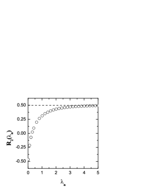
FIG. 1.: Numerical data for the correlator $R_{2}$ versus the scaling parameter $\lambda_{n}=n/l_{\infty}$. The transition from the ballistic to localized regime is shown for for $E=1.5$ and $W=0.1$. The average was done over $10^{4}$ realizations of the disorder. An additional ”window moving” average was performed in order to reduce fluctuations.

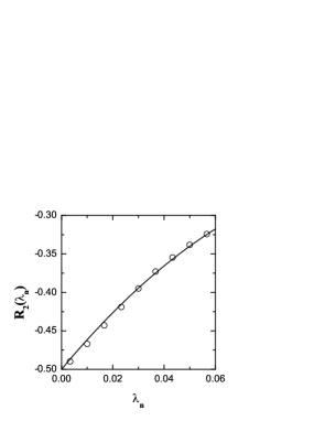
FIG. 2.: Numerical data (open circles) for $R_{2}(\lambda_{n})$ versus Eq.(22) (solid curve) for the same parameters as in Fig.1. and $\lambda_{n}\ll 1$

In order to evaluate analytically the correlator $R_{2}$ in the ballistic regime, we use the approximate map for the angle $\theta_{n}$. It is obtained from Eq.(3) in the limit $|\epsilon_{n}|\ll 1$,

$$\theta_{k+1}=\theta_{k}-\mu+\epsilon_{k}\frac{\sin^{2}\theta_{k}}{\sin\mu}.$$ (21)

Using this recursion, one can express an angle $\theta_{n}$ in terms of the amplitudes $\epsilon_{0},\epsilon_{,}...,\epsilon_{n-1}$ of all the previous kicks for a fixed value of $\mu$. Then the following expression for $R_{2}$ can be obtained [20],

$$R_{2}(\lambda_{n})=-\frac{1}{2}+4\lambda_{n}-16\lambda^{2}_{n}.$$ (22)

In Fig.2 we plot this formula together with numerical data for the ballistic regime, $\lambda_{n}\ll 1$. One can see that there is a complete agreement between numerical and analytical results.

The four-point correlator $S_{4}$, see Eq.(18), can be calculated analytically in a similar way [20],

$$S_{4}(\lambda)=8\lambda^{2}+O\left(\lambda^{3}\right)\;\;.$$ (23)

Substitution of Eqs.(22) and (23) into Eq.(15), gives the following formula for the mean value of $\ln Z_{L}$

$$\left<\ln Z_{L}\right>\approx 4\lambda-8\lambda^{2}+O\left(\lambda^{3}\right)\;\;.$$ (24)

In the same way we calculate the mean value of the second moment,

$$\left<\mbox{ln}^{2}Z_{L}\right> \approx 32\lambda^{2}+O\left(\lambda^{3}\right)\;\;.$$ (25)

Substituting Eqs.(24) and (25) into Eqs.(13) and (14) respectively, we obtain,

$$\left<T_{L}\right>=1-2\lambda+4\lambda^{2}+O\left(\lambda^{3}\right)\;\;,$$ (26)

and

$$\left<T_{L}^{2}\right>=1-4\lambda+16\lambda^{2}+O\left(\lambda^{3}\right)\;\;.$$ (27)

As a result, the variance reads as follows,

$$\text{Var}(T_{L})=\left<T_{L}^{2}\right>-\left<T_{L}\right>^{2}=4\lambda^{2}+O\left(\lambda^{3}\right).$$ (28)

The latter expression for $\text{Var}(T_{L})$ is known in the literature (see, for example, [22]). However, from the analysis of Eqs.(26) and (27) one can obtain a more accurate expression that depends on higher powers of $\lambda$. Indeed, the expansions in (26) and (27) can be considered as asymptotics of the following ”exact” formulas,

$$\left<T_{L}\right>=\frac{1}{1+2\lambda}\,\,\,,$$ (29)

and

$$\left<T_{L}^{2}\right>=\frac{1}{1+4\lambda}\,\,\,.$$ (30)

We have tested these expressions and found that they fit the numerical data much better than Eqs.(26) and (27) [20]. By combining Eq.(29) with (30), one can obtain the following expression for the variance of the transmission coefficient,

$$\text{Var}(T_{L})=\frac{4\lambda^{2}}{(1+4\lambda)(1+2\lambda)^{2}}\,\,\,.$$ (31)

In Fig.3 we compare different approximations for $\text{Var}(T_{L})$ with numerical data. It is clear that Eqs.(29-31) give a very good agreement. Note that the region of validity of the standard expression (28) obtained in the quadratic approximation is very narrow because the numerical coefficients at higher terms ($\lambda^{3},\,\lambda^{4}$, etc) in the expansion of ${\text{Var}}(T_{L})$ grow rapidly.

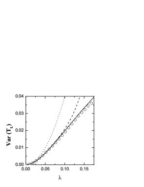
FIG. 3.: Analytical estimates of the mean variance $\text{Var}(T_{L})$ plotted against the numerical data (open circles) for $E=1.5$ and $W=0.1$, with the average over $10^{4}$ realizations of disorder. Dots stand for the standard quadratic approximation (28), dashed lines represent the estimate that takes into account terms up to the sixth power of $\lambda$ in the expansions of $\left<\mbox{ln}Z_{L}\right>$ and $\left<\mbox{ln}^{2}Z_{L}\right>$, namely, $\text{Var}(T_{L})=4\lambda^{2}-32\lambda^{3}+176\lambda^{4}-832\lambda^{5}+3648\lambda^{6}$. The full curve corresponds to our expression (31).

IV Localized regime.

In sufficiently long samples a regime of strong localization, $\lambda=L/l_{\infty}\gg 1$, is realized. Unlike the previous case, now all the trajectories of the classical map (3) move off the origin of the phase space very fast. This means that the radii $r_{L,i=1,2}$ are rapidly growing functions of discrete time $L$. Therefore, in this case $Z_{L}\gg 1$ and it is convenient to represent the transmission coefficient $T_{L}$ in the form,

$$T_{L}=\frac{2}{1+Z_{L}}=\frac{1}{Z_{L}}\frac{2}{1+\frac{1}{Z_{L}}}=\eta_{L}\frac{2}{1+\eta_{L}}.$$ (32)

Here we introduced a small parameter $\eta_{L}=1/Z_{L}\ll 1$ in order to develop a perturbative approach. In the lowest approximation we have,

$$T_{L}=2\,\eta_{L}=\frac{2}{Z_{L}}\,\,.$$ (33)

It is known that in a strongly localized regime the transmission coefficient is exponentially small and reveals very strong fluctuations. For this reason, $T_{L}$ is not a self-averaged quantity, and it is worth to study the logarithm of $T_{L}$. Its mean value is given by

$$\left<\mbox{ln}\,T_{L}\right>=\mbox{ln}\,2-\left<\mbox{ln}Z_{L}\right>,$$ (34)

where the mean value of $\ln Z_{L}$ again can be expressed in terms of the classical trajectories of the map (3),

$$\left<\mbox{ln}Z_{L}\right>=2\lambda-\ln 2+R_{\infty}.$$ (35)

Here the effect of correlations between the phases $\theta_{n}^{(1)}$ and $\theta_{n}^{(2)}$ enters in the last term,

$$R_{\infty}=\left<\mbox{ln}{\left\{1+\exp{\left[\sum_{n=0}^{L-1}A_{n}\left(\sin{2\theta_{n}^{(2)}}-\sin{2\theta_{n}^{(1)}}\right)\right]}\right\}}\right>.$$ (36)

The detailed analysis [20] of this expression shows that, in fact, the term $R_{\infty}$ is independent of the sample length $L$. To justify this we need to take into account that in the limit $\lambda_{n}\rightarrow\infty$ the correlator (20) shown in Fig.1 approaches $1/2$, that is the mean value of $\sin^{2}\theta$. Therefore, the phases $\theta_{0}^{(1)}$ and $\theta_{0}^{(2)}$ fluctuate coherently in such a way that

$$\sin\left(2\theta_{n}^{(2)}\right)-\sin\left(2\theta_{n}^{(1)}\right)\rightarrow 0\,\,\,$$ (37)

for $n\rightarrow\infty$ (this result is analytically proved in [20]).

For this reason the upper limit in the sum in Eq.(36) can be replaced by $L=\infty$. Then the correlation term $R_{\infty}$ becomes $L-$independent. The latter indicates that this term is $l_{\infty}$-independent, as well, due to the scaling dependence of $T_{L}$ on the parameter $\lambda$. Being $\lambda$ independent, the correlation term $R_{\infty}$ is a constant. Unfortunately, we are unable to evaluate this term analytically. The main difficulty is that the strength of the correlations between phases changes along the trajectory, see Fig.1. At the initial stage of evolution when the correlator (20) is different from $1/2$, the two trajectories are neither statistically independent nor coherent. This initial stage gives a contribution, which being small in the localized regime, nevertheless clearly shows that the statistics of $\ln Z_{L}$ and $\ln{T_{L}}$ is not exactly Gaussian (see below).

We evaluated the term $R_{\infty}$ numerically and obtained that the following relation holds with a high accuracy,

$$R_{\infty}-2\ln 2=0\,\,\,.$$ (38)

Substituting Eq.(38) into Eq.(34) we get the standard expression for the mean value of $\ln T_{L}$,

$$\left<\mbox{ln}\,T_{L}\right>=-2\lambda\,.$$ (39)

Since this formula takes into account the correlations along the whole trajectory, it is accurate up to the zero order term with respect to $\lambda$.

In the localized regime the transmission coefficient and its logarithm exhibit strong fluctuations. The approximate distribution function for $\ln{Z_{L}}$ can be easily obtained if we neglect the initial stage of the trajectory and substitute $r_{n}^{(1)}\approx r_{n}^{(2)}$ in Eq.(4). Then, for $\ln{Z_{L}}$ we obtain

$$\ln Z_{L}\approx r_{L}^{2}=\sum\limits_{n=1}^{L}\ln D_{n}^{2}\approx\sum\limits_{n=1}^{L}A_{n}\sin 2\theta_{n}+\Gamma_{2}\,\,\,,$$ (40)

where

$$\Gamma_{2}=\sum\limits_{n=1}^{L}\left(-\frac{1}{2}A_{n}^{2}\sin^{2}2\theta_{n}+A_{n}^{2}\sin^{2}\theta_{n}\right)\,\,\,.$$ (41)

The first term in the last form of Eq.(40) is a sum of $L>>1$ random independent numbers. Therefore, the statistical distribution of $\ln Z_{L}$ is the Gaussian if the quadratic terms $\Gamma_{2}$ are neglected. Thus, we can conclude that the log-norm distribution for the transmission coefficient in the localized regime is obtained in the lowest approximation with weak disorder, and neglecting the difference (37) between phases along the two trajectories.

The parameters of the Gaussian distribution for $\ln Z_{L}$ are calculated from Eq.(40), where the first (linear) term has the zero mean, however, a wide dispersion. The non-zero correction comes from the second (quadratic) term, $\left<\ln Z_{L}\right>=\left<\Sigma_{2}\right>\approx\frac{1}{4}L\left<A_{n}^{2}\right>=2\lambda$. Calculating the second moment of $\ln Z_{L}$ we can neglect the quadratic term in Eq.(40) and get,

$$\left<\ln^{2}Z_{L}\right>\approx 4\lambda+(2\lambda)^{2}\,\,\,.$$ (42)

Then, for the variance of $\ln Z_{L}$ we have,

$$\sigma^{2}\equiv\left<\ln^{2}Z_{L}\right>-\left<\ln Z_{L}\right>^{2}\approx 4\lambda\,,$$ (43)

Now we can write the distribution function for $\ln Z_{L}$,

$${\cal P}\left(\mbox{ln}Z_{L}\right)=\frac{1}{\sqrt{2\pi\sigma^{2}}}\,\exp\left[-\frac{\left(\mbox{ln}Z_{L}-\left<\mbox{ln}Z_{L}\right>\right)^{2}}{2\sigma^{2}}\right]\,\,\,.$$ (44)

In Fig.4 we fit the numerical data obtained for $\lambda=10$ by the Gaussian distribution Eq.(44), using the dispersion $\sigma$ as a fitting parameter. The best fit was obtained for $\sigma^{2}=4\lambda+C_{0}$ with $C_{0}=3.2$, and $\left<\mbox{ln}Z_{L}\right>=2\lambda+\ln 2$. The small correction $C_{0}$ to the dispersion $4\lambda$ originates from the initial stage of the trajectories that is neglected in Eq.(43). At the same time, the center of the distribution (the mean value) is in agreement with Eq.(35) where the calculation is performed exactly.

FIG. 4.: Numerical data (broken curve) for the probability distribution of $\mbox{ln}Z_{L}$ plotted against Eq.(44) (smooth curve). Numerical data were obtained for $E=1.5$, $W=0.1$ and $\lambda=L/l_{\infty}=10$ for $10^{4}$ realizations of the disorder.

It should be noted that if the parameter $\lambda$ is not very big, the numerical histogram for ${\cal P}(\ln Z_{L})$ manifests an asymmetry. The left tail reveals a natural cutoff at $\ln Z_{L}=0$ since $\ln{Z_{L}}$ is a positive function, see Eqs.(7) and (11). This asymmetry is not visible as long as the dispersion $\sigma=2\sqrt{\lambda}$ is much less than the mean value $2\lambda$.

The log-norm distribution Eq.(44) leads to the following mean value for the transmission coefficient [20],

$$\left<T_{L}\right>\approx\left(\frac{\pi}{2}\right)^{\frac{1}{2}}\left(\frac{L}{l_{\infty}}\right)^{-\frac{1}{2}}\exp\left(-\frac{L}{2l_{\infty}}\right)\,\,\,.$$ (45)

This result is slightly different from the exact formula (see, e.g, [21, 22]),

$$\left<T_{L}\right>\approx\left(\frac{\pi}{2}\right)^{\frac{5}{2}}\left(\frac{L}{l_{\infty}}\right)^{-\frac{3}{2}}\exp\left(-\frac{L}{2l_{\infty}}\right)\,\,\,.$$ (46)

Having the same exponential dependence, the approximate expression (45) differs from the exact one by an extra factor $(\pi/2)^{2}\left(L/l_{\infty}\right)^{-1}$. This discrepancy originates from the above-mentioned contribution of the initial stage of evolution that is neglected in the distribution function Eq.(44).

V Conclusions.

We have studied the transport properties of the 1D standard Anderson model with weak random potential, using the Hamiltonian map approach. This approach is based on a reduction of the quantum model to the classical two-dimensional map that describes the dynamics of a linear parametric oscillator with a delta-kick time dependence of its frequency. Amplitudes of the kicks are determined by the site potential of the original quantum model, and the energy of an eigenstate enters into the map as a free parameter.

Some results have been already obtained with the use of this approach in application to both uncorrelated and correlated random potentials [7, 9, 10, 14, 19, 15, 16]. All these studies refer to the properties of the localization length in infinite samples. In contrast to previous results, in this paper we consider a new question about the effectiveness of the Hamiltonian map approach in application to transport properties of finite samples. Specifically, we are interested in the mean values of the transmission coefficient $T_{L}$, its second moment, variance, and the distribution functions.

We performed an analytical treatment for two limit cases of ballistic and strongly localized regimes assuming weakness of the random potential. For the ballistic regime (when $l_{\infty}\gg L$) we were able to derive analytical expressions for the mean values $\left<T_{L}\right>\,,\left<T_{L}^{2}\right>$ and the variance $\left<T_{L}^{2}\right>-\left<T_{L}\right>^{2}$, that are much more accurate that the standard estimates known in the literature. The analysis has revealed a non-trivial role of the correlations between two complimentary classical trajectories that determine the transmission coefficient. Our numerical study confirms the analytical predictions.

For strongly localized regime, $l_{\infty}\ll L$, our main interest was in the mean value of the logarithm of $T_{L}$ and in the distribution function for $\ln T_{L}$. We have found that the leading term for $\left<\ln T_{L}\right>$ can be easily obtained if one neglects the initial stage of the evolution of the complementary classical trajectories. It is also easy to show that the distribution of $\ln T_{L}$ has the Gaussian form. In terms of the classical map, this log-norm distribution results from the central limit theorem applied to the expression for the radius of classical trajectories. Correspondingly, the approach easily reproduces the estimates for the mean value of the second moment of $\ln T_{L}$ and for its variance.

The results of our analysis may find further applications to the problem of the single parameter scaling, as well as in the study of transport properties of 1D random models with long-range correlations in the site potential.

VI Acknowledgments

The authors are very thankful to Luca Tessieri for his valuable comments and fruitful discussions. This research was supported by Consejo Nacional de Ciencia y Tecnología (CONACYT, México) grant 34668-E.

REFERENCES

- [1] E.Abrahams, P.W.Anderson, D.C.Licciardello, and T.V.Ramakrishnan, Phys. Rev. Lett., 42, 673 (1979).
- [2] L.I.Deych, A.A.Lisyansky, and B.L.Alstshuler, Phys. Rev. Lett., 84 2678 (2000); Phys. Rev. B 64, 224202 (2001); L.I.Deych, M.V.Erementchouk, and A.A.Lisyansky, cond-mat/0207269.
- [3] P.W.Anderson, D.J.Thouless, E.Abrahams, and D.S.Fisher, Phys. Rev. B 22, 3519 (1980).
- [4] J.C.Flores, J.Phys. Condens. Matter 1, 8471 (1989); D.H. Dunlap, H-L. Wu, and P.W. Phillips, Phys. Rev. Lett., 65, 88 (1990); P.Phillips and H.-L.Wu, Science 252, 1805 (1991).
- [5] J.S.Denbigh and N.Rivier, J.Phys. C:Solid State Phys. 12, L107 (1979); A.Crisanti, C.Flesia, A.Paquarello, and A.Vulpiani, J.Phys:Condens.Matter 1, 9509 (1989).
- [6] F.A.B.F.de Moura and M.L.Lyra, Phys. Rev. Lett. 81, 3735 (1998); Physica A 266, 465 (1999); F.A.B.F.de Moura, M.D.Continho-Filho, E.P.Raposo, and M.L.Lyra, Phys. Rev. B 66, 014418 (2002).
- [7] F.M. Izrailev and A.A. Krokhin, Phys. Rev. Lett. 82, 4062 (1999); Ann. Phys. (Leipzig) 8, 153 (1999).
- [8] A.A. Krokhin, F.M. Izrailev, U. Kuhl, H.-J. Stöckmann, and S. Ulloa, Physica E 13, 695 (2002).
- [9] A.A. Krokhin and F.M. Izrailev, Comunicaciones Opticas, 1, 16 (2000).
- [10] F.M. Izrailev, A.A. Krokhin, and S.E. Ulloa, Phys. Rev. E., 63, 041102 (2001).
- [11] F.M. Izrailev and N.M. Makarov, Optics Lett. 26, 1604 (2001).
- [12] U. Kuhl, F.M. Izrailev, A.A. Krokhin, and H.-J. Stöckmann, Appl. Phys. Lett. 77, 633 (2000).
- [13] F.M.Izrailev and N.M.Makarov, cond-mat/0209602.
- [14] F.M. Izrailev, T. Kottos and G.P. Tsironis, Phys. Rev. B 52, 3274 (1995).
- [15] F.M. Izrailev, S. Ruffo, and L. Tessieri, J. Phys.: Math. Gen. 31, 5263 (1998).
- [16] L. Tessieri and F.M. Izrailev, Phys. Rev. E., 62, 3090 (2000); Phys. Rev. E., 64, 066120 (2001).
- [17] K.Yu.Bliokh, Zh. Eksp. Teor. Fiz. 121, 14 (2002) [Sov. Phys.-JETP 94, 8 (2002)].
- [18] D.J. Thouless, Phys. Rev. Lett.61, 2141 (1988).
- [19] T. Kottos, G.P. Tsironis and F.M. Izrailev, J. Phys.: Condens. Matter 9, 1777 (1997).
- [20] V. Dossetti-Romero, F.M. Izrailev, and A.A. Krokhin, to be published.
- [21] I.M. Lifshitz, S. Gredeskul, and L. Pastur, Introduction to the Theory of Disordered Systems (Wiley, New York, 1988).
- [22] M.R. Zirnbauer, Phys. Rev. Lett.69, 1584 (1992); A.D. Mirlin, A. Müller-Groeling, and M.R. Zirnbauer, Ann. Phys. 236, 325 (1994); N.M. Makarov, lectures on Spectral and Transport Properties of One-Dimensional Disordered Conductors, [http://www.ifuap.buap.mx/virtual/page_vir.html].