A novel approach to synchronization in coupled excitable systems

Abstract

We consider networks of coupled stochastic oscillators. When coupled we find strong collective oscillations, while each unit remains stochastic. In the limit $N\to\infty$ we derive a system of integro-delay equations and show analytically that the collective oscillations persist in a large region in parameter. For a regular topology with few connections between the oscillators, islands of coherent oscillations are formed, which merge as the amount of topological disorder increases. We link this transition to typical network quantities in the framework of small-world networks.

Collective behavior or synchronization of non-equilibrium systems is one of the main topics in current complex systems research. It can be observed in a variety of different physical, biological and sociological frameworks, such as sub-excitable media, in which noise-induced coherent patterns emerge Zhou , neurons in the brain, where spike patterns synchronize during expectancy or attention EngelFriesSinger , or in an enthusiastic audience which applauds in synchrony after a good performance NedaBarabasi .

Starting from the pioneering work of Winfree Winfree and Kuramoto Kuramoto ; Strogatz2 on coupled phase oscillators, numerous studies have focussed on systems where the dynamics of the single units is deterministic PikovskyBook . Even in systems consisting of coupled chaotic units phase locking may occur Rosenblum . However, many systems are intrinsically stochastic or driven by noise. Numerical investigations show, that synchronization can be found there as well Nikitin ; Kurrer ; Hempel ; Neiman99 , or that it may even be induced by a suitable chosen noise strength PikovskyKurthsCR ; Lindner_CR_SR . To really understand why, and under which conditions synchronization appears in coupled stochastic systems, analytically tractable models are indispensable. There, however, little advancement has been achieved so far.

In this Letter we introduce a system of $N$ coupled discrete stochastic oscillators, each oscillator serving as a prototype of an excitable system. We find large coherent oscillations of the ensemble. In the limit $N\rightarrow\infty$ we show analytically that this coherence is due to a Hopf bifurcation in the dynamics of the ensemble distributions in case of a global coupling. Furthermore, we show numerically, that the synchronization is preserved even if there are only few connections between the oscillators. In contrast to previous investigations Percora ; Kaneko it becomes most pronounced for a large amount of randomness in the topology of the network, which we study in the framework of small world networks WattsStrogatz .

Figure 1: Three state model of an excitable unit. The process $1\to 2$ is Markovian, while the transitions $2\to 3$ and $3\to 1$ are deterministic with a fixed waiting time

We consider a system of $N$ stochastic units. Each unit is a prototypical model of a stochastic excitable oscillator characterized by an attracting fix point $1$ from which it escapes by noise to an excited state $2$. It then performs a long excursion $3$ and finally returns to its rest state $1$ (Fig. 1). The transition $1\rightarrow 2$ is controlled by a rate $\gamma$ which can be expressed as an Arrhenius-like relation Lindner_Fhn . The probability to stay the time $t$ in $1$ is thus given by,

$$w_{1\rightarrow 2}\left(t\right)=\gamma\exp\left(-\gamma t\right)\,,$$ (1)

with mean and standard deviation $1/\gamma$. The transitions $2\to 3$ and $3\to 1$ are deterministic with a peaked waiting time distributions at $\tau_{2}$ and $\tau_{3}$, respectively:

$$w_{2\rightarrow 3}\left(t\right)=\delta(t-\tau_{2})\,,\leavevmode\nobreak\ w_{3\rightarrow 1}\left(t\right)=\delta(t-\tau_{3})\,.$$ (2)

To demonstrate that the dynamics of each individual unit shows typical features of excitable systems we inspect its power spectrum. Setting the output $s(t)=1$ if the unit is in state $3$ at time $t$, and $s(t)=0$, otherwise, the spectrum is then determined employing renewal theory Stratonovich :

$$S(\omega)={\frac{4}{\omega^{2}({1/\gamma}+T)}}{\rm Re}\frac{(1-{{\rm i}\omega/\gamma}-{e^{{\rm i}\omega\tau_{2}}})\left(1-e^{{\rm i}\omega(T-\tau_{2})}\right)}{1-{{\rm i}\omega/\gamma}-e^{{\rm i}\omega T}}\,.$$ (3)

Figure 2: Power spectrum of a single three state unit with $\tau_{2}=0.1$, $\tau_{3}=1.2$ and $1/\gamma=1.0$ (solid line), $1/\gamma=10.0$ (dashed line). For small values of $1/\gamma$ the process is oscillating

where $T=\tau_{2}+\tau_{3}$. The stochasticity of the process can be controlled by varying the amount of time spent in state $1$ compared to $T$. If $1/\gamma\gg T$, the system spends a lot of time in state $1$ and the stochasticity of the first step dominates the dynamics. The spectrum decreases then monotonically until it becomes zero at $\omega_{0}=2\pi/\tau_{3}$. Contrary, for $1/\gamma\ll T$ the process becomes oscillating. (Fig. 2).

To couple the units, we first introduce the dynamic order parameter of the ensemble:

$$f(t)=\frac{1}{N}\sum_{i=1}^{N}s_{i}(t)\,,$$ (4)

with $s_{i}(t)$ denoting the output of unit $i$. A prototypical coupling between the individual oscillators is introduced by letting the rate $\gamma$ functionally depend on the value of $f(t)$ in an inhibitory sigmoidal fashion:

$$\gamma(f(t))\,=\,\gamma_{0}\,\left(1+\Delta\tanh\left[-\frac{f(t)-f^{*}}{2\sigma}\right]\right)\,.$$ (5)

Choosing $\Delta>0$, the transition rate is large for small values and small for large values of $f(t)$. The position and width of the transition is mediated by the parameters $f^{*}$ and $\sigma$. In the following the position $f^{*}$ is kept equal to $0.5$. The inverse of the parameter $\sigma$ can be seen as an effective coupling parameter. If $\sigma\gg 1$, the coupling depends weakly on the value of $f(t)$ and $\gamma$ is approximately equal to $\gamma_{0}$. Contrary, in the case of $\sigma\ll 1$, a sharp transition between the two rates $\gamma_{2/1}=\gamma_{0}(1\pm\Delta)$ occurs if $f(t)$ crosses $f^{*}$. A typical trajectory of $f(t)$ is shown in Fig. 3 for a system consisting of $N=1000$ units. Although each individual unit is governed by the stochastic transition $1\rightarrow 2$, the whole system shows an undamped oscillation, which resembles coherence resonance in coupled excitable Fitz-Hugh-Nagumo units Hempel ; Neiman99 .

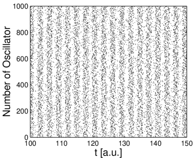
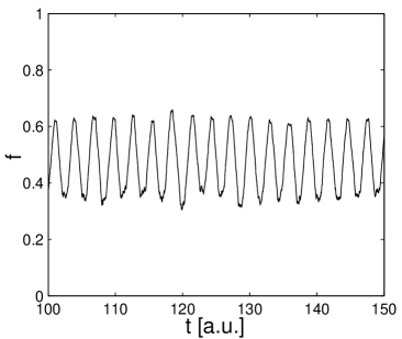
Figure 3: Spike train for a globally coupled network (top) of $N=1000$ oscillators. Each time an oscillator performs a $2\rightarrow 3$ transition a point is plotted. The lower panel shows the dynamic order parameter $f(t)$. In all figures the following parameters were used: $T=2.5$, $\tau_{2}=0.5$, $\gamma_{0}=0.5$, $\Delta=0.6$, $\sigma=10^{-5}$ and $f^{*}=0.5$.

The simplicity and discrete nature of our model allows to derive an analytic condition from an integro-delay equation for the onset of the coherent oscillations. In the limit $N\rightarrow\infty$ the state of the system can be described by the ensemble averaged occupation probabilities $P_{k}(t)$, i.e. the probability that a unit is in state $k$ at time $t$. Following a mean field assumption, we identify the order parameter $f(t)$ with $P_{3}(t)$. The dynamics is then described by the following set of integro-delay equations

$$P_{1}(t) = 1-P_{2}(t)-P_{3}(t)$$

$$P_{2}(t) = \int_{t-\tau_{2}}^{t}\gamma(P_{3}(t^{\prime}))P_{1}(t^{\prime})\,dt^{\prime}$$ (6)

$$P_{3}(t) = \int_{t-T}^{t-\tau_{2}}\gamma(P_{3}(t^{\prime}))P_{1}(t^{\prime})\,dt^{\prime}\,.$$

While the first equation expresses the normalization condition, the second and third account for the balance of probability. The probabilities $P_{2}(t)$ and $P_{3}(t)$ are equal to the time-integrated decay from state $1$ from time $t-\tau_{2}$ up to $t$ and from $t-T$ up to $t-\tau_{2}$, respectively. Similar equations have been investigated before in the framework of delayed differential equations glasslongtin . For a two state rate equation, however, only a resonant-like behavior has been found ohira .

Now we consider the unique stationary fix-point of the nonlinear delay system (A novel approach to synchronization in coupled excitable systems) by setting $P_{k}(t)=P^{*}_{k}$ uniqueFP . This leads to an implicit relation for e.g. $P_{3}^{*}$

$$P_{3}^{*}=\frac{\tau_{3}}{T+1/\gamma\left(P_{3}^{*}\right)}\,,$$ (7)

which is the ratio between the time spent in state $3$ and the mean time for one round trip. Analogous relations may be derived for $P_{1}^{*}$ and $P_{2}^{*}$. To investigate the stability of the single steady state we add small perturbations $P_{k}(t)=P_{k}^{*}+\delta P_{k}(t)$ with $\sum_{k=1}^{3}\delta P_{k}=0$. Using $\delta P_{k}(t)\propto\exp(\lambda t)$ with $\lambda\neq 0$ leads after linearization of Eqs. (6) to the characteristic equation:

$$1+\lambda^{-1}\left\{\gamma(P_{3}^{*})\left(1-e^{-\lambda T}\right)-s\left(e^{-\lambda\tau_{2}}-e^{-\lambda T}\right)\right\}=0.$$ (8)

Here we have introduced $s=\gamma^{\prime}(P_{3}^{*})P_{1}^{*}<0$ and $\gamma^{\prime}(\cdot)$ as the first derivative of $\gamma(\cdot)$.

The solutions of Eq. (8) in $\lambda=\lambda^{\prime}+{\rm i}\lambda^{\prime\prime}$, $\lambda^{\prime},\lambda^{\prime\prime}\in\mathbb{R}$ are complex. A Hopf bifurcation corresponds to values where $\lambda$ crosses the imaginary axis, for which we can derive a condition by setting $\lambda^{\prime}=0$. This gives in parametric dependence on the frequency $\lambda^{\prime\prime}$ at the bifurcation:

$$\gamma(P_{3}^{*})\left(1-\cos(\lambda^{\prime\prime}T)\right)\,-\,s\,\left(\cos(\lambda^{\prime\prime}\tau_{2})-\cos(\lambda^{\prime\prime}T)\right)\,=\,0$$

$$\lambda^{\prime\prime}\,+\,\gamma(P_{3}^{*})\,\sin(\lambda^{\prime\prime}T)\,+\,s\,\left(\sin(\lambda^{\prime\prime}\tau_{2})-\sin(\lambda^{\prime\prime}T)\right)\,=\,0\,.$$

Figs. 4 and 5 shows the region of coherent oscillations in the $\tau_{2}-\sigma$ and $\gamma_{0}-\sigma$ plane, respectively.

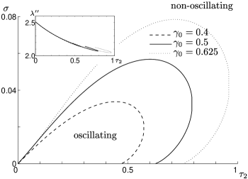
Figure 4: Bifurcation diagram showing the parameter region of coherent oscillations in the $\tau_{2}$-$\sigma$ plane for different values of $\gamma_{0}$. The inset shows the corresponding frequency at the bifurcation, which is nearly independent of $\gamma_{0}$. All other parameters as in Fig. 3

For $\tau_{2}>0$, fixed $\gamma_{0}$ and $\sigma\neq 0$ there is a large region in which the ensemble oscillates. This region grows for increasing values of $\gamma_{0}$. Interestingly, there exist values of $\tau_{2}$ where $\sigma$ has to exceed some finite value to observe the oscillations. When uncoupled, the power spectra of the single units exhibit a maximum at finite frequency for the parameters given by the three curves shown in Fig. 4. However, we would like to stress that coherent oscillations of the ensemble can also be observed if the single uncoupled units are in the non-oscillating regime. The frequency at the bifurcation, as shown in the inset of Fig. 4, which is about $2.2/(2\pi)\approx 0.35$ for $\tau_{2}=0.5$ agrees well with the frequency of the oscillations observed in the numerical simulation (Fig. 3) which is roughly $0.34$.

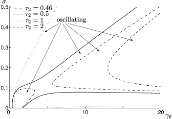
Figure 5: Bifurcation diagram showing the parameter region of coherent oscillations in the $\gamma_{0}$-$\sigma$ plane for different values of $\tau_{2}$. All other parameters as in Fig. 3

The dependence on $\gamma_{0}$ for different values of $\tau_{2}$ is more complex, which we show in Fig. 5. Surprisingly, there are two separated regions of coherent oscillations for small values of $\tau_{2}$ in the parameter plane (dash-dotted lines). This means that a path in the parameter plane in the direction of increasing randomness, i.e.  decreasing $\gamma_{0}$, may cause the oscillations first to vanish and then reappear. Upon increase of $\tau_{2}$ the two regions grow and merge for $\tau_{2}\approx 0.48$ (solid line). The merged region maximizes at $\tau_{2}\approx 1$ (dotted line), further increase of $\tau_{2}$ lets it shrink again (dashed line). In this case, only large values of $\gamma_{0}$ above $\approx 14$ lead to global oscillations.

To complement the globally coupled case, we now investigate diluted networks and the influence of the topology on the onset of coherent oscillations in our system. To study this, we consider a transition from an ordered topology to a random network via small-world networks, which have recently been introduced by Watts and Strogatz WattsStrogatz . The transition is constructed as follows: Starting from a ring with $N$ vertices, each vertex identified as one three state unit, is coupled to its $k$ nearest neighbors with undirected edges. This means, that the transition rate $\gamma_{j}(\cdot)$ of unit $j$ now depends on the local mean field:

$$f_{j}(t)=\frac{1}{k}\sum_{\{i,j\}}s_{i}(t),$$ (9)

$\{i,j\}$ denoting the set of neighbors of vertex $j$. With probability $p$ each edge is then cut and reconnected to a randomly chosen different vertex. In this way the parameter $p$ interpolates between a completely regular ($p=0$) and a random network ($p=1$). Please note that the number of connections is $Nk$ which we require now to be much smaller than the number of all possible connections between vertices, which is $N(N-1)/2$. The small world networks are found for values of $p$ below $\approx 0.1$, where the mean shortest path between two arbitrary nodes drops rapidly, while the cluster index, giving the relative number of common neighbors, is still large (see Fig. 7).

In Fig. 6 we show the dynamics on a completely regular network, i.e. $p=0$.

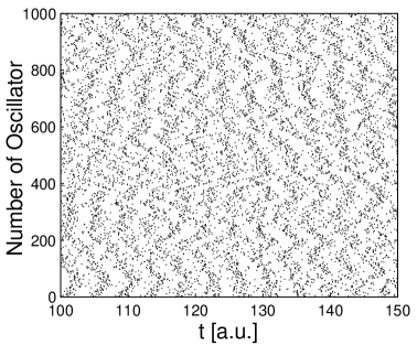
Figure 6: Spike train for a regular network with $p=0$, $N=1000$ and $k=18$. Each time a stochastic unit undergoes a $2\rightarrow 3$ transition a point is plotted. Other parameters are the same as in Fig. 3

.

There, we find small coherent islands, which interchange over time. Since these islands are not in phase, there are no global oscillations. As a measure for the size of the global oscillations, we choose the height of the central peak in the power spectrum of $f(t)$. For increasing randomness, i.e. $p>0$, keeping $k$ fixed, the oscillations become more pronounced and are finally maximized for complete disorder, which can be seen in Fig. 7. The transition to macroscopic oscillations shows a threshold behavior at $p\approx 0.2$. In the inset, both the cluster index and the mean path length are shown. Although there is a steep decrease in the mean path length for already small $p\approx 0.01$, the amplitude of the oscillations only starts to increase, as the cluster index becomes smaller. This means, that in our model, completely random networks synchronize best. For the considered stochastic systems this stands in clear contrast to a previous study of chaotic systems Percora , where it was claimed that the small-world route provides better synchronizability, compared to completely random graphs.

Figure 7: Left axis: Location of the maximum amplitude of the spectrum of the dynamic order parameter $f$ ($+\hskip-7.2pt\times$). Right axis: Cluster index (+) and mean shortest path length ($\times$) in the network.

In conclusion we have presented a system of $N$ discrete stochastic units, which constitutes a generic model of coupled excitable systems. When coupled we observed coherent oscillations. In the limit $N\rightarrow\infty$ the system can be described by a system of integro-delay equations. A stability analysis reveals, that the fixed point of the dynamics becomes unstable under variation of the system parameters. We argue that this mechanism is valid for the finite system as presented by simulations.

We further showed numerically, that the coherent oscillations are preserved if the connectivity is strongly diluted. Starting from a regular network with $k$ nearest neighbor connections ($kN\ll(N-1)N/2$) islands of coherent oscillations with different relative phases coexist. With topological disorder these islands merge and macroscopic oscillations of the whole ensemble can be observed. The transition to global oscillations is connected to the cluster index in the network, which drops considerably on the onset of the oscillations.

The authors thank F. Wolf, M. Timme, M. Zaks and J. Freund for useful discussion. This work has been supported by DFG Sfb-555.

References

- (1) L. Q. Zhou, X. Jia, and Q. Ouyang, Phys. Rev. Lett. 88, 138301 (2002)
- (2) A.K. Engel, P. Fries and W. Singer, Nature Rev. Neurosci. 2, 704 (2001).
- (3) Z. Néda, E. Ravasz, Y. Brechet, T. Vicsek and A.L. Barabási, Nature (London) 403, 849 (2000).
- (4) A.T. Winfree, J. Theo. Biol. 16, 15 (1967); J. Theor. Biol. 28, 327 (1970).
- (5) Y. Kuramoto, in: H. Arakai (Ed.), International Symposium on Mathematica Problems in Theoretical Physics, Vol. 39, Springer, New York, 1975.
- (6) S. H. Strogatz, Physica D 143, 1 (2000)
- (7) A. Pikovsky, M. Rosenblum and J. Kurths, Cambridge Univ. Press (2001)
- (8) V. S. Anishchenko et al., Nonlinear Dynamics of Chaotic and Stochastic Systems (Springer, Berlin-Heidelberg-New York, 2002)
- (9) A. Nikitin, Z. Néda, and T. Vicsek, Phys. Rev. Lett. 87, 024101 (2001).
- (10) C. Kurrer and K. Schulten, Phys. Rev. E 51, 6213 (1995).
- (11) H. Hempel, L. Schimansky-Geier, and J. Garcia-Ojalvo Phys. Rev. Lett. 82, 3713 (1999).
- (12) A. Neiman, L. Schimansky-Geier, A. Cornell-Bell, and F. Moss Phys. Rev. Lett. 83, 4896 (1999).
- (13) A.S. Pikovsky, J. Kurths, Phys. Rev. Lett. 78, 775 (1997);
- (14) B. Lindner and L. Schimansky-Geier, Phys. Rev E 61, 6103 (2000).
- (15) M. Barahona and L. M. Pecora, Phys. Rev. Lett. 89, 054101 (2002)
- (16) J. Ito and K. Kaneko Phys. Rev. Lett. 88, 028701 (2002)
- (17) D.J. Watts and S.H. Strogatz, Nature (London) 393, 440 (1998).
- (18) B. Lindner and L. Schimansky-Geier, Phys. Rev. E 60 , 7270 (1999).
- (19) R. L. Stratonovich, Topics in the Theory of Random Noise I (Gordon and Breach, 1962) p. 175.
- (20) M. C. Mackey and L. Glass, Science 197, 287 (1977);J. Milton, A. Longtin, A. Beuter, M.C. Mackey and L. Glass, J. Theor. Biol. 138, 129 (1989)
- (21) T. Ohira and Y. Sato, Phys. Rev. Lett. 82, 2811 (1999)
- (22) The uniqueness of the fix point is due to the chosen coupling function in Eq. (5), which leads to only one solution of Eq. (7).