Correlation effects of carbon nanotubes at boundaries:
Spin polarization induced by zero-energy boundary states

Abstract

When a carbon nanotube is truncated with a certain type of edges, boundary states localized near the edges appear at the Fermi level. Starting from lattice models, low-energy effective theories are constructed which describe electron correlation effects on the boundary states. We then focus on a thin metallic carbon nanotube which supports one or two boundary states and discuss physical consequences of the interaction between the boundary states and bulk collective excitations. By the renormalization group analyses together with the open boundary bosonization, we show that the repulsive bulk interactions suppress the charge fluctuations at boundaries and assist the spin polarization.

I Introduction

A single-wall carbon nanotube (CNT) is a fascinating quasi-one-dimensional (quasi-1D) nano-scale material, which is a graphite sheet wrapped into a cylindrical form. Its electronic structure is basically well described by a one-electron tight-binding model with a single $\pi$ orbital per atom. Depending on its geometrical shape, a large variety of electronic structures are realized. Especially, it can be either a metal or a semiconductor depending on how the graphite sheet is wrapped. hamada92 ; saito92 ; mintmire92 The way of wrapping is specified by a chiral vector $(N,M),N,M\in\mathbb{Z}$. When $N-M\equiv 0\mod 3$ is satisfied, a CNT is metallic, while it is gapped otherwise.

An interesting consequence of its rich electronic band structure is the existence of the boundary states when the system possesses boundaries. For a CNT with zigzag or bearded edges, there appear states localized at the boundaries for specific values of the wave number along the boundaries. fujita96 It is a hallmark of the phase degree of freedom specific to quantum mechanical systems. ryu02 The existence of such boundary states raises an interesting question as to what kind of physical consequences they lead. For example, the electronic and magnetic properties of nanographite in magnetic field wakabayashi99 or electronic transport through nanographite ribbon junctions wakabayashi00 ; wakabayashi01 were theoretically investigated. Furthermore, in the presence of electron-electron or electron-phonon interactions, the boundary states might trigger an instability as they form a flatband and a sharp peak in density of states at the Fermi energy for a 2D sheet geometry. Indeed, spin polarization induced by the boundary states fujita96 ; wakabayashi98 ; okada01 ; hikihara02 ; nakada98 , or coupling with lattice distortions fujita97 ; ryu02 has been studied for a graphite sheet by several authors. The effects of 1D low-lying excitations localized at the boundaries was also discussed for ribbon geometry. lee02

The effects of bulk electron correlations have been extensively investigated for metallic CNT’s without boundaries. egger97 ; egger98 ; yoshioka99 ; odintsov99 ; krotov97 ; balents97 ; lin98 ; kane97 It is claimed that the most important forward scattering part of the Coulomb interaction is well accounted for by the Tomonaga-Luttinger (TL) liquid picture kane97 , where low-lying excitations are not of Fermi liquid type, but bosonic collective excitations. Behaviors specific to TL liquid, such as a characteristic temperature dependence of conductance, have been indeed observed in recent experiments. bockrath99 In TL liquid, boundary critical phenomena are known to be drastically different from the conventional Fermi liquid case when the system possesses boundaries. kane92 ; egger92 ; furusaki93 ; wang94 ; fabrizio95 Then, we expect to see interesting phenomena for a thin metallic CNT with boundaries. The anomalous boundary physics in a metallic CNT within the TL liquid picture such as tunneling density of states egger98 , Freidel oscillation yoshioka02 , or local density of states yoshioka02-2 has been investigated previously, but without boundary states.

The purpose of the present paper is to discuss electron correlation effects for CNT’s with edges that supports boundary states. We consider $(N,-N)$ CNT’s with zigzag and bearded edges, for which boundary states appear at the Fermi level for some values of the wave number along the edges. Starting from lattice models with the Coulomb or the Hubbard interaction, we first establish low-energy effective theories that describe correlation effects at boundaries. We then focus on a thin metallic CNT, where the boundary states interact with the collective bulk excitations. By the renormalization group (RG) analyses together with the open boundary bosonization, we discuss the cases where one or two boundary states exist.

For the case of two boundary states, we are especially interested in whether or not the boundary states exhibit spin polarization in the presence of gapless bulk excitations. The possibility of spin polarization was previously discussed for 2D geometry, i.e., in the limit of the infinite tube radius $N\to+\infty$, by mean field theoryfujita96 or density-functional theory with local spin density approximation (LSDA) okada01 . However, these treatments of electron correlations can overestimate the magnetic instability. Also, when the system is wrapped into a 1D cylinder, one needs further justification. A density matrix renormalization (DMRG) study was also performed hikihara02 which reports spin polarization at boundaries, but only for a semi-conducting CNT. When the bulk part of the system is gapless, it is not clear if the boundary states show spin polarization since the total spin (and charge) carried by the boundary states can dissipate into a bulk part of the system through the electron interactions between boundary states and bulk gapless collective modes.

The paper is organized as follows: section II is devoted to a construction of low-energy effective theories which account for zero-energy boundary states. We recall some known facts on boundary states in section II.1, and the Coulomb or the Hubbard interaction is projected to the low-energy sector of the Hilbert space spanned by the boundary states and gapless bulk modes in section II.2. In section II.3, we perform open boundary bosonization to account for the bulk repulsive interactions and discuss its consequences on boundary physics. Finally, we present RG analyses for the case with one boundary states (section III) and with two boundary states (section IV). We conclude in section V.

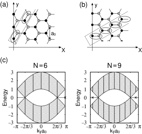
Figure 1: A $(N,-N)$ CNT with (a) zigzag and (b) bearded edges. Two-dimensional graphite sheets are wrapped around the $x$ axis. The ovals indicate how to form a spinor $\bm{c}=\ ^{t}(c_{\bullet},c_{\circ})$, and dotted squares show a choice of unit cell for each types of edges. (c) Energy spectra for a $(N,-N)$ CNT with zigzag edges for $N=6,9$. ($t=1$) Shaded regions represent bulk energy spectra for $N\rightarrow\infty$. Allowed wave numbers along the boundaries for $N=6,9$ are shown by vertical lines. Boundary states are denoted by $\times$.

II Zero energy boundary states and interactions

II.1 Zero energy boundary states

II.1.1 Zigzag edges

Let us first consider a $(N,-N)$ CNT with zigzag edges. Our starting point is the single particle tight-binding Hamiltonian defined on the honeycomb lattice [Fig. 1(a)]:

$$H_{\hbox{\tiny{kin}}} = \sum_{i,j}\Big{[}\bm{c}^{\dagger}(i,j)\,T_{-}\,\bm{c}(i,j+1)+h.c.$$ (1)

$$+\bm{c}^{\dagger}(i,j)\,T_{+}\,\bm{c}(i-1,j+1)+h.c.$$

$$+\bm{c}^{\dagger}(i,j)\,T_{0}\,\bm{c}(i,j)\Big{]},$$

where $\bm{c}=\ ^{t}(c_{\bullet},c_{\circ})$, is a spinor made of electron annihilation operators $c_{\bullet,\circ}$ defined on different sublattices $\bullet,\circ$. Coordinates of the spinors are labeled by the unit cell to which they belong and the location within the unit cell. Unit cells are chosen so as to be compatible with the shape of the edges, and are labeled by their $y$ coordinate $y=ja_{0}$, $j=1,\cdots,N_{y}$, where $N_{y}=N$ is the total number of sites along the $y$ axis and $a_{0}$ the lattice constant. Spinors are located at $X=\sqrt{3}a_{0}i$, $i=1,\cdots,N_{X}$ within a unit cell with $N_{X}$ being the total number of sites along the $X$ axis. Hopping matrix elements for the zigzag case are given by $T_{+}=(-t)\left[\begin{array}[]{cc}0&1\\ 0&0\end{array}\right],$ $T_{-}=(-t)\left[\begin{array}[]{cc}0&0\\ 1&0\end{array}\right],$ and $T_{0}=(-t)\left[\begin{array}[]{cc}0&1\\ 1&0\end{array}\right],$ where $t$ is the hopping integral. As specified by the chiral vector, the periodic boundary condition is imposed along the edges, which renders the wave numbers along the edges quantized, $k_{y}a_{0}=2m\pi/N_{y},m\in\mathbb{Z}$. The band structure is then composed of a set of 1D modes, each of which is characterized by the wave number. Performing a Fourier transformation along the $y$ axis as $\bm{c}(i,j)=1/\sqrt{N_{y}}\sum_{k_{y}}e^{\mathrm{i}k_{y}y}\bm{c}_{k_{y}}(i)$, $H_{\hbox{\tiny{kin}}}$ is decomposed as $H_{\hbox{\tiny{kin}}}=\sum_{k_{y}}H(k_{y})$,

$$H(k_{y}) = \sum_{i=1}^{N_{X}}\Big{[}{\bm{c}}_{k_{y}}^{\dagger}(i)\,V_{X}\,{\bm{c}}_{k_{y}}^{\vphantom{\dagger}}(i+1)+h.c.$$ (2)

$$+{\bm{c}}^{\dagger}_{k_{y}}(i)\,V_{0}\,{\bf c}_{k_{y}}^{\vphantom{\dagger}}(i)\Big{]},$$

where $V_{X}=T_{-}e^{-\mathrm{i}k_{y}a_{0}}$ and $V_{0}=T_{0}+T_{-}e^{+\mathrm{i}k_{y}a_{0}}+T_{+}e^{-\mathrm{i}k_{y}a_{0}}$. This 1D Hamiltonian can be seen as a 1D chain with alternating hoppings.lin98 As for bulk electron states, the energy spectrum is gapless for two values of $k_{y}$, $k_{y}a_{0}=\pm k_{0}a_{0}=\pm 2\pi/3$, whereas it is gapped for other $k_{y}$. This is best seen by performing a gauge transformation $c_{\bullet}(i)\to(-)^{i}e^{+\mathrm{i}k_{y}a_{0}/4}c_{\bullet}(i)$, $c_{\circ}(i)\to(-)^{i}e^{-\mathrm{i}k_{y}a_{0}/4}c_{\circ}(i)$, which transforms the Hamiltonian as $V_{X}\to(-e^{-\mathrm{i}\frac{3}{2}k_{y}a_{0}})T_{-}$ and $V_{0}\to 2\cos(k_{y}a_{0}/2)T_{0}$. Then, the alternation can be completely removed for $k_{y}=\pm k_{0}$, where the Hamiltonian is reduced to $H(\pm k_{0})=-t\sum_{l=1}^{N_{x}}\big{[}c^{\dagger}_{\pm,l}c_{\pm,l+1}+h.c.\big{]}$ by defining $c_{\pm k_{0},\bullet}(i)=:c_{\pm,l=2i-1}$, $c_{\pm k_{0},\circ}(i)=:c_{\pm,l=2i}$, and $2N_{X}=:N_{x}$.

When truncated with edges, the above one-parameter family of Hamiltonians supports zero-energy boundary states for some specific values of $k_{y}$, fujita96 ; ryu02 as a manifestation of a nontrivial bulk band structure. For zigzag edges, they appear for $-\pi<k_{y}a_{0}<-2\pi/3,+2\pi/3<k_{y}a_{0}<+\pi$, within a bulk energy gap at the Fermi energy. The localization length of the boundary states continuously increases as we vary $k_{y}a_{0}$ from $+\pi(-\pi)$ to $+2\pi/3(-2\pi/3)$. For $k_{y}a_{0}=\pm\pi$, the boundary states is completely localized at the boundaries $i=1$ and $N_{X}$, while the localization length for $k_{y}a_{0}=\pm 2\pi/3$ is infinite, at which the branch of the localized boundary states continuously merges with the extended bulk states. If we explicitly construct wave functions for the boundary states, they are given by

$$f_{k_{y},\bullet}(i)\propto\big{(}-2e^{\mathrm{i}3k_{y}a_{0}/2}\cos k_{y}a_{0}/2\big{)}^{i-1},\quad f_{k_{y},\circ}(i)=0$$

(3)

($-\pi<k_{y}a_{0}<-2\pi/3,+2\pi/3<k_{y}a_{0}<+\pi$), after the gauge transformation.

II.1.2 Bearded edges

We turn to a CNT with bearded edges. Atomic configurations realizing bearded edges for $\pi$ electrons were recently proposed based on an ab initio calculation. kusakabe02 We choose a different unit cell from that for the zigzag case as indicated in Fig. 1(b). ($X$ is now equal to $2\sqrt{3}a_{0}i$, $i=1,\cdots,N_{X}$.) We obtain a set of Hamiltonian parametrized by $k_{y}$ as in the zigzag case with the hopping matrices $V_{X}$ and $V_{0}$ being given by $V_{X}=T_{-}+T_{-}e^{-\mathrm{i}k_{y}a_{0}}$, and $V_{0}=T_{0}$. Again, the bulk energy spectrum is gapless for $k_{y}=\pm k_{0}$, for which the Hamiltonian can be transformed to a simple form $H(\pm k_{0})=-t\sum_{l=1}^{N_{x}}\big{[}c^{\dagger}_{\pm,l}c_{\pm,l+1}+h.c.\big{]}$ by a gauge transformation $c_{\bullet}(i)\to e^{+\mathrm{i}k_{y}a_{0}i/2}c_{\bullet}(i)$, $c_{\circ}(i)\to e^{+\mathrm{i}k_{y}a_{0}i/2}c_{\circ}(i)$. On the other hand, boundary states appear for different values of $k_{y}$ from the zigzag case, $-2\pi/3<k_{y}a_{0}<+2\pi/3$. The wave function of the boundary states can be explicitly constructed as

$$f_{k_{y},\bullet}(i)\propto\big{(}-2\cos k_{y}a_{0}/2\big{)}^{-(i-1)},\quad f_{k_{y},\circ}(i)=0$$ (4)

($-2\pi/3<k_{y}a_{0}<+2\pi/3$), after the gauge transformations.

II.2 Interactions

As the boundary states with different $k_{y}$ are all degenerate at the Fermi energy, electron interactions have pronounced effects. In what follows, we will construct low-energy effective theories describing correlation effects on the boundary states. The interacting part of the Hamiltonian is written as

$$H_{\hbox{\tiny{int}}} = \frac{1}{2}\sum_{RR^{\prime};pp^{\prime};ss^{\prime}}V_{RR^{\prime};pp^{\prime};ss^{\prime}}$$ (5)

$$\times c_{ps}^{\dagger}(R)c_{p^{\prime}s^{\prime}}^{\dagger}(R^{\prime})c_{p^{\prime}s^{\prime}}(R^{\prime})c_{ps}(R),$$

where $R=(i,j)$ runs over the lattice cites in the tight-binding model, $p=\bullet/\circ$ represents a sublattice, and $s=\uparrow/\downarrow$ is a spin index. As for $V_{RR^{\prime};pp^{\prime};ss^{\prime}}$, we take either the Hubbard interaction

$$V_{RR^{\prime};pp^{\prime};ss^{\prime}}=U\delta_{RR^{\prime}}\delta_{pp^{\prime}}\delta_{s,-s^{\prime}}$$ (6)

or the unscreened Coulomb interaction

$$V_{RR^{\prime};pp^{\prime};ss^{\prime}}=\frac{e^{2}/\kappa}{\sqrt{(x_{p}-x^{\prime}_{p^{\prime}})^{2}+4R^{2}\sin^{2}\left(\frac{y-y^{\prime}}{2R}\right)+r_{z}^{2}}},$$

where $\kappa$ is an effective dielectric constant of the system, $x_{\bullet}=X$, $x_{\circ}=X+\sqrt{3}a_{0}/2$ (zigzag), $\sqrt{3}a_{0}$ (bearded), $R$ is the tube radius, and $r_{z}\sim a_{0}$ characterizes the radius of $p_{z}$ orbital, serving as a short-distance cutoff. In Ref. egger97, , $\kappa$ is estimated to $\sim 1.4$, while $r_{z}$ is determined to be $0.526\times a_{0}$ in Ref. odintsov99, , from the requirement that the on-site interaction in the original tight-binding model corresponds to the difference between the ionization potential and electron affinity of $sp^{2}$ hybridized carbon. Since the Coulomb interaction is unscreened in CNT’s, the Hubbard interaction is less realistic. However, as we will see, their differences are small for the correlation effects at boundaries, due to the special properties of the boundary states, although the long-range nature of the Coulomb interaction has fundamental effects for the bulk electron states.

Focusing on a low-energy sector, we construct a effective theory with boundary states at zero energy. When a CNT is metallic, two 1D gapless modes are also included, while we drop all the operators belonging to gapped bands:

$$\bm{c}(i,j) = \frac{1}{\sqrt{N_{y}}}\sum_{k_{y}}e^{\mathrm{i}k_{y}y}\bm{c}_{k_{y}}(i)$$

$$\longrightarrow \frac{1}{\sqrt{N_{y}}}\sum_{\alpha=\pm}e^{\mathrm{i}\alpha k_{0}y}\bm{c}_{\alpha}(i)+\frac{1}{\sqrt{N_{y}}}\bm{b}(i,j),$$

where $\bm{c}_{\pm}(i):=\bm{c}_{\pm k_{0}}(i)$, $\bm{b}$ is a linear combination of boundary states, $\bm{b}(i,j)=\sum_{k_{y}}^{\prime}e^{\mathrm{i}k_{y}y}\bm{f}_{k_{y}}(i)\,e_{k_{y}}$, with $\bm{f}_{k_{y}}(i)$ being an eigen wave function localized at boundaries, $e_{k_{y}}^{\dagger}$ and $e_{k_{y}}^{\vphantom{\dagger}}$ are creation and annihilation operators for a boundary state, and $\sum^{\prime}$ means the summation is restricted to the wave numbers for which a boundary state appears. We project the interaction $H_{\hbox{\tiny{int}}}$ into the reduced Hilbert space spanned by the two gapless modes $\bm{c}_{\pm}^{\dagger}$, $\bm{c}_{\pm}$ and the boundary states $e_{k_{y}}^{\dagger}$, $e_{k_{y}}$. Substituting Eq. (LABEL:dropping_operators), $H_{\hbox{\tiny{int}}}$ is decomposed into a number of terms, each of which is a four-fermion interaction made of either $\bm{c}_{\pm}^{\dagger}$, $\bm{c}_{\pm}$, $e_{k_{y}}^{\dagger}$, or $e_{k_{y}}$. However, not all of them give rise to a contribution due to the momentum conservation along the edges. For example, a four-fermion interaction composed of three bulk electrons and one edge electron (e.g., $c_{+s}^{\dagger}c_{-s^{\prime}}^{\dagger}c_{-s^{\prime}}^{\vphantom{\prime}}b_{s^{\prime}}^{\vphantom{\prime}}$) does not appear for the zigzag cases since the momentum carried by the bulk electron is either $+2\pi/3$ or $-2\pi/3$, while that carried by the edge electrons is never equal to $\pm 2\pi/3$, and hence a momentum mismatch occurs. It should be also noted that boundary states are nonvanishing only on one of sublattices $p=\bullet$ as seen from Eqs. (3) and (4). Due to this special property of boundary states and also since the boundary states are localized at boundaries, the Coulomb interaction and the Hubbard interaction are not quite different. So we restricted ourselves to the Hubbard interaction for a while as it is simpler. We write the projected interaction as $H_{\hbox{\tiny{int}}}\rightarrow H_{\hbox{\tiny{int}}}^{\hbox{\tiny{bulk}}}+H_{\hbox{\tiny{int}}}^{\hbox{\tiny{edge}}}$, where $H_{\hbox{\tiny{int}}}^{\hbox{\tiny{bulk}}}$ is solely composed of bulk electron operators, while $H_{\hbox{\tiny{int}}}^{\hbox{\tiny{edge}}}$ includes boundary states. We further decompose $H_{\hbox{\tiny{int}}}^{\hbox{\tiny{edge}}}$ as $H_{\hbox{\tiny{int}}}^{\hbox{\tiny{edge}}}=H_{\hbox{\tiny{int}}}^{\hbox{\tiny{edge4}}}+H_{\hbox{\tiny{int}}}^{\hbox{\tiny{edge3}}}+H_{\hbox{\tiny{int}}}^{\hbox{\tiny{edge2}}}+H_{\hbox{\tiny{int}}}^{\hbox{\tiny{edge1}}}$. Firs, $H_{\hbox{\tiny{int}}}^{\hbox{\tiny{edge4}}}$ consists solely of boundary states,

$$H_{\hbox{\tiny{int}}}^{\hbox{\tiny{edge4}}} = \frac{U}{N_{y}}\sum_{k_{1},k_{2},k_{3},k_{4}}^{\prime}\delta(-k_{1}+k_{2}-k_{3}+k_{4})$$

$$\times e_{k_{1}\uparrow}^{\dagger}e_{k_{2}\uparrow}^{\vphantom{\dagger}}e_{k_{3}\downarrow}^{\dagger}e_{k_{4}\downarrow}^{\vphantom{\dagger}}\sum_{i}f_{k_{1}}^{*}(i)f_{k_{2}}^{\vphantom{*}}(i)f^{*}_{k_{3}}(i)f_{k_{4}}^{\vphantom{*}}(i),$$

where we simply wrote $f_{k,p=\bullet}$ as $f_{k}$ and $\delta(k)$ is a lattice delta function; i.e., $\delta(k)$ is equal to unity only when $k$ is integral multiple of $2\pi$, while it is vanishing otherwise. When a CNT is insulating, it is enough to consider only $H_{\hbox{\tiny{int}}}^{\hbox{\tiny{edge4}}}$ for boundary physics. Then, the problem is reduced to how the degeneracy between the boundary states with quenched kinetic energy is lifted by $H_{\hbox{\tiny{int}}}^{\hbox{\tiny{edge4}}}$, as in the flatband magnetism or the fractional quantum Hall effect. Note also that the strength of the Hubbard interaction is reduced by the factor $1/N_{y}$, as the wave functions of the boundary states are extended over the circumference of the tube.

The part composed of two edge operators $H_{\hbox{\tiny{int}}}^{\hbox{\tiny{edge2}}}$ is given by

$$H_{\hbox{\tiny{int}}}^{\hbox{\tiny{edge2}}} = \frac{U}{N_{y}}\sum_{i}\Big{[}-2\tilde{J}^{z}\tilde{S}^{z}-\tilde{J}^{+}\tilde{S}^{-}-\tilde{S}^{+}\tilde{J}^{-}$$ (10)

$$+\frac{1}{2}\tilde{\rho}^{\vphantom{\dagger}}\tilde{\rho}_{e}^{\vphantom{\dagger}}+\tilde{\Delta}^{\dagger}\tilde{\Delta}_{e}^{\vphantom{\dagger}}+\tilde{\Delta}_{e}^{\dagger}\tilde{\Delta}^{\vphantom{\dagger}}\Big{]},$$

where

$$\tilde{\bm{J}}=\sum_{\alpha,ss^{\prime}}c_{\alpha s}^{\dagger}\frac{\bm{\sigma}_{ss^{\prime}}}{2}c_{\alpha s^{\prime}},\quad\tilde{\bm{S}}=\sum_{k_{y},ss^{\prime}}^{\prime}|f_{k_{y}}|^{2}e^{\dagger}_{k_{y}s}\frac{\bm{\sigma}_{ss^{\prime}}}{2}e_{k_{y}s^{\prime}},$$

$$\tilde{\rho}=\sum_{\alpha,s}c_{\alpha s}^{\dagger}c_{\alpha s},\qquad\tilde{\rho}_{e}=\sum_{k_{y},s}^{\prime}|f_{k_{y}}|^{2}e^{\dagger}_{k_{y}s}e_{k_{y}s},$$

$$\tilde{\Delta}=\Big{[}c_{+\downarrow}c_{-\uparrow}+c_{-\downarrow}c_{+\uparrow}\Big{]},\quad\tilde{\Delta}_{e}=\sum_{k_{y}}^{\prime}f_{k_{y}}^{2}e_{k_{y}\uparrow}e_{-k_{y}\downarrow}.$$

(11)

We omit sublattice indices and simply write $c_{\pm}=c_{\pm\bullet}$, $b=b_{\bullet}$ henceforth, since $p=\circ$ does not appear. Finally, $H_{\hbox{\tiny{int}}}^{\hbox{\tiny{edge1}}}$ and $H_{\hbox{\tiny{int}}}^{\hbox{\tiny{edge3}}}$ are given by

$$H_{\hbox{\tiny{int}}}^{\hbox{\tiny{edge1}}} = \frac{U}{N_{y}^{2}}\sum_{i,j}\Big{[}c^{\dagger}_{+\uparrow}c^{\vphantom{\dagger}}_{-\uparrow}\left(c^{\dagger}_{+\downarrow}b^{\vphantom{\dagger}}_{-\downarrow}+b^{\dagger}_{\downarrow}c^{\vphantom{\dagger}}_{+\downarrow}\right)+h.c.$$

$$+\left(c^{\dagger}_{+\uparrow}b^{\vphantom{\dagger}}_{-\uparrow}+b^{\dagger}_{\uparrow}c^{\vphantom{\dagger}}_{+\uparrow}\right)c^{\dagger}_{+\downarrow}c^{\vphantom{\dagger}}_{-\downarrow}+h.c.\Big{]},$$

$$H_{\hbox{\tiny{int}}}^{\hbox{\tiny{edge3}}} = \frac{U}{N_{y}^{2}}\sum_{i,j}\Big{[}b^{\dagger}_{\uparrow}b^{\vphantom{\dagger}}_{\uparrow}\big{(}c_{-\downarrow}^{\dagger}b_{\downarrow}^{\vphantom{\dagger}}+b^{\dagger}_{\downarrow}c_{+\downarrow}^{\vphantom{\dagger}}\big{)}+h.c.$$ (12)

$$+\big{(}c_{-\uparrow}^{\dagger}b_{\uparrow}^{\vphantom{\dagger}}+b^{\dagger}_{\uparrow}c_{+\uparrow}^{\vphantom{\dagger}}\big{)}b^{\dagger}_{\downarrow}b_{\downarrow}^{\vphantom{\dagger}}+h.c.\Big{]}.$$

As commented above, $H_{\hbox{\tiny{int}}}^{\hbox{\tiny{edge1}}}$ does not appear for the zigzag cases due to a momentum mis-match. Furthermore, for a thin CNT with zigzag edges, $H_{\hbox{\tiny{int}}}^{\hbox{\tiny{edge3}}}$ is also vanishing and hence the effective Hamiltonian is simplified.

The bulk part of a metallic CNT is described by a simple tight-binding Hamiltonian $H(\pm k_{0})=-t\sum_{l=1}^{N_{x}}\big{[}c_{\pm,l}^{\dagger}c_{\pm,l+1}+h.c.\big{]}$ after the gauge transformation. In describing the gapless excitations, we replace lattice fermion operators $c_{\pm,l}$by slowly varying continuum operators $\psi_{L/R,\pm}(x)$ as

$$c_{\pm,l}\sim\sqrt{a_{x}}\Big{[}e^{+\mathrm{i}k_{F}x}\psi_{L,\pm}(x)+e^{-\mathrm{i}k_{F}x}\psi_{R,\pm}(x)\Big{]},$$ (13)

where $a_{x}:=\sqrt{3}a_{0}/2$, and $x:=2X$. Due to the open boundary conditions, however, the left and right movers are not independent. They satisfy a constraint

$$\psi_{R,\pm}(x)=-\psi_{L,\pm}(-x),$$ (14)

which allows us to concentrate on only the left-moving sector, say. Focusing on the two gapless modes, the kinetic part of the system is written by the slowly varying variables as

$$H_{\hbox{\tiny{kin}}}=v_{F}\sum_{\alpha,s}\int_{-L}^{+L}dx\,\psi^{\dagger}_{L\alpha s}\mathrm{i}\partial_{x}\psi_{L\alpha s},$$ (15)

where $L=N_{x}a_{x}$ and $v_{F}=\sqrt{3}ta_{0}/2$ is the Fermi velocity. Here, the original system defined for $x\in[0,+L]$ is extended to $x\in[-L,+L]$ by the constraint, Eq. (14).

Upon taking continuum limit, we are also allowed to set $X=x=0$ for the interactions that include boundary states with some renormalizations of couplings, since edge modes are exponentially localized at the boundary. The lattice fermion operators at the boundary are replaced with the left moving continuum field as

$$c_{\pm,l=1} \rightarrow \sqrt{a_{x}}\Big{[}e^{+\mathrm{i}k_{F}a_{x}}\psi_{L,\pm}(a_{x})+e^{-\mathrm{i}k_{F}a_{x}}\psi_{R,\pm}(a_{x})\Big{]}$$ (16)

$$\sim \sqrt{a_{x}}\,2\mathrm{i}\sin(k_{F}a_{x})\,\psi_{L,\pm}(0).$$

Correspondingly, operators made of lattice fermions $\tilde{\bm{J}},\tilde{\rho},\tilde{\Delta}^{\dagger},\tilde{\Delta}$ appearing in $H^{\hbox{\tiny{edge2}}}_{\hbox{\tiny{int}}}$ are replaced with continuum counterparts as

$$\bm{J}=\sum_{\alpha,ss^{\prime}}\psi_{L\alpha s}^{\dagger}\frac{\bm{\sigma}_{ss^{\prime}}}{2}\psi_{L\alpha s^{\prime}},\quad\rho=\sum_{\alpha,s}\psi_{L\alpha s}^{\dagger}\psi_{L\alpha s},$$

$$\Delta=\Big{[}\psi_{L+\downarrow}\psi_{L-\uparrow}+\psi_{L-\downarrow}\psi_{L+\uparrow}\Big{]},$$ (17)

with suitable renormalizations for couplings. At this level, also, differences between the Hubbard and the Coulomb interaction are irrelevant, since we keep the same terms for the both types of interactions.

II.3 Effects of the bulk interactions: Open boundary bosonization

Although we are interested in physics at boundaries, effects of electron correlation in the bulk regime $H_{\hbox{\tiny{int}}}^{\hbox{\tiny{bulk}}}$ should also be taken into account, since the bulk interaction is known to affect the scaling dimension of operators inserted at a boundary in 1D correlated systems. The bulk interaction is well incorporated by the bosonization technique for 1D systems. Following Ref. fabrizio95, , we bosonize the theory with open boundary condition. Open boundary bosonization was previously used to discuss the correlation effects of armchair CNTs with boundaries, where there are no boundary states though. egger98 ; yoshioka02 ; yoshioka02-2

Upon bosonization, electron operators are expressed in terms of scalar bosonic operators as

$$\psi_{\alpha s}(x)\equiv\frac{1}{\sqrt{2\pi a_{x}}}\eta_{\alpha s}:e^{+\mathrm{i}\sqrt{4\pi}\varphi_{\alpha s}}:(x),$$ (18)

where $\eta_{\alpha s}$ is a Klein factor, and $:\cdots:$ denotes normal ordering. [Since it is enough to focus on the holomorphic sector, we simply write $\psi_{L\alpha s}(x)=\psi_{\alpha s}(x)$, $\varphi_{L\alpha s}(x)=\varphi_{\alpha s}(x)$, etc., henceforth.] For convenience, it is better to introduce a new basis $\left\{\varphi_{\rho,\pm},\varphi_{\sigma,\pm}\right\}$ rather than $\varphi_{\pm,\uparrow/\downarrow}$,

$$\varphi_{\alpha s}(x) := \frac{1}{2}\Big{\{}\varphi_{\rho+}(x)+s\varphi_{\sigma+}(x)$$ (19)

$$+\alpha\varphi_{\rho-}(x)+\alpha s\varphi_{\sigma-}(x)\Big{\}}.$$

When the effects of forward scatterings are taken into account, left and right movers are mixed through the Bogoliubov transformation. Since there exists the constraint between the left and right movers, bosonization rules take non-local form, where $\varphi_{\alpha s}$ in Eq. (18) is, after the Bogoliubov transformation, given by

$$\varphi_{j\delta}(x) \rightarrow \frac{1}{2}\Big{\{}\sqrt{K_{j\delta}}\left[\varphi_{j\delta}(+x)-\varphi_{j\delta}(-x)\right]$$ (20)

$$+\frac{1}{\sqrt{K_{j\delta}}}\left[\varphi_{j\delta}(+x)+\varphi_{j\delta}(-x)\right]\Big{\}},$$

where $j=\rho/\sigma$ and $\delta=+/-$. Especially, at the boundary $x=0$,

$$\varphi_{\alpha s}(0) = \frac{1}{2}\Big{\{}\varphi_{\rho+}(0)/\sqrt{K_{\rho+}}+s\varphi_{\sigma+}(0)/\sqrt{K_{\sigma+}}$$

$$+\alpha\varphi_{\rho-}(0)/\sqrt{K_{\rho-}}+\alpha s\varphi_{\sigma-}(0)/\sqrt{K_{\sigma-}}\Big{\}}.$$

Parameters $K_{j\delta}$ are the Luttinger parameters for each mode – that is, a coefficient of the Bogoliubov transformation. The long-range bulk forward scattering strongly renormalizes the charge symmetric mode $(\rho,+)$, and its Luttinger parameter is estimated to be $K_{\rho+}\sim 0.2$ for a CNT with the Coulomb interaction. kane97 On the other hand, for the other modes, $K_{j\delta}$ is almost equal to unity if we neglect the back scatterings and the umklapp scattering.

The bulk interactions affect physics at boundaries through the modifications of the Luttinger parameters. More precisely, they alter the scaling dimensions of the operators inserted at boundaries. The scaling dimensions of $J^{\pm}$ and $\Delta^{\dagger},\Delta$ in Eq. (17), which we call $x_{\perp}$ and $x_{\Delta}$, respectively, are equal to unity in the absence of the interactions. However, they are now given by

$$x_{\perp}=\frac{K_{\sigma+}^{-1}+K_{\sigma-}^{-1}}{2},\quad x_{\Delta}=\frac{K_{\rho+}^{-1}+K_{\sigma-}^{-1}}{2},$$ (22)

which are dependent on the Luttinger parameters. We see that superconducting pairing operators $\Delta^{\dagger},\Delta$ are made to be strongly irrelevant by the strong bulk repulsive interactions.

The bosonized expression for the bulk part of the Hamiltonian is

$$H_{\hbox{\tiny{kin}}}+H_{\hbox{\tiny{int}}}^{\hbox{\tiny{}bulk}} = H_{0}^{\hbox{\tiny{}bulk}}+H_{\hbox{\tiny{int}}}^{\hbox{\tiny{bulk}}\prime},$$

$$H_{0}^{\hbox{\tiny{}bulk}} = \sum_{j\delta}\pi v_{j\delta}\int_{-L}^{+L}dx:J_{j\delta}(x)^{2}:,$$ (23)

where $J_{j\delta}=-\partial_{x}\varphi_{j\delta}/\sqrt{\pi}$ represents a $U(1)$-current and $v_{j\delta}$ is a velocity for each collective mode. The velocity for the charge symmetric mode is strongly enhanced as $v_{\rho+}\sim v_{F}/K_{\rho+}$, while the velocity is almost equal to the Fermi velocity for other modes, $v_{j\delta}\sim v_{F}$, $(j,\delta)\neq(\rho,+)$. $H_{\hbox{\tiny{int}}}^{\hbox{\tiny{bulk}}\prime}$ represents the part that cannot be written as a current-current interaction, in the presence of which the modes $\sigma\pm$ and $\rho-$ are made to be gapped away from half filling, whereas all kinds of excitations are gapped at half filling due to the umklapp scatterings. egger97 ; egger98 ; yoshioka99

III Case of one boundary state

Having established low-energy effective theories that describe correlation effects at boundaries, we now turn to specific examples. We first consider a thin metallic CNT with only one boundary state, such as $(6,-6)$ CNT with zigzag edges or $(3,-3)$ CNT with bearded edges. Especially, we focus on the former example near half filling as it is the simplest case in that its boundary state $\bm{f}_{\pi}(i)$ appearing for $k_{y}a_{0}=\pi$ is completely localized at boundaries, $f_{\pi,p}(i)=\delta_{i,1}\delta_{p,\bullet}$ [Eq. (3)] .

The most general expression for low-energy effective theories is now reduced to the following Hamiltonian:

$$H = H_{0}^{\hbox{\tiny{bulk}}}+H_{\hbox{\tiny{int}}}^{\hbox{\tiny{bulk}}\prime}+H_{\hbox{\tiny{int}}}^{\hbox{\tiny{edge}}}=:H_{0}+H_{I}+H_{\hbox{\tiny{int}}}^{\hbox{\tiny{bulk}}\prime},$$

$$H_{0} = \sum_{j\delta}\pi v_{j\delta}\int_{-L}^{+L}dx:J_{j\delta}(x)^{2}:+\epsilon_{e}\rho_{e}+U_{e}n_{\uparrow}n_{\downarrow},$$

$$H_{I} = \frac{v_{F}\lambda_{\rho}}{4}\,\rho_{e}\,\rho+v_{F}\lambda_{z}\,S^{z}\,J^{z}$$ (24)

$$+\frac{v_{F}\lambda_{\perp}}{2}(v_{F}\tau_{c})^{x_{\perp}-1}\Big{[}S^{+}J^{-}+J^{+}S^{-}\Big{]},$$

where $\bm{J},\rho$ are defined in Eq. (17). Superconducting pairing operators $\Delta^{\dagger},\Delta$ are dropped as they are strongly irrelevant. Also, $\tilde{\bm{S}}$ and $\tilde{\rho}_{e}$ are reduced to $\bm{S}=\sum_{ss^{\prime}}e_{s}^{\dagger}\,\bm{\sigma}_{ss^{\prime}}/2\,e_{s^{\prime}}$ and $\rho_{e}=\sum_{s}e_{s}^{\dagger}e_{s}$, respectively. An ultraviolet cutoff $\tau_{c}$ is introduced, which is estimated to be the inverse of the bandwidth, $\tau_{c}\sim 1/t$ ($v_{F}\tau_{c}\sim a_{x}$). $\lambda_{\rho,z,\perp}$ represents a dimensionless coupling between the boundary states and conduction electrons. For a $(6,-6)$ CNT with zigzag edges, initial conditions for RG analysis (bare values of the couplings) are given by $U_{e}=U/N$, $\epsilon_{e}\sim 0$, and $-v_{F}\lambda_{z}/2=-v_{F}\lambda_{\perp}/2=v_{F}\lambda_{\rho}/2=4a_{x}\sin^{2}(k_{F}a_{x})U/N$ for the Hubbard interaction near half filling, whereas they are given by $U_{e}=\tilde{V}(0)$, $\epsilon_{e}\sim 0$, $-v_{F}\lambda_{z}/2=-v_{F}\lambda_{\perp}/2=4a_{x}\sin^{2}(k_{F}a_{x})\tilde{V}(k_{0}+\pi)$, and $v_{F}\lambda_{\rho}/2=4a_{x}\sin^{2}(k_{F}a_{x})\big{[}2\tilde{V}(0)-\tilde{V}(k_{0}+\pi)\big{]}$ for the Coulomb interaction, where $\tilde{V}(q):=N_{y}^{-1}\sum_{y_{j}}e^{-\mathrm{i}qy_{j}}V(y_{j})$ and $V(y_{j}-y_{j^{\prime}})=V_{p=p^{\prime}=\bullet;i=i^{\prime}=1;j,j^{\prime}}$. Thus, if we switch off the interaction between boundary states and conduction electrons ($H_{I}$), the ground state at the boundary at (or slightly above) half filling is the state where one of the two boundary states is occupied.

To see what happens when we switch on couplings between boundary and conduction electrons, we perform a perturbative RG analysis up to one-loop order si93 via a Coulomb gas representation of the partition function, with $H_{0}$ being an unperturbed part of the Hamiltonian. We neglect $H_{\hbox{\tiny{int}}}^{\hbox{\tiny{bulk}}\prime}$ for the time being, and consider the case where the system is described by TL liquid, i.e., temperature above the gaps induced by $H_{\hbox{\tiny{int}}}^{\hbox{\tiny{bulk}}\prime}$. This is a good approximation for the systems off the half filled condition. Infinitesimally rescaling the ultraviolet cutoff, $\tau_{c}\rightarrow\tau_{c}e^{-dl}$, we obtain a set of RG equations

$$\frac{d\lambda_{\rho}}{dl}=0,\qquad\frac{d\lambda_{z}}{dl}=\frac{\lambda_{\perp}^{2}}{\sqrt{K_{\sigma+}}},$$

$$\frac{d\lambda_{\perp}}{dl}=(1-x_{\perp})\lambda_{\perp}+\frac{\lambda_{z}\lambda_{\perp}}{\sqrt{K_{\sigma+}}},$$

$$\frac{dh_{\epsilon}}{dl}=h_{\epsilon}-\left(\frac{\lambda_{\rho}^{2}}{4}+\frac{\lambda_{z}^{2}}{4}+\frac{\lambda_{\perp}^{2}}{2}\right),$$

$$\frac{dh_{U}}{dl}=h_{U}-2\left(\frac{\lambda_{\rho}^{2}}{4}-\frac{\lambda_{z}^{2}}{4}-\frac{\lambda_{\perp}^{2}}{2}\right),$$ (25)

where dimensionless couplings are defined as $h_{\epsilon}:=\tau_{c}\epsilon_{e}$, $h_{U}:=\tau_{c}U_{e}$, and we performed the rescaling

$$\lambda_{\rho}\rightarrow\frac{\sqrt{K_{\rho+}}}{2\pi}\frac{v_{F}}{v_{\rho+}}\lambda_{\rho},\quad\lambda_{z}\rightarrow\frac{\sqrt{K_{\sigma+}}}{2\pi}\frac{v_{F}}{v_{\sigma+}}\lambda_{z},$$

$$\lambda_{\perp}\rightarrow\frac{1}{2\pi}\left[\frac{v_{F}}{v_{\sigma+}}\right]^{\frac{1}{2K_{\sigma+}}}\left[\frac{v_{F}}{v_{\sigma-}}\right]^{\frac{1}{2K_{\sigma-}}}\lambda_{\perp},$$ (26)

to simplify the RG equations. We can treat $\lambda_{z}$ and $\lambda_{\rho}$ non-perturbatively in the manner of Schotte and Schotte schotte69 , which actually gives an identical result to the above one-loop calculation for $dh_{\epsilon}/dl$ and $dh_{U}/dl$. However, we prefer to treat $\lambda_{z},\lambda_{\rho}$ and $\lambda_{\perp}$ on an equal footing here.

From the RG equations, we see that interactions in the spin sector $\lambda_{z,\perp}$ are renormalized to zero as it is well known that the ferromagnetic, isotropic Kondo interactions are vanishing in the infrared. The bulk electron correlations are almost irrelevant for the RG equations of the spin sector. On the other hand, the repulsive bulk interactions profoundly affect the charge sector; they suppress the charge fluctuations at boundaries. First, as already commented, the scaling dimensions of $\Delta^{\dagger}$ and $\Delta$, which allow a pairwise hopping from the bulk part to boundary states and vice versa, are made strongly irrelevant. Second, they modify the values of couplings through the Bogoliubov transformation as seen from Eq. (26). When the bulk repulsive interaction is very strong $K_{\rho+}<<1$, the bare value of $\lambda_{\rho}$ is drastically reduced after the rescaling (26), which amounts to $U_{e}\to+\infty$ and $U_{e}+2\epsilon_{e}\to+\infty$ as $l\to+\infty$. Then, doubly occupying a boundary state is prohibited in the infrared limit. Note also that even though we start from slightly below half filling $h_{\epsilon}\gtrsim 0$, for which no boundary states are occupied if we switch off the coupling between bulk and boundary electrons, couplings $\lambda_{\rho,z,\perp}$ renormalize $h_{\epsilon}$ to $-\infty$ and hence one of two boundary states is occupied in the ground state, with the total spin carried by the boundary states being equal to $1/2$. We numerically solve the RG equations (25) for the Coulomb interaction and confirmed that this is the case for the Coulomb interaction rem1 .

At the fixed point $\lambda_{z,\perp}\to 0$, $\epsilon_{e}\to-\infty$, and $U_{e},U_{e}+2\epsilon_{e}\to+\infty$, the conduction electron is described as isolated TL liquid with the open boundary condition, where tunneling density of states or Freidel oscillation can exhibit characteristic behavior kane97 ; egger98 ; yoshioka02 ; yoshioka02-2 . Correlation effects between bulk and boundary states around this fixed point can be taken into account in a perturbative way.

At very low temperature, $H_{\hbox{\tiny{int}}}^{\hbox{\tiny{bulk}}\prime}$ causes energy gaps in the modes $\sigma\pm$ and $\rho-$ away from half filling, whereas all kinds of excitations are gapped for half filling. Effects of $H_{\hbox{\tiny{int}}}^{\hbox{\tiny{bulk}}\prime}$ on boundary physics are twofold. First, although we have treated the Luttinger parameters as a fixed constant, they undergo renormalizations when the effects of $H_{\hbox{\tiny{int}}}^{\hbox{\tiny{bulk}}\prime}$ are taken into account. The Luttinger parameters $K_{\sigma+}$, $K_{\rho-}$, and $K_{\sigma-}^{-1}$ always renormalize to zero, while $K_{\rho+}$ renormalizes to zero only for half filling.egger97 ; egger98 ; yoshioka99 This effect is easily accounted for in the RG equations (25), which does not affect the conclusions as $\Delta^{\dagger}$ and $\Delta$ stay irrelevant. Second, $H_{\hbox{\tiny{int}}}^{\hbox{\tiny{bulk}}\prime}$ might generate extra operators at the boundary upon RG transformations. Then, RG equations should be traced with these extra operators. This is, however, beyond the present discussion.

To get further insights, it might be better to adopt a complementary starting point rather than the above TL liquid model for higher temperature. In the lower-temperature limit, slightly away from half filling, a superconducting ground state on the honeycomb lattice can be formed, which originates from a rung-singlet state in the effective two-leg ladder model. Emergence of isolated states at boundaries can then be determined based on this specific pattern of singlet pairs, as in the valence-bond solid states in spin systems.

IV Case of two boundary states

As a next step, we consider a thicker metallic CNT with two boundary states: $(9,-9)$ CNT with zigzag edges, for which boundary states appear for $k_{y}a_{0}=-8\pi/9$ and $+8\pi/9$. (Fig. 1) Our main interest here is on whether or not the total spin carried by the two boundary states is non-zero. The effective Hamiltonian for this case is given by

$$H_{0} = \sum_{j\delta}\pi v_{j\delta}\int_{-L}^{+L}dx:J_{j\delta}(x)^{2}:$$

$$+\frac{I}{4}\rho_{1}\rho_{2}+K_{z}S_{1}^{z}S_{2}^{z}+\frac{K_{\perp}}{2}\Big{[}S_{1}^{+}S_{2}^{-}+S_{2}^{+}S_{1}^{-}\Big{]}$$

$$+U_{e}\Big{[}n_{1\uparrow}n_{1\downarrow}+n_{2\uparrow}n_{2\downarrow}\Big{]}+\epsilon_{e}\rho_{e},$$

$$H_{I} = \frac{v_{F}\lambda_{\rho}}{4}\rho_{e}\,\rho+v_{F}\lambda_{z}S^{z}J^{z}$$ (27)

$$+\frac{v_{F}\lambda_{\perp}}{2}(v_{F}\tau_{c})^{x_{\perp}-1}\Big{[}S^{+}J^{-}+J^{+}S^{-}\Big{]},$$

where we simply write $e_{1}:=e_{+8\pi/9}$, $e_{2}:=e_{-8\pi/9}$. Again, superconducting pairing operators $\Delta^{\dagger}$,$\Delta$ are dropped as they are irrelevant. Initial conditions are given by $K_{z}=K_{\perp}=-I=-2U_{e}<0$, $\epsilon_{e}\sim 0$, and $\lambda_{z}=\lambda_{\perp}\sim-\lambda_{\rho}<0$. Then, if we neglect the couplings between conduction electrons and boundary states, the ground state for the boundary near half filling is found to be the state with the total spin equal to unity.

To see the effects of $H_{I}$, RG equations for the couplings are obtained in the same way as the case of one boundary state. Again, we focus on TL liquid regime and neglect $H_{\hbox{\tiny{int}}}^{\hbox{\tiny{bulk}}\prime}$. RG equations for $\lambda_{z}$, $\lambda_{\perp}$, $h_{\epsilon}$, and $h_{U}$ are identical to those in the case of one boundary state. Then, $\lambda_{z}$ and $\lambda_{\perp}$ become vanishing in the infrared limit, since they are initially ferromagnetic and isotropic. In addition, charge fluctuations are suppressed when there are the strong repulsive interactions in the bulk, since $\epsilon_{e}\rightarrow-\infty$ and $U_{e},U_{e}+2\epsilon_{e}\rightarrow+\infty$, and hence doubly occupying a boundary is unfavorable. RG equations for $K_{z,\perp}$ and $I$, which determine the total spin carried by the ground state of $e$ fermions, are given by

$$\frac{dh_{I}}{dl}=h_{I}-2\lambda_{\rho}^{2},$$

$$\frac{dh_{K_{z}}}{dl}=h_{K_{z}}-\lambda_{z}^{2},\quad\frac{dh_{K_{\perp}}}{dl}=h_{K_{\perp}}-\lambda_{\perp}^{2},$$ (28)

where $h_{K_{z,\perp}}:=\tau_{c}K_{z,\perp}$ and $h_{I}:=\tau_{c}I$. We see that the Kondo couplings $\lambda_{z,\perp}$ renormalize the exchange interactions between boundary states $K_{z,\perp}$, making it ferromagnetic. Then, the ground state of the boundary states is polarized with the total spin equal to unity. When we include $\Delta^{\dagger},\Delta$ in the RG analysis, they also give rise to a contribution in the perturbative expansion. In contrast to $\lambda_{z,\perp}$, they suppress the ferromagnetic coupling between the boundary states $K_{z,\perp}$. However, the bulk interaction makes $\Delta^{\dagger},\Delta$ strongly irrelevant as stated above, and hence they do not affect the RG flow.

V Conclusion

To conclude, we have investigated correlation effects of $(N,-N)$ CNT’s with boundaries. Low-energy effective Hamiltonians were established by taking into account boundary states at the fermi energy. Due to the special nature of the boundary states, the differences between the Coulomb and the Hubbard interaction are found to be small. We then discussed specific examples where only one or two boundary states appear. In the infrared limit in RG analyses, Kondo-like couplings between conduction electrons and boundary states are shown to be vanishing, and the bulk conduction electrons and boundary states are completely decoupled. Doubly occupying a boundary state becomes unfavorable in the infrared near half filling since the strong repulsive bulk interactions renormalizes the interactions at the edge. As the boundary states do not dissipate through the coupling with conduction electrons, they can be directly observed by local probes such as scanning tunneling microscope. The boundary states also manifest themselves in transport experiments as the conduction electrons and the boundary states give rise to independent contributions to, say, tunneling density of states.

Furthermore, the ground state at the boundary is a highest spin state $S=1/2$ for the case of one boundary state and $S=1$ for two boundary states, since ferromagnetic couplings between the boundary states are enhanced by the interactions between conduction electrons and the boundary states. Then, the boundary states, as a whole, behave as a localized moment which gives rise to a Curie-Weiss-like contribution to the magnetic susceptibility, apart from the bulk conduction electrons.

The result obtained here is consistent with spin polarization found in DMRG study for a thin semi-conducting CNT hikihara02 , and mean-field theoryfujita96 or a LSDA calculationokada01 for 2D sheet geometry.

At lower temperature, the formation of a spin-gapped ground state is suggested by the previous studies. The fate of the spin polarization, found here for the temperature above the gaps, is left as an open question.

Finally, we comment on an extra gapless mode other than the modes for $k_{y}a_{0}=\pm 2\pi/3$ treated in the present paper. When one considers the hybridization between $\sigma-\pi$ orbitals, which the simple tight-binding approximation adopted here does not correctly capture, there can appear a gapless mode for a very thin CNT, as suggested by band calculationsblase94 ; li01 . In a realistic situation, effects of the extra gapless mode should be taken into account, which can be possible along the lines of the present discussions.

References

- (1) N. Hamada, S. Sawada, and A. Oshiyama, Phys. Rev. Lett. 68, 1579 (1992).
- (2) R. Saito, M. Fujita, G. Dresselhaus, and M. S. Dresselhaus, Appl. Phys. Lett. 60, 2204 (1992).
- (3) J. W. Mintmire, B. I. Dunlap, and C. T. White, Phys. Rev. Lett. 68, 631 (1992).
- (4) M. Fujita, K. Wakabayashi, K. Nakada, and K. Kusakabe, J. Phys. Soc. Jpn. 65, 1920 (1996).
- (5) S. Ryu and Y. Hatsugai, Phys. Rev. Lett. 89, 077002 (2002).
- (6) K. Wakabayashi, M. Fujita, H. Ajiki, and M. Sigrist, Phys. Rev. B 59, 8271 (1999).
- (7) K. Wakabayashi and M. Sigrist, Phys. Rev. Lett. 84, 3390 (2000).
- (8) K. Wakabayashi, Phys. Rev. B 64, 125428 (2001).
- (9) K. Wakabayashi, M. Sigrist, and M. Fujita, J. Phys. Soc. Jpn. 67, 2089 (1998).
- (10) S. Okada and A. Oshiyama, Phys. Rev. Lett. 87, 146803 (2001).
- (11) T. Hikihara, X. Hu, H. H. Lin, and C. Y. Mou, cond-mat/0303159.
- (12) K. Nakada, M. Igami and M. Fujita, J. Phys. Soc. Jpn. 67, 2388 (1998).
- (13) M. Fujita, M. Igami and K. Nakada, J. Phys. Soc. Jpn. 66, 1894 (1997).
- (14) Y. L. Lee, Y. W. Lee, Phys. Rev. B 66, 245402 (2002).
- (15) R. Egger and A. O. Gogolin, Phys. Rev. Lett. 79, 5082 (1997).
- (16) R. Egger and A. O. Gogolin, Eur. Phys. J. B 3, 281 (1998).
- (17) H. Yoshioka and A. A. Odintsov, Phys. Rev. Lett. 82, 374 (1999).
- (18) A. A. Odintsov and H. Yoshioka, Phys. Rev. B 59, R10457 (1999).
- (19) Y. A. Krotov, D. H. Lee, and S. G. Louie, Phys. Rev. Lett. 78, 4245 (1997).
- (20) L. Balents and M. P. A. Fisher, Phys. Rev. B 55, R11973 (1997).
- (21) H. H. Lin, Phys. Rev. B 58, 4963 (1998).
- (22) C. Kane, L. Balents, and M. P. A. Fisher, Phys. Rev. Lett. 79, 5086 (1997).
- (23) M. Bockrath, D. H. Cobden, J. Lu, A. G. Rinzler, R. E. Smalley, L. Balents, and P. L. McEuen, Nature (London) 397, 598 (1999).
- (24) C. L. Kane and M. P. A. Fisher, Phys. Rev. Lett. 68, 1220 (1992); Phys. Rev. 46, 15233 (1992).
- (25) S. Eggert and I. Affleck, Phys. Rev. B. 46, 10866 (1992).
- (26) A. Furusaki and N. Nagaosa, Phys. Rev. B. 47, 4631 (1993).
- (27) E. Wang and I. Affleck, Nucl. Phys. B. 417, 403 (1994).
- (28) M. Fabrizio, A. O. Gogolin, Phys. Rev. B 51, 17827 (1995).
- (29) H. Yoshioka and Y. Okamura, J. Phys. Soc. Jpn. 71, 2512 (2002).
- (30) H. Yoshioka, LT23 Proceedings.
- (31) K. Kusakabe and M. Maruyama, Phys. Rev. B. 67, 092406 (2003).
- (32) Q. Si and G. Kotliar, Phys. Rev. B. 48, 13881 (1993).
- (33) K. D. Schotte and U. Schotte, Phys. Rev. 182, 479 (1969).
- (34) Although superconducting pairing operators , do not affect the global features of the RG flows, they can renormalize couplings and at , which might result in a different conclusion, e.g., . We derived RG equations including the effects of and to check that this does not occur.
- (35) X. Blase, L. X. Benedict, E. L. Shirley, and S. G. Louie, Phys. Rev. Lett. 72, 1878 (1994).
- (36) Z. M. Li, Z. K. Tang, H. J. Liu, N. Wang, C. T. Chan, R. Saito, S. Okada, G. D. Li, J. S. Chen, N. Nagasawa, and S. Tsuda, Phys. Rev. Lett. 87, 127401 (2001).