[

Elastic properties of 2D colloidal crystals from video microscopy

Abstract

Elastic constants of two-dimensional (2D) colloidal crystals are determined by measuring strain fluctuations induced by Brownian motion of particles. Paramagnetic colloids confined to an air-water interface of a pending drop are crystallized under the action of a magnetic field, which is applied perpendicular to the 2D layer. Using video-microscopy and digital image-processing we measure fluctuations of the microscopic strain obtained from random displacements of the colloidal particles from their mean (reference) positions. From these we calculate system-size dependent elastic constants, which are extrapolated using finite-size scaling to obtain their values in the thermodynamic limit. The data are found to agree rather well with zero-temperature calculations.

62.20.Dc, 82.70.Dd

]

During the last two decades interest in colloidal systems has grown substantially, on one hand because of their widespread technological applications and on the other due to the availability of precisely calibrated particles for use as model systems for studying phenomena in classical condensed matter physics[1]. The crystallization of colloids, both in two and three dimensions has been a continuous matter of interest. The research mostly focused on the analysis of structure and dynamics of colloidal systems on different length and time scales through static or dynamic light scattering techniques. Measurements of elastic constants of colloidal crystals, however, have been limited to the determination of the shear modulus $\mu$. This was based on the observation of shear induced resonance of a crystal using light scattering techniques (see [2] for a recent work). The value of $\mu$ is found to depend strongly upon the crystalline morphology and changes significantly between randomly oriented crystallites and shear-ordered samples [3]. In addition, using this method only a very reduced number of modes can be investigated. Very recently, the elastic moduli of colloidal solids have also been estimated[4] by observing relaxation behaviour after deformations using laser tweezers.

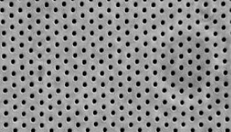
FIG. 1.: A snapshot of the triangular lattice of paramagnetic colloidal particles. A few thousand snapshots such as this, taken at regular time intervals of about one second were used to calculate elastic constants.

In this Letter, we report an experimental determination of the equilibrium elastic properties of two -dimensional (2D) colloidal crystals from “snapshots” of particle positions obtained using video microscopy. The present method is completely non-invasive, accurate and free from any adjustable parameters.

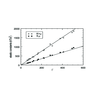
FIG. 2.: The comparison of the measured elastic constants (in units of $kT/a^{2}$, $a$ is the lattice parameter) to the zero-temperature calculation (solid lines) reveals an very good agreement. Note that the shear modulus $\mu$ is multiplied by 5 for reasons of clarity.

The mechanical properties of a macroscopic solid, according to classical elasticity, are well described by a small set of elastic constants. These can be measured by the strain-response of the solid under the application of an appropriate (macroscopic) stress. On a mesoscopic scale, which is still sufficiently coarse-grained to apply elasticity theory but small enough such that the Brownian motion of the particles is observable, thermally induced strain fluctuations can be used to determine elastic constants. We have carried out a detailed study of these strain fluctuations in a two -dimensional (2D) colloidal crystal by recording the microscopic positions of the particles within a square cell (of size $L$) containing a defect -free single crystal (see Fig. 1). Recordings were made at regular time intervals — large compared to typical correlation times of the colloid. Uncorrelated snapshots obtained are analyzed to calculate the average particle positions — the “reference” lattice. The gradients (obtained by finite differences) of the displacement vectors then yield the microscopic strains. These microscopic strains are used to obtain strain fluctuations over a hierarchy of length scales corresponding to smaller sub-cells of size $L_{b}<L$ contained within our cell. The width of the probability distributions of the strains are related to the elastic constants $C_{ijkl}(L_{b})$ obtained as a function of $L_{b}$ which may subsequently be extrapolated, using a systematic finite size scaling analysis[5]. The macroscopic ($L\to\infty$) values of these quantities, thus obtained, are compared to theoretical predictions without any fitting parameters. The central result, the bulk ($K$) and shear ($\mu$) elastic moduli are shown as a function of the interaction strength $\Gamma$ for our colloidal system (see below) in Fig. 2.

Our experimental setup[6, 7] is composed of super - paramagnetic spherical colloids [8] of diameter $d=4.5\,\mu\mbox{m}$ and mass density $1.7\;\mbox{kg/dm}^{3}$. They are confined by gravity to a water/air interface, which is formed by a cylindrical drop suspended by surface tension in a top-sealed ring. The flatness of the water-air interface ($\O=8\;\mbox{mm}$) is controlled within $\pm 1\;\mu\mbox{m}$[6]. For weak magnetic fields $B$ applied perpendicular to the interface the induced magnetic moment $M$ depends linearly on $B$, i.e. $M=\chi B$ with an effective magnetic susceptibility $\chi$[6]. The repulsive magnetic dipole-dipole potential, between particles $i$ and $j$ separated by a distance ${\bf r}_{ij}$, $V(r_{ij})=\Gamma r_{ij}^{-3}$ dominates the interaction and is absolutely calibrated by the interaction strength $\Gamma=(\mu_{0}/4\pi)(\chi B)^{2}(\pi n)^{3/2}/kT$ where $n$ denotes the 2D volume-fraction of the particles, $k$ is the Boltzmann constant, $T$ is the ambient temperature and distances, ${\bf r}_{ij}$, are in units of the mean interparticle spacing.

The experiments were carried out as follows: At high $\Gamma$, in the crystalline phase, the system was equilibrated by the application of small AC magnetic fields in the plane of the particles. Eventually a defect-free crystal containing several thousand particles is obtained. The entire sample consists of approximately $10^{5}$ particles. The coordinates of typically 1000 particles in the (square) field of view were recorded in time. About 500 to 1000 independent coordinate sets, each about a second apart, are necessary to obtain sufficient statistics. The time interval corresponds to diffusion over about 1 micrometer which is about one pixel —- the limit of resolution of our digital camera. The results do not vary significantly over the range of the number of data sets used.

After the determination of the mean position of each particle ${\bf R}^{0}$ (taken over the entire set)[9] the instantaneous displacement $\mathbf{u}(\mathbf{R}^{0})={\bf R}-{\bf R}^{0}$ from the mean position was calculated for each frame and for all particles. The set of coordinates ${\bf R}^{0}$ constitutes, therefore, our reference lattice and the fluctuating displacement variable ${\bf u}({\bf R}^{0})$ is known at every reference lattice point. Once the displacements are known, the elements of the elastic strain tensor $\epsilon_{ij}$ and the local rotation $\theta$ may be defined as gradients of the displacement ${\bf u}$ over the spatial coordinates ${\bf r}$.

$$\varepsilon_{ij}=\frac{1}{2}\left(\frac{\partial u_{i}}{\partial r_{j}}+\frac{\partial u_{j}}{\partial r_{i}}\right)\;\;\;;\;\;\;\theta=\frac{1}{2}\left(\frac{\partial u_{y}}{\partial r_{x}}-\frac{\partial u_{x}}{\partial r_{y}}\right),$$ (1)

When the derivatives are replaced by appropriate finite differences, these quantities may be evaluated at every reference lattice point ${\bf R}^{0}$. In order to evaluate elastic constants, the microscopic strains and rotations need to be coarse-grained or averaged over a sequence of sub-systems (obtained in our case by dividing our square cell into integral numbers of smaller square sub-cells) of size $L_{b}=L/b$, ($b=4,5,..,18$) to obtain size dependent strains and rotations $\epsilon^{b}_{ij}(L_{b})$ (and $\theta_{b}(L_{b})$)

$$\varepsilon^{b}_{ij}(L^{b}),\theta_{b}(L_{b})=\frac{1}{L_{b}^{2}}\int_{L_{b}}\varepsilon_{ij}(\mathbf{r}),\theta({\bf r})\,d\mathbf{r}.$$ (2)

The fluctuations of these quantities for a particular set of sub-systems (all of size $L_{b}$) over the different snapshots yield elastic constants for the size $L_{b}$ from standard thermodynamic relations. Although this procedure has been used[5] for obtaining elastic moduli of the hard and soft disk systems from computer generated configurations, we find that some essential modifications are required before the methods of Ref. [5] can be applied to our system. In a typical computer simulation[5, 10, 11, 12, 13, 14] the system is placed in a hard constraint determined by the ensemble used. For example in a constant (zero) strain ensemble[5] the displacement field ${\bf u}({\bf r})$ strictly vanishes at the boundary so that the strain, integrated over the entire system is strictly zero. Our experimental cell, on the other hand, is a small region embedded within a much larger crystal. The only constraints which are appropriate for this case is that the displacement ${\bf u}$ are continuous throughout the system and ${\bf u}({\bf r})\to 0$ as ${\bf r}\to\infty$. In the limit of linear elasticity for our system where the elastic correlation length is assumed to be much smaller[5] than $L_{b}$, our problem reduces to the determination of the total energy of a single, independent, strain fluctuation in an elastic medium subject to these constraints.

Consider, therefore, a region of size $L_{b}$, with a fixed constant strain (or rotation) $\epsilon^{b}_{ij}(L_{b})$ ($\theta_{b}(L_{b})$) embedded in an (infinite) elastic continuum. This general problem has been studied in detail in several standard texts on classical theory of elasticity[14, 15]. Recall that a 2D hexagonal lattice has isotropic elastic behavior[14] and, therefore, can be completely described by two independent elastic constants, which we choose to be the bulk modulus $K$ and the shear modulus $\mu$. While the former is related to the fluctuations of the volume of the sub-systems the latter may be evaluated from the fluctuations of the angle of rotation of the sub-systems. Let us focus on a small sub-cell within our cell. Consider for the moment that we have a disk of radius $R_{b}$ for simplicity, the final results will be cast in a form independent of the shape of the sub-system. Within this disk, the strains are given by their values which are the averages over the area of the disk. This disk is embedded in an infinite elastic medium with elastic moduli $K$ and $\mu$.

We consider first a homogeneous expansion (or compression) of the disk by $R_{b}\rightarrow R_{b}+\Delta r$. The corresponding radial-displacement $u_{r}$ is given as,

$$u_{r} = \Delta r\cdot r/R_{b},\,\,\,\,r\,\,<R_{b}$$ (3)

$$= \Delta r\cdot R_{b}/r,\,\,\,\,r\,\,>R_{b}$$ (4)

The angular part $u_{\varphi}=0$ by symmetry. The displacements $(u_{r},u_{\varphi})$ are related to the strain tensor by the following equations [15]:

$$\varepsilon_{rr} = \frac{\partial u_{r}}{\partial r}\;\;\;;\;\;\;\varepsilon_{\varphi\varphi}=\frac{u_{r}}{r}+\frac{1}{r}\frac{\partial u_{\varphi}}{\partial\varphi}$$ (5)

$$2\,\,\varepsilon_{r\varphi} = \frac{1}{r}\frac{\partial u_{r}}{\partial\varphi}+\frac{\partial u_{\varphi}}{\partial r}-\frac{u_{\varphi}}{r}$$ (6)

Making use of the (quadratic) free energy density $f$ of the elastic continuum,

$$f = \frac{1}{2}[K(\varepsilon_{rr}+\varepsilon_{\varphi\varphi})^{2}+\mu\{(\varepsilon_{rr}-\varepsilon_{\varphi\varphi})^{2}+4\varepsilon_{r\varphi}^{2}\}]$$ (7)

and integrating $f$ over the entire space, both within and outside the disk (to account for the deformation of the surrounding medium) and using the strains calculated from Eqs.   4 and 6, we get the energy $E=2\pi(K+\mu)\Delta r^{2}$ necessary to expand the disk by $\Delta r$. We may, now, eliminate the shape dependent prefactors by using the volume $V=\pi R_{b}^{2}$ and the volume-change $\Delta V=2\pi R_{b}\Delta r$ of the disk, to obtain finally, the energy $E=(K+\mu)\Delta V^{2}/2V$. Using the equipartition theorem we have therefore,

$$\langle(\Delta V_{b})^{2}\rangle/V_{b}=kT/[K(L_{b})+\mu(L_{b})],$$ (8)

relating the fluctuation of the volume $V_{b}=L_{b}^{2}$ of the sub-cell to the sum of the bulk and shear moduli. The above relation together with $\Delta V_{b}/V_{b}=\varepsilon^{b}_{xx}(L^{b})+\varepsilon^{b}_{yy}(L^{b})$ may now be used to obtain $K(L_{b})+\mu(L_{b})$ for our sub-cells.

A similar treatment leads to a relation between $\mu$ and the local rotation of the system $\theta$ (Eq.1). The rotation of a disk of radius $R_{b}$ by an angle $\theta$ leads to an angular-displacement $u_{\varphi}(r)=\theta\cdot R_{b}^{2}/r$ for $r>R_{b}$ ($u_{\varphi}(r)=0$ for $r<R_{b}$). Applying Eq.  6 and integrating the energy density (Eq.  7) leads to the total energy for the rotation $E=2\pi\mu\theta^{2}R_{b}^{2}$. Equipartition then yields,

$$\mu=\frac{kT}{V_{b}}\frac{1}{\langle(2\theta_{b})^{2}\rangle}.$$ (9)

This equation has precisely the same structure as Eq.  8 and, therefore, similar finite size scaling schemes can be applied. Thus Eq.  9 together with Eq.  8 enable the determination of the elastic constants of the system.

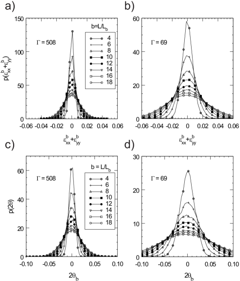
FIG. 3.: (a)and (b)Probability distribution of the box-size averaged strain fluctuations of $\Delta V_{b}/V_{b}=\varepsilon^{b}_{xx}+\varepsilon^{b}_{yy}$ as a function of the (linear) scaling box-size $L_{b}=L/b$ for $\Gamma=508$ (a) and $69$ (b). (c) and (d) Same as in (a) and (b) for the angle $\theta_{b}=\varepsilon^{b}_{xx}-\varepsilon^{b}_{yy}$ for $\Gamma=508$ (c) and $69$ (d). Note the difference in the y-scale between (a) and (b) as well as between (c) and (d)

In Fig.3 the probability distribution of the incremental volume $\Delta V_{b}/V_{b}=\varepsilon^{b}_{xx}+\varepsilon^{b}_{yy}$ and $\theta_{b}$ are shown as a function of the scaled box size $b=L/L_{b}$ for two values of the interaction strength $\Gamma$. The width of the (Gaussian) distributions decreases both with increasing box-size $L_{b}$ and increasing value of $\Gamma$. The mean square fluctuations are obtained by fitting the data to a normal distribution and extracting the standard deviation.

Once the $L_{b}$-dependent elastic moduli are obtained, usual finite size scaling[5] can be used to extrapolate the results to the thermodynamic limit. This is shown in Fig. 4 where we have plotted $L_{b}/L\times 1/[K(L_{b})+\mu(L_{b})]$ as a function of $L_{b}/L$. The slope of the curve, obtained from a straight line fit to the data, gives the value for $1/[K(L=\infty)+\mu(L=\infty)]$. A similar finite size scaling is used to obtain $\mu(L=\infty)$ separately. These results are shown in Fig.2 both for $K+\mu$ – as obtained from Eq.8 – and for $\mu$ from Eq.9 as a function of the interaction strength $\Gamma$. Note the accuracy of the determination of the elastic moduli for our system which is facilitated by the fact that the interaction potential $\Gamma$ of our system is precisely calibrated. The straight lines through our data in Fig.2 are the results from a $T=0$ calculation of the elastic constants of a 2D triangular solid composed of particles interacting with an inverse cubic potential[16]. For all inverse power potentials the $T=0$ limit is exact to lowest order[17]. Considering the deformation of a perfect static triangular solid of particles interacting with a $r^{-3}$ potential one obtains the relation $\mu=K/10$ and the numerical result $K=3.461\cdot\Gamma$, where the numerical coefficient is evaluated by performing a rapidly convergent lattice sum. The agreement is excellent (considering the fact that no fitting parameter is available) over a wide range of interaction strengths $\Gamma$ down to values of 70 – the melting transition occurs at $\Gamma=60$ [7].

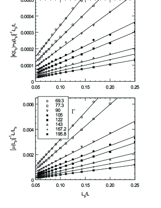
FIG. 4.: Finite size scaling behavior of $[K(L_{b})+\mu(L_{b})]^{-1}\cdot L_{b}/L$ (top) and $\mu(L_{b})^{-1}$ as a function of $L_{b}/L$ dependent on the interaction strength $\Gamma$. A straight line fit to the curves gives the infinite system values of the (inverse) moduli.

Finally, a few words on the possible uncertainties involved in our determination of the elastic moduli seem to be in order. Firstly, we have neglected all fluctuations of the magnetic moment, both in amplitude and angle. Since a super-paramagnetic colloid particle is of macroscopic dimensions compared to typical magnetic length scales this assumption seems to be justified. Secondly, we have assumed that the particles fluctuate on a flat, two -dimensional air-water interface. An estimate[6] of the out-of-plane fluctuations is given by the ratio of the gravitational length $l_{g}=kT/mg$ (where $m$ is the mass of the particles and $g$ is the acceleration due to gravity) and the interparticle spacing; this is typically $1$ in $10^{3}$. Lastly, a possible limitation of this scheme, at least in its present form, is the requirement that the displacement field u(r) be analytic in order to obtain strains by taking derivatives. Therefore one needs to restrict analysis to dislocation free regions of the sample — which is possible only if the system is sufficiently far away from a melting transition[7]. Suggestions[5, 12] to circumvent this problem are, however, computationally difficult to implement. The study of elastic properties of paramagnetic colloids in the presence of obstacles and inclusions, as well as dynamical elastic response is an interesting direction for further research. This is particularly suited for our technique since it provides a local (and therefore precise) probe[4] for elastic properties.
Acknowledgements:The authors thank M. Rao for a critical reading of the manuscript. One of us (S.S.) thanks the Alexander von Humboldt Foundation. Support by the Deutsche Forschungsgemeinschaft in the frame of the Sonderforschungsbereich 513 is kindly acknowledged.

REFERENCES

- [1] P. N. Pusey, in Liquids, Freezing and the Glass Transition, edited by J. P. Hansen, D. Levesque and J. Zinn-Justin (North-Holland, Amsterdam, 1991).
- [2] Schöpe H.J. et al., J. Chem. Phys. 109 22, 10068 (1998)
- [3] Palberg T. et al., J. Phys. III 4, 457 (1994)
- [4] A. Wille, F. Valmont, K. Zahn and G. Maret, Euro. Phys. Lett. 57, 210 (2002).
- [5] S. Sengupta, P. Nielaba and K. Binder, Phys. Rev. E 61, 1072 (2000).
- [6] K. Zahn, J.M. Méndez-Alcaraz, G. Maret, Phys. Rev. Lett. 79, 175 (1997).
- [7] K. Zahn, R. Lenke and G. Maret, Phys. Rev. Lett. 82, 2721 (1999)
- [8] Dynabeads M-450, uncoated; Deutsche Dynal GmbH Postfach 111965 D-20419 Hamburg.
- [9] This is not in conflict with the divergence of the mean square displacement in 2D crystals, which is only valid in the thermodynamic limit. For finite systems, however, the equilibrium position of the particles are well defined also in 2D systems.
- [10] M.Parrinello and A. Rahman, J. Chem. Phys. 76(5), 2662 (1982).
- [11] K.W. Wojciechowski and A.C. Branka, Phys. Lett. A 134, 314 (1988).
- [12] S. Sengupta, P. Nielaba and K. Binder, Phys. Rev. E 61, 6294, (2000).
- [13] D.H. Wallace, in Solid State Physics, edited by H. Ehrenreich, F. Seitz and D. Turnbull (Academic Press, New York, 1958).
- [14] L.D. Landau and E.M. Lifshitz, Theory of Elasticity, 3rd ed. (Pergamon, Oxford, 1986).
- [15] H.G. Hahn, Elastizitätstheorie (B.G. Teubner, Stuttgart, 1985).
- [16] A. Wille, PhD thesis, University of Constanz, Germany, (2001).
- [17] B. J. Alder, W. G. Hoover and D. A. Young, J. Chem. Phys. 49, 3688 (1968).