Time evolution of damage under variable ranges of load transfer

Abstract

We study the time evolution of damage in a fiber bundle model in which the range of interaction of fibers varies through an adjustable stress transfer function recently introduced. We find that the lifetime of the material exhibits a crossover from mean field to short range behavior as in the static case. Numerical calculations showed that the value at which the transition takes place depends on the system’s disorder. Finally, we have performed a microscopic analysis of the failure process. Our results confirm that the growth dynamics of the largest crack is radically different in the two limiting regimes of load transfer during the first stages of breaking.

I Introduction

The phenomenon of fracture in heterogeneous materials is a complex physical problem which has been of great interest to scientists for quite a long time r1 ; r2 ; r3 . A disordered system is understood to be one with random time or/and space dependent breaking properties r1 . The random nature of this dependence arises because modeling the fracture of heterogeneous materials entails dealing with systems made up of many constituents, each one having mechanical properties that can be considered as being independent of the properties of the other constituents, but with many body interactions among the different parts of the system r1 ; r2 ; r3 . In heterogeneous materials the evolution of the rupture process is radically different from the single crack growth mechanism that occurs in homogeneous materials. Though there is neither a complete numerical solution nor analytic solution to the fracture problem, we have a better understanding of it due to some recent algorithms that have been developed to simulate the fracture process r4 ; r5 ; r6 ; r7 ; r8 .

Fiber Bundle Models (FBM) form a fundamental class of approaches to the fracture problem. They arose in close connection with Daniels’ and Coleman’s seminal works on the strength of bundles of textile fibers r9 ; r10 , and have harbored an intense research activity in recent years r1 ; r2 ; r3 ; r4 ; r11 ; r12 ; r13 ; r14 ; r15 ; r16 ; r17 ; r18 ; r19 ; r19b ; r19c . Fiber Bundle Models are important, despite their very simple nature, because they exhibit most of the essential aspects of material breakdown. In addition, the deep understanding of fracture processes they provide has served as a starting point for more complex models r13 ; r14 ; r15 ; r19a ; r20 ; r21 . In FBMs the material is made up of a set of parallel fibers, each having a statistically distributed threshold strength or life-time. Besides the classical static FBM one can also introduce a dynamic version r18 . In the static FBM, the failure process is simulated according to a quasi static loading of the material in which the output of the simulation is the ultimate strength of the material, i.e, the maximum load above which it breaks down. In the dynamic FBM, a constant load is maintained on the system and the fibers break by fatigue after some time.

After a fiber breaking, the load acting on it is redistributed among the intact fibers according to the stress redistribution rule associated with the particular load-transfer model. There are two standard load transfer models comprising the FBM and they correspond to the extreme limits of stress redistribution. The global load sharing (GLS) redistributes the load of a failed fiber equally among the active fibers remaining in the system. It is known as the global fiber bundle model (GFBM), and assumes long-range interaction among the fibers which makes it a mean-field approximation that can be solved analytically r11 ; r12 . On the other hand, the local load sharing (LLS) redistributes the load of a failed fiber among the intact fibers that are nearest neighbors to the failed ones, and is thus known as the local fiber bundle model (LFBM). This assumes short-range interaction among the fibers and it has not, in general, been solved analytically. However, in actual heterogeneous materials the stress redistribution is expected to fall in between the two regimes of load transfer. Very recently, some of us have proposed a load transfer scheme with variable range of interaction among the fibers, which interpolates between the two extreme cases. Since most of the physics of the fracture problem is hidden in the stress redistribution, considering within the same model the possibility of varying the range of interaction is a relatively greater improvement toward a better understanding of the fracture problem.

Motivated by the results obtained for the static setting, we have studied a stochastic dynamic fiber bundle model, in which fibers break by fatigue over a period of time, such that the range of interaction among fibers is variable through an adjustable stress transfer function. We have observed a crossover from mean-field to short-range behavior for the macroscopic quantities describing the fracture dynamics as in the static case. In addition, a more detailed inspection of the failure process revealed that the microscopic behavior of the system is also different as the range of interaction varies. Finally, we have also studied the effect of heterogeneity on the failure process from macroscopic as well as microscopic perspectives. The rest of the paper continues with the description of the stochastic model in the next section. Section III is devoted to study the lifetime of the bundle and the rate at which fibers break when the range of interaction changes. The damage spreading for several load transfer modalities is addressed in section IV while the last section is devoted to conclusions rounding off the paper.

II The stochastic model.

We assign each fiber to the sites of a square lattice, with periodic boundary conditions. Assuming elastic interaction among the fibers, we may state that the stress redistribution obeys a power law r21 ,

$$\sigma_{inc}{\sim}\frac{1}{r_{ij}^{\gamma}},$$ (1)

where $\sigma_{inc}$ is the load increment on an intact fiber $i$ at a distance $r_{ij}$ from the failed fiber $j$, and $\gamma$ is a variable parameter that controls the effective range of interaction among the fibers. $\gamma$=0 corresponds to GLS since the additional load on each intact fiber as a result of a fiber breaking is the same irrespective of its distance from the broken fiber. On the other hand, $\gamma=\infty$ corresponds to LLS since in this limit only the nearest neighbors get equal portions of the load of a failed fiber, and $\sigma_{inc}$=0 for $r>1$. Assuming that there is no dissipation of the load of a failed fiber, Eq. (1) leads us to the normalized stress transfer function,

$$S(\gamma,r_{ij})=\frac{1}{r_{ij}^{\gamma}}\frac{1}{\sum_{i\in{A}}r_{ij}^{-\gamma}}$$ (2)

$r_{ij}$ being the distance between an active fiber $i$, with coordinates $(x_{i},y_{i})$, and a failed fiber $j$, with coordinates $(x_{j},y_{j})$, and $A$ denotes the set of intact fibers.

One can consider two equivalent approaches to the dynamic FBM r22 ; r23 ; r24 . The time elapsed until the final collapse of the system is the lifetime or time to failure of the bundle. In the first approach r22 the lifetime of each element is an independent identically distributed random variable, i.e, each fiber has a different random lifetime, taken from the same statistical distribution (the Weibull distribution is a good empirical distribution in materials science) and each one breaks if the time elapsed exceeds its individual lifetime. This is a quenched model of fracture where the disorder is introduced once for all at the beginning of the process and thus the growth mechanism is deterministic. In this version, the effect of the increase in stress for a particular fiber $i$ due to the redistribution of load from failed fibers is the reduction of its initially assigned lifetime $t_{i}$ to a new lifetime $\tau_{i}$ given by

$$t_{i}=\int_{0}^{\tau_{i}}\left(\frac{\sigma_{i}(t)}{\sigma_{0}}\right)^{\rho}dt,$$ (3)

where $\sigma_{0}$ is the initial stress on fiber $i$ at $t=0$ and $\rho$ is the Weibull index, $2\leq\rho\leq 50$. $\rho$ gives the degree of heterogeneity of the system; as $\rho$ increases the system becomes more homogeneous. In this model the next element to break is exactly the one with the lowest lifetime at time $t$.

In the probabilistic approach r23 ; r24 , it is considered that in a time step all the intact elements have the same mean time to failure. The element that breaks in the time interval between two successive failures is selected by chance and thus the fiber whose probability of breaking (a function of the load it bears) is the largest is more likely to fail. The probabilistic approach is an example of the so called annealed disorder since the algorithm is stochastic and thus randomness is uncorrelated in time. Thus, we start at time $t=0$ with $N$ fibers loaded with an initial common stress of $\sigma_{i}(t)=\sigma_{i}(0)=1$. The mean time interval $\delta$ for an individual element to break by fatigue is,

$$\delta=\frac{1}{\sum_{i\in{A}}\sigma_{i}^{\rho}(t)},$$ (4)

where $A$ is the set of intact fibers and $t$ is the time elapsed up to $k-1$ breakings, i.e., $t=\sum_{p=1}^{k-1}\delta_{p}$. In the first time interval where $\sigma_{i}=1$ $\forall i$, with all the $N$ elements active, $\delta_{1}=\frac{1}{N\sigma_{i}^{\rho}}$ so that the first fiber breaking is completely random. This changes with time due to stress transfers and fiber failures. The probability of a particular fiber breaking $j$ in one sweep of the lattice in the time interval $\delta_{k}$, is given by

$$P_{j}(t)=\sigma_{j}^{\rho}(t)\delta_{k}.$$ (5)

When a fiber breaks, its load is transfered and as a consequence, the probability of failure of the receptors is increased. In this sense there are no weak or strong fibers, all the fibers are equivalent but carrying different loads (except for mean field approaches) and thus with different breaking probabilities. It is worth stressing that both approaches are equivalent. This can be intuitively understood by noting that in both models the load history plays a key role. For the quenched setting the fiber that breaks is that with the lowest lifetime which in its turn depends on the load history. Since the individual times to failure are reduced each time a fiber receives load from a failed element, the more stressed a fiber is, the more likely its lifetime is the lowest. On the other hand, for the annealed version the magnitude that is modified by the load redistribution is the probability of breaking and the load history affects the failure process just as in the deterministic version: the more stressed a fiber is, the more likely it breaks. Additionally, we note that this algorithm is the same as the one used in polymer failure pol and in describing dielectric breakdown db with the main distinction that here the broken fibers need not to be connected to the single growing cluster as in dielectric breakdown.

Now, the load born by the fiber that has just failed is redistributed according to Eq. (1) such that in a time interval $\Delta t=t_{k}-t_{k-1}=\sum_{p=1}^{k}\delta_{p}-\sum_{p=1}^{k-1}\delta_{p}=\delta_{k}$, the load increase on the active fiber $i$ reads as

$$\sigma_{i}(t_{k})=\sigma_{j}(t_{k-1})S(\gamma,r_{ij})+\sigma_{i}(t_{k-1}),$$ (6)

where $\sigma_{j}$ is the load of the element that has failed in the time interval ${\Delta}t$ after $k$ fiber failures. After the redistribution of load the rupture process continues by applying again Eq. (5) that will point to the next fiber to break. The lifetime of the material is then given by the sum of all the $N$ $\delta$s, $T_{f}=\sum_{i=1}^{N}\delta_{i}$.

The complete analytic solution to the dynamic FBM as defined above in the GLS ($\gamma=0$) case is feasible. The lifetime of the material can be computed as

$$T_{f}=\int_{1}^{N}\frac{(N+1-x)^{\rho-1}}{N^{\rho}}dx=\frac{1}{\rho}\left[1-\frac{1}{N^{\rho}}\right]$$ (7)

that includes also the dependence of the lifetime on the system size $N$ giving the mean field result $1/\rho$ in the thermodynamic limit.

We should note that there is no avalanche here, unlike to the static case r21 , since there is no external driving on the system. Once the fibers start breaking by fatigue, they continue breaking with time until the final collapse of the system, but within a time interval $\delta_{k}$, only one fiber may break in a single sweep of the lattice.

We note that both Eqs. (3) and (5) assume a power-law breaking rule $\kappa_{p}(\sigma)=\nu_{0}(\sigma/\sigma_{0})^{\rho}$. This stems from the former assumption that the lifetimes satisfy the Weibull distribution. An alternative breaking rule could be and exponential hazard rate of the form $\kappa_{e}(\sigma)=\phi\exp(\eta(\sigma/\sigma_{0}))$ mainly used for thermally activated processes. On the other hand, $\kappa_{p}$ has the same functional form as the Charles power law that describes the subcritical crack growth induced by stress corrosion in geological materials at constant temperature: $v=AK_{I}^{n}$, where $v$ is the crack velocity and $K_{I}$ is the stress intensity factor for mode $I$ fracture. Sometimes, $n$ is known as the stress corrosion index. Moreover, we emphasize that Eq. (4) is not a real measure of time so that a quantitative comparison between the results here shown and those from experiments is not feasible. Additionally, Eq. (4) is a simple form one can consider for the probability of breaking. In principle, one could also include more realistic rules. Nevertheless, as we shall see, this simple model is very rich and might help understand physical effects present in real materials.

III Lifetime of the bundle

We simulate the failure process by large scale numerical simulations. We first explore the behavior of the lifetime as a function of the stress transfer range for a fixed level of heterogeneity ($\rho=2$). Then we vary the Weibull index such that we get a more homogeneous system with smaller times to failure.

Figure 1: Lifetime $T_{f}$ versus effective range of interaction $\gamma$. The crossover from mean-field to short-range behavior is obtained at the same transition point as in the static case ($\rho=2$).

The results obtained for the lifetime are depicted in Fig. 1 for different values of the range of interaction among the fibers and several system sizes up to $N=6400$ fibers. A crossover from mean field behavior to a regime dominated by the short range interactions among the fibers is clearly appreciated. Furthermore, the critical value of the parameter $\gamma_{c}$ defines a region where the results for global load sharing models hold beyond $\gamma=0$, the true mean-field regime for which the load of a failed element is shared equally among the surviving elements. For $\gamma\leq\gamma_{c}$ the material behaves macroscopically as for $\gamma=0$, that is, the lifetime is independent on the system size and does not depend on the actual value of the exponent $\gamma$. It is not a simple numerical task to determine accurately the exact value of the transition point due to the stochastic nature of the model and the fluctuations of the lifetime of the system. In fact, the time to failure of the bundle follows a Gaussian distribution in what concerns its frequency distribution. The width of the distribution depends on the level of heterogeneity (controlled by the Weibull index) that in turn also influences the lifetimes that become shorter as we move to high levels of homogeneity. Within this numerical uncertainty we have found that $\gamma_{c}\sim 2$. Interestingly, the same value was found to characterize the transition of the bundle’s ultimate strength from long to short range behavior in the static case of the model r21 .

Figure 2: Comparison of the time to failure obtained for different heterogeneity levels $\rho$ as the range of interaction varies. The inset corresponds to $\rho=5$ while the main figure has been drawn considering $\rho=10$. Clearly, the crossover behavior is still present although the value of the transition point depends on $\rho$. As the system gets more homogeneous, $\gamma_{c}$ shifts leftwards.

The influence of the disorder on the crossover behavior can be studied by changing the value of $\rho$. Fig. 2 shows the time to failure of the material as a function of the effective range of interaction for several system sizes. We observe that the transition is still present but the range where the mean field regime applies is reduced. In particular, as the system gets more homogeneous $\gamma_{c}$ shifts leftwards to smaller values. Additionally, the true local load sharing regime appears to be also slightly shifted to the left. When the range of interaction $\gamma$ falls below a second transition point $\gamma_{c2}$, the lifetime of the bundle becomes again independent on the effective interaction among the fibers but it is still size dependent. This later behavior can be easily understood by noting that for local load sharing schemes the time to failure of the system in the thermodynamic limit is zero. We have checked that in our model this is actually verified, although the drop of the lifetime as the system size is increased is slow. On the other hand, wherever the GLS regime arises, the time to failure of the system is not size dependent for large $N$ (see Eq. (7).)

Another way to characterize the evolution of the fracture process is to inspect the rate at which fibers fail. We expect two different asymptotic regimes. For long range interaction, i.e., below $\gamma_{c}$ the system should behave in a mean field manner. This means that damage is gradually accumulated in the material up to a point in which the load is too high as to be carried by the remaining fibers. Only at this stage of the damage process the rate of fiber failures will speed up owing to the small values of the very last $\delta$s. On the contrary, in the region where short range interaction prevails, the system does not accumulate damage uniformly. In this case there appear regions within the material in which stress enhancement takes place making the fibers along the crack tips to support much more load than other active fibers placed far from the clusters of broken fibers.

Figure 3: Normalized number of broken fibers as a function of time (also normalized to the lifetime of the bundle). Two groups of curves can be clearly distinguished corresponding to the long range and short range regimes. The results have been obtained for a system of $N=2500$ fibers and $\rho=2$.

Accordingly, the $\delta$s would be modified and there would be more breakings for the same time interval. In other words, the breakdown of the material occurs suddenly for the very localized regime where about $50\%$ of the fibers breaks in a time interval of the order of $0.1T_{f}$. In Fig. 3 we have represented the evolution with time of the number of broken fibers $N_{f}$ for different values of $\gamma$. Two distinct groups of curves corresponding to the extreme cases can be clearly seen. For intermediate values of the effective range of interaction, the behavior is more like the case of long range interaction and may correspond to other load sharing schemes such as the hierarchical fiber bundle model r18 ; r25 .

Consider that the breaking rate of the bundle is defined as

$$r(t)=\frac{dN_{f}(t)}{dt},$$ (8)

with $N_{f}(0)=0$ and $N_{f}(T_{f})=N$. Upon approaching the complete failure, the breaking rate scales with the lifetime of the material as r26

$$r(t)\sim(T_{f}-t)^{-\zeta},$$ (9)

where the exponent $\zeta$ depends on both the range of interaction and the Weibull index. However, we can again identify two limiting groups of curves for the same value of $\rho$. Figure 4 shows the rate of fiber breaking for several load transfer ranges and a Weibull index $\rho=2$. These results confirm the behavior observed for the evolution of the number of broken fibers, namely that there is a sharp increase in the failure rate when approaching the lifetime for the case where short-range interaction dominates the damage spreading. The fit to the curves gives $\zeta\approx 1/2$ for $\gamma\leq\gamma_{c}$ and $\zeta\approx 2/3$ when $\gamma$ is in the range where the effective interaction among the fibers can be assumed to be very localized. Note that the curves for intermediate values of $\gamma$ and for the GLS regime have been shifted for the sake of clarity. The numerical results are not very smooth because of fluctuations but the general trend of $r(t)$ confirms the validity of relation (9). As to the dependence of the above results on the heterogeneity level we have observed that the less heterogeneous the material is, the sharper the failure acceleration is in all cases.

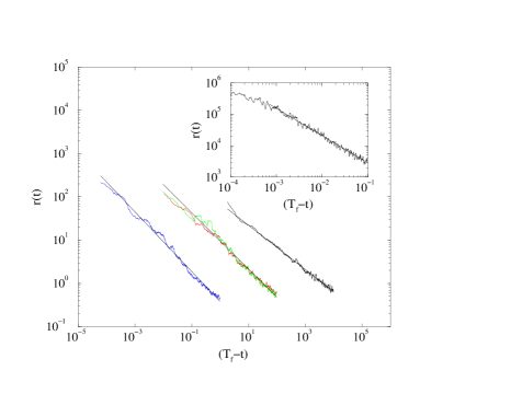
Figure 4: Scaling of the breaking rate $r(t)$ (as defined in the text) when approaching the time of material’s breakdown. The values of $\gamma$ are, from right to left, $0$, $4$, $5$, and $20$. With the exception of $\gamma=20$, the curves have been shifted to the right for the sake of clarity. The least square fit to the data gives for the exponent the values $\zeta(\gamma=0)=0.5\pm 0.02$, $\zeta(\gamma=4)=\zeta(\gamma=5)=0.58\pm 0.02$ and $\zeta(\gamma=20)=0.66\pm 0.02$. The values of $N$ and $\rho$ are as of Fig 3. The inset shows the same quantity for $\gamma=0$ and $\rho=10$. The scaling exponent is in this case $\zeta=0.86\pm 0.02$.

The inset in Fig. 4 shows the breaking rate for the case of long range interaction and $\rho=10$. The higher value of $\zeta\approx 0.86$ indicates that much of the fibers break in a very small time interval close to the lifetime of the material. As the range of interaction gets more localized, the exponent $\zeta$ approaches unity.

IV Crack growth

A further characterization of what is going on in the fracture process can be carried out by focusing on the properties of the clusters of broken fibers. Specifically, we have monitored the growth of the cracks inside the bundle. Cracks are defined as connected clusters or regions of broken fibers. Here, we consider a coordination number $q=8$, that is, each fiber has 8 neighbors. Similar results are obtained if we take into account only nearest neighbors ($q=4$). At the very initial stages, regardless of the range of interaction among the fibers, the failure of fibers can be assumed to be random, that is, the initial cracks are randomly nucleated inside the material. This situation changes with time for different load transfer schemes. By studying the growth of the largest crack area $C_{m}$ at each time step, one could distinguish the different mechanisms leading to the rupture of the material as the range of interaction varies. It is worth noting that this is just a way that allows to discern between different ranges of interaction and levels of heterogeneity. For instance, one can consider instead the linear size of the largest crack and study the fractal dimension of the crack distribution for different $\rho$.

Figure 5 shows a microscopic aspect of the material breakdown with time for the two limiting cases of load redistribution and a system consisting of $N=900$ fibers ($\rho=2$). Initially, it can be seen that cracks are randomly nucleated in the material. At later times the individual microcracks coalesce thereby causing a jump in the largest crack area. For long range interaction, the nucleation of cracks continues to be random because all the fibers carry the same load and thus they break by chance. Therefore the largest broken cluster does not grow linearly with the number of broken fibers. In this case, there are isolated cracks inside the material that grow essentially by coalescence when they meet each other. This is the reason why sudden jumps in the area of the largest crack are observed in the intermediate stages of the damage spreading. At the end of the process, the material has accumulated many of these cracks giving rise to the linear crack growth shown in the inset.

Figure 5: Growth of the largest crack area $C_{m}$ with increasing number of failed fibers $N_{f}$ for the two extreme load sharing rules here illustrated for $\gamma=0$ (long range interaction) and $\gamma=20$ (short range interaction). The bundle consists of $N=900$ fibers and $\rho=2$. The straight line is a fit to the form $C_{m}=aN_{f}$ with $a=0.90\pm 0.04$. The inset shows the evolution of $C_{m}$ up to the macroscopic breakdown of the system for the same set of parameters.

For localized range of interaction, the mechanism of damage spreading is radically different. Again, at small times, the cracks are randomly nucleated inside the material. However, as time goes on and more fibers get broken, the load is redistributed to the fibers located along the crack tips provoking the accumulation of stress in these fibers and the appearance of regions where fibers bear a huge amount of load. It is thus expected that the newly broken fibers add to already existing cracks and that a dominant crack appears. From this perspective, the largest crack area should scale linearly with the number of broken fibers, i.e., $C_{m}\approx N_{f}$. This is indeed the case for $\gamma=20$ as represented in Fig. 5. The straight line is a linear fit to a time window in which more than 150 fibers have been broken. The value $0.90$ of the slope confirms the above picture. Note that in this case the number of coalescence events is smaller than for the GLS regime and that after one of such events the linear growth of the largest crack is recovered. We also note that, up to the intermediate stages of the rupture process, the largest crack for a given number of failed fibers is much higher in the localized case than the global case indicating the formation of a (few) dominant crack(s) in the later case. Additionally, at the end of the process there are no differences between the two extreme load transfer schemes since more than a half of the material is already broken and is very unlikely to find a region where isolated cracks can be formed and grow. Thus, at the final stage each additional breaking event occurs at the crack tips of existing single dominant cracks. Nevertheless, as stated in the previous section the rate of fiber failures is quite different in both asymptotic regimes. We shall note here that the same behavior as for the mean field regime is observed for any value of $\gamma$ provided it is below the transition point $\gamma_{c}=2$.

Figure 6: Growth of the largest crack area $C_{m}$ with increasing number of failed fibers $N_{f}$ for the local load sharing regime here illustrated for $\gamma=10$ and several heterogeneity levels. The bundle consists of $N=900$ fibers. The inset shows the evolution of $C_{m}$ for the long range interaction regime ($\gamma=0$) and the same levels of heterogeneity.

Figure 6 further substantiates our previous arguments by showing how the largest crack area varies as a function of the number of broken fibers for several levels of heterogeneity. While for $\gamma=0$ the picture is always the same (inset), for $\gamma=10$, that is, in the localized regime, the time taken for cracks to become dominant decreases with increasing $\rho$. Furthermore, when the system is very homogeneous ($\rho=10$) and local interactions prevail, a dominant crack which grows until the material collapses is formed almost instantaneously confirming that the mechanism of rupture and crack growth for homogeneous materials is radically different from that of heterogeneous systems. Nevertheless, for the global load case, the change in system’s homogeneity does not alter the way dominant cracks appear and grow (see the inset, where no changes, apart form statistical fluctuations, can be observed). The reason why this happens is given by the way the system gets broken. Equation (5) tell us that the more stressed a fiber is, the more likely it breaks. This always holds except for the global load sharing case, where the fibers share the same amount of load and thus all of them have the same probability to break. As the system is more homogeneous (larger $\rho$), for local load sharing schemes, the probability of breaking for the same load is higher so that the appearance of a dominant crack is enhanced. Therefore, for long range interaction there is no correlated crack growth while for short range regimes this is precisely the dominant mechanism since the first stages of the damage spreading.

V Conclusions

We have extended the fiber bundle model with variable range of interaction between fibers to the dynamic setting. As for the static version, two very different regimes are identified as the exponent of the stress transfer function varies. The lifetime of the material for $\gamma<\gamma_{c}$ does not depend on both the system size and $\gamma$ qualifying for a mean field behavior. On the contrary, for the short range regime, the time to failure of the system systematically decreases when increasing the size of the bundle. The analysis performed also showed that the exact value of the crossover point depends on the level of heterogeneity of the system. Besides, we investigated how the material approaches its point of total breakdown at both sides of the crossover point. The crossover from one regime to the other also influences the behavior of the rate at which fibers break, explicitly manifested in a power law divergence as $T_{f}$ is approached, but with an exponent that depends on the range of interaction. This result is relevant from a practical point of view since for the localized regime the acceleration of the failure process takes place at the very final stages of the rupture process. Although fibers break by fatigue, one by one, they do break in very different time intervals according to the range of interaction. In this sense, a global load sharing regime is safer, since we get more warnings before the material breakdown. On the other hand, the precursory activity when the range of interaction gets localized is almost absent leading to a sudden breakdown of the bundle in a very short time interval.

The numerical exploration of the damage spreading mechanisms under different load transfer regimes further supported the results obtained for the lifetime of the system. Regardless of the range of interaction, the breaking of fibers is a completely random process at the initial stages of the failure process. After some time, the mechanism of failure propagation radically changes when the exponent $\gamma$ varies. In the limiting case of global load sharing there is no correlated crack growth in the system, whereas for the short range regime the damage spreading is driven by a dominant crack, and thus, the crack growth is strongly correlated with high stress concentration at the fibers located along the perimeter of the dominant cluster of broken fibers.

Figure 7: Snapshots of the clusters when nearly $40\%$ of the system is broken. The bundle consists of $900$ fibers and the parameters of the model are shown above the figure. Note that varying the heterogeneity level for $\gamma=0$ does not alter the way in which nucleation and crack growth take place. For localized regimes, as the system gets more homogeneous, the dominant crack appears at early stages and drives the whole breakdown of the material.

These differences are clearly appreciated in Fig. 7, where we represent snapshots of the lattice when nearly $40\%$ of the system is broken for several values of $\gamma$ and $\rho$. For the long range interaction limit the material’s level of heterogeneity does not influence the random nucleation and growth of cracks and there are no clearly distinguishable dominant cracks. This continues to be so until coalescence drives the further breaking of the material. On the contrary, for localized regimes (left column in Fig. 7), when the system gets more homogeneous the dominant crack appears at early stages and damage spreading is strongly correlated resembling a single crack growth mechanism typical of homogeneous materials. When the bundle is heterogeneous, crack growth is still correlated, but in this case we can identify more than one large and dominant crack. Finally, our results suggest that actually there are only two limiting cases relevant to experiments. The one in which mean field assumptions apply could be of great importance since this will allow the extension of known analytic results to ranges of interaction beyond $\gamma=0$.

VI Acknowledgments

One of the authors (Y. M. ) would like to thank A. F. Pacheco and J. B. Gómez for valuable comments on this work. O. E. Y. thanks the ICTP and UNESCO for their financial support and hospitality. Y. M. acknowledges financial support from the Ministerio de Educación Cultura y Deportes (Spain) and of the Spanish DGICYT Project BFM2002-01798. F. K. acknowledges financial support of the Bólyai János Fellowship of the Hungarian Academy of Sciences and of the Research Contracts FKFP 0118/2001 and T037212. This work was partially supported by the project SFB381, and by the NATO grant PST.CLG.977311.

References

- (1) Statistical Models for the Fracture of Disordered Media, edited by H. J. Herrmann and S. Roux (North Holland, Amsterdam, 1990),and references therein.
- (2) Critical Phenomena in Natural Sciences, edited by D.Sornette (Springer-Verlag, Berlin, 2000), and references therein.
- (3) Statistical Physics of Fracture and Breakdown in Disordered Systems, edited by B. K. Chakrabarti and L. G. Banguigui (Clarendon Press Oxford, 1997), and references therein.
- (4) D. Stauffer and A. Aharony, Introduction to Percolation Theory, 2nd ed. (Taylor and Francis, London, 1994)
- (5) M. Sahimi, Applications of Percolation Theory (Taylor and Francis, London, 1994)
- (6) L. deArcangelis, S. Redner, and H. J. Herrmann, J.Phys. (France) Lett.46, L585 (1985).
- (7) S. Feng and P. N. Sen, Phys. Rev. Lett.52, 216 (1984); Y. Cantor and I. Webman, ibid. 52, 1891 (1984).
- (8) S.Roux, and E. Guyon, J. Phys. (France) Lett. 46, L999 (1985).
- (9) H. E. Daniels, Proc. R. Soc. London, A 183, 405 (1945).
- (10) B. D. Coleman, J. Appl. Phys. 28, 1058 (1957); 28, 1065 (1957).
- (11) D. Sornette, J. Phys. I (France) 2, 2089 (1992).
- (12) P. C. Hemmer, and A. Hansen, J. Appl. Mech. 59, 909 (1992).
- (13) C. Moukarzel, and P. M. Duxbury, J. Appl. Phys. 76, 1 (1994).
- (14) D. G. Harlow, and S. L. Phoenix, J. Compos. Mater. 12, 195 (1978).
- (15) R. L. Smith, and S. L. Phoenix, J. Appl. Mech. 48, 75 (1981).
- (16) S. Zapperi, P. Ray, H. E. Stanley, and A. Vespignani, Phys. Rev. Lett. 78, 1408 (1997).
- (17) Y. Moreno, J. B. Gómez,and A. F. Pacheco, Phys. Rev. Lett. 85, 2865 (2000).
- (18) M. Vázquez-Prada, J. B. Gómez, Y. Moreno, and A. F. Pacheco, Phys. Rev. E 60, 2581 (1999).
- (19) W. A. Curtin, Phys. Rev. Lett. 80, 1445 (1998).
- (20) S. Pradhan, P. Bhattacharyya, and B. K. Chakrabarti, Phys. Rev. E 66, 016116 (2002).
- (21) S. R. Pride, and R. Toussaint, Physica A 312, 159 (2002).
- (22) F. Kun, S. Zapperi, and H. J. Herrmann, Eur. Phys. J. B 17, 269( 2000).
- (23) L. Moral, Y. Moreno, J. B. Gómez,and A. F. Pacheco, Phys. Rev. E 63, 066106 (2001).
- (24) R. C. Hidalgo, Y. Moreno, F. Kun, and H. J. Herrmann, Phys. Rev. E 65, 046148 (2002).
- (25) W. I. Newman, D. L. Turcotte, and A. M. Gabrielov, Phys. Rev. E 52, 4827 (1995).
- (26) J. B. Gómez, Y. Moreno, and A. F. Pacheco, Phys. Rev. E 58, 1528 (1998).
- (27) Y. Moreno, A. M. Correig, J. B. Gómez,and A. F. Pacheco, J. Geophys. Res. B 106, 6609 (2001).
- (28) Y. Termonia, P. Meakin, and P. Smith, Macromolecules 18, 2246 (1985).
- (29) L. Niemeyer, L. Pietronero, and H. J. Weisman, Phys. Rev. Lett. 52, 1033 (1984); L. A. Turkevich and H. Scher, Phys. Rev. Lett. 55, 1026 (1985).
- (30) W. I. Newman, A. M. Gabrielov, Int. J. Fract. 50, 1 (1991).
- (31) S. D. Zhang, Phys. Rev. E 59, 1589 (1999).