Finite-Size Effects in a Supercooled Liquid.

Abstract

We study the influence of the system size on various static and dynamic properties of a supercooled binary Lennard-Jones liquid via computer simulations. In this way, we demonstrate that the treatment of systems as small as $N=65$ particles yields relevant results for the understanding of bulk properties. Especially, we find that a system of $N=130$ particles behaves basically as two non-interacting systems of half the size.

I Introduction.

The theoretical understanding of the glass transition is still far from being complete. During the last years, though, considerable progress has been made both from the analytical and the numerical side (see, e.g., reference Debenedetti and Stillinger (2001)). In this paper, we will dwell on some questions that arise within the framework of the energy landscape approach Goldstein (1969); Stillinger (1995). The beauty of this viewpoint lies in the fact that the complicated nature of many-particle effects in structurally disordered matter can be formulated in a pictorial way by considering the topology of the high-dimensional landscape of the total potential energy $V(x)$ (PEL). (Here, $x=(\mathbf{x}_{1},...,\mathbf{x}_{N})$ denotes the set of positions of all $N$ particles in the system.) Of special importance at low temperatures are the local minima of the PEL. They are extremely numerous, so that a statistical treatment of their properties is appropriate. From the statistics of their energies and vibrational characteristics, the whole thermodynamics can be derived at low-enough temperatures and constant volume Stillinger and Weber (1982). Recently, generalizations to the constant-pressure situation and non-equilibrium conditions have been numerically implemented Mossa et al. (2002a). The critical temperature $T_{c}$ of mode-coupling theory Götze and Sjogren (1992) serves as a good indicator for the temperature range where the PEL standpoint is appropriate: Below $T_{c}$ (the so-called landscape-dominated regime), it is generally accepted that the temporal evolution of a system happens through activated jumps among PEL minima. Between $T_{c}$ and $2T_{c}$ (the landscape-influenced regime), properties of minima are generally deemed to be relevant for the thermodynamic description, whereas they are expected to be irrelevant for dynamics there. This has been concluded from the analysis of higher-order stationary points, which start to be populated above $T_{c}$ Angelani et al. (2000); Broderix et al. (2000). In two recent publications, however, we have provided evidence that this notion should be revised: From a detailed analysis of relaxation dynamics, we have found that the picture of activated hopping is correct even above $T_{c}$ Doliwa and Heuer (2002a, b). In any event, above $2T_{c}$, the PEL description breaks down, due to the fact that the system no longer occupies the well-behaved vicinity of minima.

In our recent publications, we elucidated the implications of local PEL topology for dynamics Büchner and Heuer (2000); Doliwa and Heuer (2002a, b). As conjectured by Stillinger Stillinger (1995), we found that the PEL is composed of groups of correlated minima, called metabasins (MB). Diffusional motion then turned out to consist of random jumps among metabasins, where the jump times could be related to the depths of metabasins. These conclusions were drawn from computational studies of fairly small model systems of Lennard-Jones type (see reference Doliwa and Heuer (2002b) for details about the systems). The motivation for using systems as small as $N=65$ particles is two-fold: Firstly, much longer time scales are accessible in the simulations, and more sophisticated PEL analyses become possible Doliwa and Heuer (2002b). Secondly, the global PEL viewpoint implies that the hypersurface of the potential energy is the more complex the larger the system is. On the other hand, generally, relaxation processes are spatially localized. This implies that PEL complexity in large systems originates mainly from a superposition of independently relaxing subsystems. In contrast, the local relaxation dynamics itself is governed by a non-trivial kind of PEL complexity which, however, is essentially identical in all the subsystems. Since we are interested in the physics behind local relaxation, we concentrate on very small systems. We thus avoid to consider many relaxing subsystems in parallel which would average out the information about a single one.

In the present paper, we shall provide evidence that the results obtained in reference Doliwa and Heuer (2002a, b) for a small binary Lennard-Jones system of 65 particles (BMLJ65) are also relevant for the bulk behavior. Systems of $N=130,260$, and 1000 particles will be investigated and compared to the BMLJ65. Especially, we shall demonstrate that the BMLJ130 behaves essentially like two non-interacting BMLJ65s.

We shall study static quantities in section II and turn to dynamic observables in section III. Further aspects of our results are discussed in section IV.

II Static properties.

Pair-correlation function.

A first test for finite-size effects is to compare the distributions of interparticle distances $g_{\alpha\beta}(r)$ for different system sizes. Here, we restrict ourselves to the pair-correlation function of the $A$-particles, $g_{AA}(r)$, see figure 1.

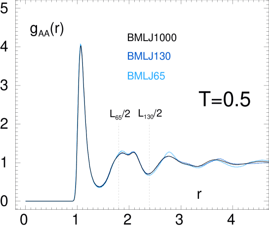
Figure 1: Pair-correlation function, $g_{AA}(r)$, between $A$ particles, for $N=1000,130,$ and 65. Periodic images of the simulation box have been used to compute $g_{AA}(r)$ for distances larger than half the box width, $r>L_{N}/2$ ($N=130$ and $65$).

Within a simulation box of width $L_{N}$, we may only calculate $g_{\alpha\beta}(r)$ for $r<L_{N}/2$. For larger values of $r$, periodic images of the simulation box must be used. We find that $g_{AA}(r)$ of the BMLJ65 is identical to the one of the BMLJ1000 for $r<L_{65}/2$. At larger distances, deviations from the bulk distribution can be seen. This is plausible, since the simple duplication of the simulation box can surely not reproduce all details of the long-ranged bulk correlations. Nevertheless, the oscillations corresponding to higher-order neighbor shells in the BMLJ1000 are also present in the duplicated BMLJ65. Similarly, the BMLJ130 matches the BMLJ1000 $g_{AA}(r)$ for $r<L_{130}/2$, whereas deviations for larger $r$ already seem to be negligibly small.

Statistics of minima.

It is an important question how the properties of the PEL are affected by changes in system size. The most prominent characteristics of a PEL minimum are its energy $\epsilon$ and vibrational partition function $T^{(3N-3)/2}Y$. The latter can be calculated within harmonic approximation,

$$Y=\prod_{\nu}\left({\frac{2\pi}{\lambda_{\nu}}}\right)^{1/2},$$ (1)

where the $\lambda_{\nu}$ are the eigenvalues of the hessian matrix in the minimum. Since the number of PEL minima is extremely large, a statistical treatment is needed. As a starting point, we analyze the mean energy of minima at temperature $T$, $\left\langle{\epsilon(T;N)}\right\rangle$, and their variance $\sigma^{2}(T;N)$. For systems composed of independent subsystems, $\left\langle{\epsilon(T;N)/N}\right\rangle$ and $\sigma^{2}(T;N)/N$ do not depend on system size.

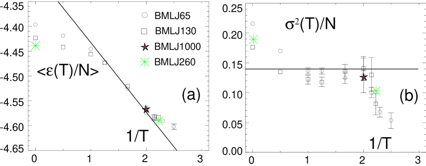
Figure 2: (a) Mean minimum energy per particle vs. $1/T$. Data of different system sizes are given. (b) Variance of minimum energies, also on a per-particle base, again vs. $1/T$. In (a) and (b), the straight lines are the predictions from a gaussian density of minima. At $1/T=0$, minimizations were performed from configurations with random particle positions.

In figure 2, these quantities are shown for $N=65$ and $N=130$, plus some data points of $N=260$ and $N=1000$. Concerning the mean energies, we find a good overall agreement of different system sizes. The maximum difference is about $1\%$ between the BMLJ65 and the BMLJ260 at $T=\infty$. In the landscape-influenced regime below $T=2T_{c}$, data for different $N$ show a perfect match. A similar conclusion can be drawn from figure 2(b), where we see $\sigma^{2}(T)/N$. A systematically larger value is found for the BMLJ65 at high temperatures, as compared to the BMLJ130. For $T\leq 2T_{c}$, the difference is less than $20\%$, but more precise statements are prohibited by the statistical uncertainty of $\sigma^{2}(T)/N$ below $T=0.6$. Thus, small but significant finite-size effects can be observed in this quantity.

We shortly comment on the deviations from the gaussian prediction at $T<0.5$, as seen in figure 2(a),(b). A possible explanation is that our simulations below $T=0.5$ were too short to sample the PEL thoroughly at the lowest energies. In view of the total simulation times for the BMLJ65 ($T=0.4$: $50\tau_{\alpha}$, $T=0.435$: $520\tau_{\alpha}$, $T=0.45$: $850\tau_{\alpha}$) this is strong statement. We currently study if significantly longer simulations could alter the situation in figure 2, $T<0.5$.

Total number of minima.

The overall statistics of PEL minima can be described to a large degree by the number density of their energies, $G(\epsilon)$. Formally, it can be written as $G(\epsilon)=\sum_{i}\delta(\epsilon-\epsilon_{i})$, whereas in practice, some coarse graining of energy is introduced. In computer simulations, $G(\epsilon)$ was found to be approximately gaussian for several model systems Büchner and Heuer (1999); Sciortino et al. (2000); Starr et al. (2001); La Nave et al. (2002),

$$G(\epsilon)=\frac{1}{\sqrt{2\pi\sigma^{2}}}\exp\left({\alpha N-\frac{1}{2\sigma^{2}}(\epsilon-\epsilon_{0})^{2}}\right),\quad\quad\epsilon>\epsilon_{\textrm{\tiny{min}}}.$$ (2)

The lower cutoff energy $\epsilon_{\textrm{\tiny{min}}}$ takes into account that the ideal gaussian cannot extend to arbitrarily low energies. A cutoff at the high-energetic tail of $G(\epsilon)$ is not needed, due to the small Boltzmann weight of these minima. For huge systems, which, to a good approximation, are composed of many independent subsystems, the gaussianity of $G(\epsilon)$ is an immediate consequence of the central limit theorem. However, as discussed in reference Heuer and Büchner (2000), a large degree of gaussianity must already be present in the subsystems that are considered elementary.

The modification of the gaussian by the cutoff $\epsilon_{\textrm{\tiny{min}}}$ is normally small, so that one finds $N_{0}(N)\equiv\int{\rm d}\epsilon G(\epsilon)\approx e^{\alpha N}$. Thus, the so-called growth parameter $\alpha$ describes how the total number of minima, $N_{0}(N)$, evolves with system size. We will now calculate $N_{0}(65)$ and $N_{0}(130)$. To this end, we apply a practical method which has recently been discussed in the literature Sciortino et al. (1999); Mossa et al. (2002b); Sastry (2001); Scala et al. (2000); Sastry (2000). The main step is to compute the partition function $Z(T)$ or, equivalently, the entropy via thermodynamic integration from a known reference state. The knowledge of $Z(T)$ can be used to compute $G(\epsilon)$ as follows Sastry (2000). Using the harmonic approximation of basin vibrations, the population of minimum $i$ at temperature $T$ is

$$p_{i}=\frac{1}{Z(T)}T^{(3N-3)/2}Y_{i}e^{-\beta\epsilon_{i}},$$ (3)

where $\beta=1/k_{\rm B}T$. By computing the expectation value $\sum_{i}Y_{i}^{-1}e^{\beta\epsilon_{i}}\delta(\epsilon-\epsilon_{i})p_{i}$, we can then extract $G(\epsilon)$,

$$\ln G(\epsilon^{\prime})=\ln\left\langle{\delta(\epsilon-\epsilon^{\prime})Y^{-1}e^{\beta\epsilon}}\right\rangle+\ln Z(T)-\frac{3N-3}{2}\ln T.$$ (4)

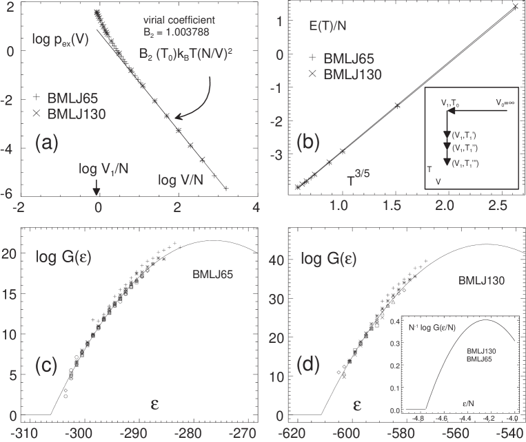
Figure 3: Determination of $G(\epsilon)$ via thermodynamic integration. (a) Excess pressure $p_{\textrm{\tiny{ex}}}=p-Nk_{\rm B}T/V$ over $V/N$ in a double-logarithmic plot. The straight line corresponds to the first correction to ideal-gas behavior, described by the second virial coefficient $B_{2}(T)$. (b) Temperature dependence of the mean potential energy $E(T)/N\equiv\left\langle{V(x)}\right\rangle/N$. Lines are fits of the form $E(T)=a+bT^{3/5}$. Note that the data of BMLJ65 and BMLJ130 practically coincide. Inset: thermodynamic integration path in the $V-T$ plane ($T_{0}=5.0$, $N/V_{1}=1.2$). (c) Number density of minimum energies, $G(\epsilon)$, computed via equation 4 from simulation runs of the BMLJ65 at $T=0.4,0.435,0.45,0.466,0.48,0.5,$ and $0.6$. (d) Number density $G(\epsilon)$ of the BMLJ130, computed from $T=0.4,0.435,0.45,0.5,$ and $0.6$. In (c) and (d), data for $T\geq 0.8$ ($+$) do not fall onto the master curve, indicating the beginning breakdown of the harmonic approximation. Inset: number density of minima of BMLJ65 and BMLJ130, on a per-particle base. Curves coincide completely.

In the above cited works, starting from a high-temperature ($T_{0}$), low-density state ($N/V_{0}$), one compressed the system until the required volume $V_{1}$ of the supercooled liquid was reached. Subsequently, one cooled along the isochore down to $T=T_{1}$. The procedure is depicted in figure 3(b),inset. The partition function at the state point $(V_{1},T_{1})$ follows with the help of the relations

$$\left({\frac{\partial\ln Z}{\partial V}}\right)_{T}=\beta p(V,T),\quad\textrm{ and }\quad\left({\frac{\partial\ln Z}{\partial\beta}}\right)_{V}=-E(V,T),$$

$$\ln Z(V_{1},T_{1})=\ln Z(V_{0},T_{0})+\beta_{0}\int\limits_{V_{0}}^{V_{1}}{\rm d}Vp(V,T_{0})-\int\limits_{\beta_{0}}^{\beta_{1}}{\rm d}\beta E(V_{1},T).$$ (5)

In the limit $V_{0}\to\infty$, we may replace $\ln Z(V_{0},T_{0})$ in equation 5 by the ideal gas term. Note that we write $E(V,T)$ instead of $\left\langle{V}\right\rangle$ for potential energy here, in order to avoid confusion with volume.

After measuring the pressure-volume dependence at $T_{0}=5$ (see figure 3(a)), we evaluate the first integral of equation 5. This yields the partition function at $T_{0}=5$, $\rho_{1}=1.2$,

$$\ln Z(V_{1},T_{0}) =-108.3\pm 0.7\quad\quad\textrm{(BMLJ65)},$$ (6)

$$\ln Z(V_{1},T_{0}) =-218.5\pm 2.5\quad\quad\textrm{(BMLJ130)}.$$ (7)

Considering the second integral of equation 5, we need the mean potential energy $E(T)$ along the isochore $V=V_{1}$ (see figure 3(b)). As is done in the literature, we use the functional form $E(T)=a+bT^{3/5}$ to parametrize our data. For the theoretical background of this form, see reference Rosenfeld and Tarazona (1998). From the two fit parameters

$$a=-361.4\pm 0.3, \quad b=171.5\pm 0.3\quad\quad\textrm{(BMLJ65)},$$ (8)

$$a=-718.8\pm 0.8, \quad b=341.2\pm 0.9\quad\quad\textrm{(BMLJ130)},$$ (9)

one can then calculate the second integral in equation 5.

We now use these results to calculate $N_{0}$, via equation 4. The expectation value in equation 4 is extracted from regular simulations. Thus, as long as the harmonic approximation holds, we are able to calculate the absolute value of $G(\epsilon)$. For the BMLJ65 and BMLJ130 systems, $G(\epsilon)$ is shown in figure 3(c) and (d), respectively. At temperatures $T\leq 0.6$, all points for $G(\epsilon)$ fall nicely onto a master curve, whereas for $T\geq 0.8$ the normalization does not work anymore, see reference Sastry (2000). We then fit gaussians to the data at $T\leq 0.6$, yielding the complete $G(\epsilon)$. The number of minima can now be calculated from $N_{0}=\int{\rm d}\epsilon G(\epsilon)$,

$$N_{0} =10^{22.4\pm 0.8}\quad\quad\textrm{(BMLJ65)},$$ (10)

$$N_{0} =10^{45.0\pm 2.5}\quad\quad\textrm{(BMLJ130)}.$$ (11)

Hence, within error bars, we find $N_{0}(130)=(N_{0}(65))^{2}$, which is the trivial scaling behavior expected from combinations of non-interacting subsystems.

We finally note that we reached the same conclusion after calculating the configurational entropy $S_{c}(T;N)$ as described in reference Sciortino et al. (1999) (data not shown here): $S_{c}(T;N)/N$ turns out to be identical for $N=65$ and $N=130$.

III Dynamic properties.

We now discuss the influence of system size on dynamics. Here, more drastic effects than in static quantities are to be expected: In fact, it is the most puzzling feature of the glass transition itself that a dramatic slowdown of molecular motion cannot be traced back to changes in static quantities easily.

Diffusion coefficients.

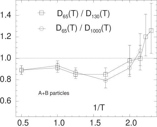
Figure 4: Ratios of diffusion coefficients $D_{N}(T)$ for three system sizes versus $1/T$.

We start with the long-time diffusion coefficient $D_{N}(T)$, defined by the Einstein relation. One finds that the $D_{N}(T)$ for $N=65,130$, and $1000$ differ only very little. In figure 4, we see $D_{65}/D_{1000}$ and $D_{65}/D_{130}$ as functions of temperature. The difference between $D_{65}$ and $D_{1000}$ -which we assume to be identical to the bulk diffusion coefficient- is twenty percent or less above $T_{c}$. Since data for $D_{1000}$ are not available below $T_{c}$, no such comparison is possible there. As reflected by $D_{65}/D_{130}$, these differences are already present between $N=65$ and $N=130$. Below $T_{c}$, however, the BMLJ65 seems to become slightly faster than the BMLJ130. However, since error bars are large for the two low-temperature data points, it is hard to judge whether this is a systematic effect that further increases upon cooling. In any event, in the temperature range studied, the overall variation of $D_{N}(T)$ is more than three orders of magnitude. Regarding the small deviation of the BMLJ65 relative to the BMLJ1000, finite-size effects in the long-time diffusion should be jugded small. As a comparison, major changes happen when going to $N=40$, where we find $D_{40}(0.5)/D_{1000}(0.5)\approx 0.1$.

Waiting-time distributions.

As a more refined comparison of dynamics between different system sizes, we consider the distributions of MB lifetimes (waiting times), see references Doliwa and Heuer (2002a); Denny et al. (2002). A detailed description of MBs and their properties can be found in reference Doliwa and Heuer (2002b). Here we briefly describe how MB lifetimes can be obtained from a given simulation run. Based on an equidistant time series of minima, we resolve the elementary transitions between minima by further minimizations, accompanied by temporal interval bisection. From the series of configurations thus obtained, we determine the time intervals of correlated back-and-forth jumps within groups of a few minima, which are identified with the MB lifetimes Büchner and Heuer (2000); Doliwa and Heuer (2002b). In this way, we are able to detect MB durations ranging from one MD step to many millions of them. At some arbitrary time of a simulation run, the probability to be in a MB of length $\tau$ is $p(\tau)=\sum_{i}\tau_{i}\delta(\tau-\tau_{i})/\sum_{i}\tau_{i}$, where the $\tau_{i}$’s are the lifetimes found in the run. (Since the MB residence times span more than six orders of magnitude, our numerical computations will involve the distributions $p(\log\tau)=p(\tau)\tau\ln 10$ rather than $p(\tau)$.) The temperature dependence of $p(\tau)$ will be suppressed for notational convenience.

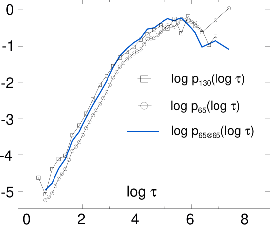
Figure 5: Distributions of MB lifetimes, $p(\log\tau)$ at $T=0.5$. As discussed in the text, the distribution $p_{130}(\log\tau)$ should be reproducable from $p_{65}(\log\tau)$ by a special kind of convolution, equation 12. The corresponding function $p_{65\otimes 65}(\log\tau)$ is given in the figure.

Guided by the idea that a BMLJ130 system is basically a duplication of two independent BMLJ65s, we may ask whether the distribution $p_{130}(\tau)$ of the larger system can be reproduced by some sort of convolution of the distribution $p_{65}(\tau)$ of the smaller one. (For a combined system, MB lifetimes are defined as the periods where neither of the subsystems relaxes.) Indeed, after a lengthy calculation one finds for the duplicated system,

$$p_{65\otimes 65}(\tau)=-\frac{{\rm d}}{{\rm d}\tau}\int\limits_{\tau}^{\infty}{\rm d}{\tau^{\prime}}p_{65}(\tau^{\prime})\int\limits_{\tau}^{\infty}{\rm d}{\tau^{\prime\prime}}p_{65}(\tau^{\prime\prime})\left({1-\frac{\tau^{2}}{\tau^{\prime}\tau^{\prime\prime}}}\right).$$ (12)

This expression can be simplified and, upon using $p(\log\tau)$, it reads

$$p_{65\otimes 65}(\log\tau)=2p_{65}(\log\tau)I(\tau)+2\tau\tilde{I}(\tau)\left({\tilde{I}(\tau)\tau\ln 10-p_{65}(\log\tau)}\right),$$ (13)

where

$$I(\tau)=\int\limits_{\tau}^{\infty}{\rm d}{\tau^{\prime}}p(\tau^{\prime})\quad\textrm{ and }\quad\tilde{I}(\tau)=\int\limits_{\tau}^{\infty}{\rm d}{\tau^{\prime}}p(\tau^{\prime})/\tau^{\prime}.$$

In figure 6, we show $p_{65}(\log\tau)$, together with $p_{130}(\log\tau)$ at the temperature $T=0.5$. The distribution resulting from the duplication, $p_{65\otimes 65}(\log\tau)$, is also given in the figure. It agrees nicely with $p_{130}$. Thus, on the refined level of waiting-time distributions, we find further evidence that larger systems basically behave as consisting of non-interacting BMLJ65-type building blocks. Essentially, $p_{130}$ is shifted to the left with respect to $p_{65}$. This is no wonder, because time intervals where both independent systems are inert, are generally shorter than the waiting times of a single system. For instance, the mean waiting times obey the relation

$$\left\langle{\tau}\right\rangle_{65}=2\left\langle{\tau}\right\rangle_{65\otimes 65},$$

which can be shown with the help of equation 12.

Metabasin depths.

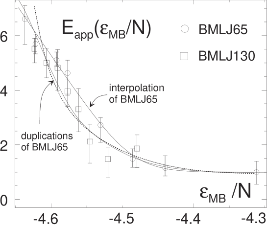
Figure 6: Apparent activation energies $E_{\textrm{\tiny{app}}}(\epsilon_{\textrm{\tiny{MB}}}/N)$ derived from mean lifetimes at fixed metabasin energy $\epsilon_{\textrm{\tiny{MB}}}$ (equation 14). Data for $N=65$ and $N=130$ are shown versus $\epsilon_{\textrm{\tiny{MB}}}/N$. The interpolation of the $N=65$ data has been used to compute $E_{\textrm{\tiny{app}}}$ for the union of two non-interacting BMLJ65, as described in the text. The result of this calculation is given in the figure (solid line). Three further duplications yield $E_{\textrm{\tiny{app}}}$ for $N=1040$ (dashed line).

As discussed above, metabasins have turned out as the relevant structures in the PEL for describing the slowdown of molecular motion in supercooled liquids. In a recent paper, we reported on how the average lifetimes $\left\langle{\tau|\epsilon_{\textrm{\tiny{MB}}};T}\right\rangle$ of MBs depend on their energies $\epsilon_{\textrm{\tiny{MB}}}$ Doliwa and Heuer (2002b). At some fixed $\epsilon_{\textrm{\tiny{MB}}}$, we found that $\left\langle{\tau|\epsilon_{\textrm{\tiny{MB}}};T}\right\rangle$ is Arrhenius-like below $T\approx 2T_{c}$, leading to the parametrization

$$\left\langle{\tau|\epsilon_{\textrm{\tiny{MB}}};T}\right\rangle=\tau_{0}(\epsilon_{\textrm{\tiny{MB}}})e^{\beta E_{\textrm{\tiny{app}}}(\epsilon_{\textrm{\tiny{MB}}})}.$$ (14)

The apparent activation energy $E_{\textrm{\tiny{app}}}(\epsilon_{\textrm{\tiny{MB}}})$ shows a strong dependence on $\epsilon_{\textrm{\tiny{MB}}}$, as soon as one drops below $\epsilon_{\textrm{\tiny{MB}}}/N\approx-4.5$. This can be seen in figure 6 where $E_{\textrm{\tiny{app}}}(\epsilon_{\textrm{\tiny{MB}}})$ versus $\epsilon_{\textrm{\tiny{MB}}}/N$ is depicted both for $N=65$ and $N=130$. Naturally, it is tempting to relate $E_{\textrm{\tiny{app}}}(\epsilon_{\textrm{\tiny{MB}}})$ to PEL structure. By a detailed investigation of escape paths and the barriers that are overcome when escaping the MBs, we were able to reproduce $E_{\textrm{\tiny{app}}}(\epsilon)$ from the local topology of MBs. Hence, we were able to prove that the effective depth $E_{\textrm{\tiny{app}}}$ of a MB, derived from dynamics, directly corresponds to the real depth of that MB as given by the energy barriers around it. Moreover, escaping from deep MBs could be shown to involve actived jumps even above $T_{c}$. What concerns the prefactor $\tau_{0}(\epsilon_{\textrm{\tiny{MB}}})$ of equation 14, no such understanding in terms of PEL structure has been possible. Fortunately, however, $\tau_{0}(\epsilon_{\textrm{\tiny{MB}}})$ turned out to have a weak dependence on MB energy. Thus, it may in good conscience be set to a constant Doliwa and Heuer (2002b).

Here we concentrate on the dependence of $E_{\textrm{\tiny{app}}}(\epsilon_{\textrm{\tiny{MB}}})$ on system size. As can be seen from figure 6, the activation energies $E_{\textrm{\tiny{app}}}(\epsilon_{\textrm{\tiny{MB}}}/N)$ of $N=65$ and $N=130$ are quite close. However, the $N=130$ data for $\epsilon_{\textrm{\tiny{MB}}}/N<-4.5$ show the tendency to fall slightly below that of $N=65$. We shall show that this trend can be understood again in terms of a simple duplication of a BMLJ65. Hence, we are interested in the combination of two independent BMLJ65 systems. Consider a MB of energy $\epsilon_{\textrm{\tiny{MB}}}=\epsilon_{\textrm{\tiny{MB}}}^{\textrm{\tiny{(1)}}}+\epsilon_{\textrm{\tiny{MB}}}^{\textrm{\tiny{(2)}}}$ in the combined system. Then assume that its average lifetime can be expressed through the lifetimes of both subsystems, i.e.

$$\frac{1}{\left\langle{\tau|\epsilon_{\textrm{\tiny{MB}}}^{\textrm{\tiny{(1)}}},\epsilon_{\textrm{\tiny{MB}}}^{\textrm{\tiny{(2)}}}}\right\rangle_{65\otimes 65}}=\frac{1}{\left\langle{\tau|\epsilon_{\textrm{\tiny{MB}}}^{\textrm{\tiny{(1)}}}}\right\rangle_{65}}+\frac{1}{\left\langle{\tau|\epsilon_{\textrm{\tiny{MB}}}^{\textrm{\tiny{(2)}}}}\right\rangle_{65}}.$$ (15)

Averaging over the population of $\epsilon_{\textrm{\tiny{MB}}}^{\textrm{\tiny{(1)}}}$ and $\epsilon_{\textrm{\tiny{MB}}}^{\textrm{\tiny{(2)}}}$ at constant $\epsilon_{\textrm{\tiny{MB}}}$ then yields $\left\langle{\tau|\epsilon_{\textrm{\tiny{MB}}};T}\right\rangle$ for the combined system. The mean lifetimes produced in this way are again Arrhenius-like below $2T_{c}$ (data not shown here). Thus, data can again be fitted by a function of the form of equation 14, yielding $E_{\textrm{\tiny{app}}}(\epsilon_{\textrm{\tiny{MB}}})$ for the duplicated BMLJ65. The result is shown in figure 6 for $T=0.5$. Again, the artificial BMLJ65 duplication reproduces the observations for the real system of $N=130$ particles.

Finally, we note that further duplication of the BMLJ65 leads to an interesting result: The activation energies from duplication nearly fall on top of each other for $N\geq 130$ and $\epsilon_{\textrm{\tiny{MB}}}/N>-4.6$. The example of sixteen non-interacting BMLJ65s ($N=1040$) is shown in figure 6.

IV Discussion and Conclusions.

For several static and dynamic observables, we have verified the factorization property

$$\textrm{ BMLJ130 }\approx\textrm{ BMLJ65 }\otimes\textrm{ BMLJ65 }.$$

The BMLJ130, in turn, seems to be close to bulk behavior. Some of the results presented here have already been obtained in earlier work for a very similar Lennard-Jones type system Büchner and Heuer (1999). Again, the conclusion can be drawn that binary Lennard-Jones systems of ca. 60 particles are a very good compromise between the desired smallness needed for our PEL investigations and the required absence of large finite-size related artifacts. In this connection, the simulation results of Yamamoto and Kim on the standard binary soft sphere mixture are of interest Kim and Yamamoto (2000). Comparing systems of $N=108$ and $1000$ particles above $T_{c}$, the authors found the small system to be up to an order of magnitude slower than the large one. These findings suggest a fundamental difference between the Lennard-Jones and soft-sphere types of relaxation dynamics. Evidently, soft spheres exibit a larger length scale of cooperative motion than do Lennard-Jones systems. A possible explanation can be found in reference Büchner and Heuer (1999).

It is known from the study of cooperative length scales that they increase with decreasing temperature Donati et al. (1999); Bennemann et al. (1999); Doliwa and Heuer (2000). Thus, at some lower temperatures one might expect that 65 particles are no longer enough and finite-size effects become visible. For a similar Lennard-Jones system it has been shown that finite-size effects are reflected by the fact that the bottom of the PEL is frequently probed Büchner and Heuer (1999). In the present case still longer simulations at lower temperatures have to be performed to check whether also for $N=65$ the PEL bottom can be reached. Then the interesting question arises whether or not differences to the $N=130$ system become visible.

The results presented in this paper suggest that the essential physics of the supercooled BMLJ is already contained in the system of $N=65$ particles. For the temperatures under investigation here, extended structures of collectively moving particles (’strings’) have been reported in large systems Donati et al. (1998). It is important to know whether these structures are still present in the small systems considered here. Work along this line is in progress.

References.

References

- Debenedetti and Stillinger (2001) P. G. Debenedetti and F. H. Stillinger, Nature 410, 259 (2001).
- Goldstein (1969) M. Goldstein, J. Chem. Phys. 51, 3728 (1969).
- Stillinger (1995) F. H. Stillinger, Science 267, 1935 (1995).
- Stillinger and Weber (1982) F. H. Stillinger and T. A. Weber, Phys. Rev. A 25, 978 (1982).
- Mossa et al. (2002a) S. Mossa, E. La Nave, P. Tartaglia, and F. Sciortino, e-print cond-mat/0209181 (2002a).
- Götze and Sjogren (1992) W. Götze and L. Sjogren, Rep. Prog. Phys. 55, 241 (1992).
- Angelani et al. (2000) L. Angelani, R. D. Leonardo, G. Ruocco, A. Scala, and F. Sciortino, Phys. Rev. Lett. 85, 5356 (2000).
- Broderix et al. (2000) K. Broderix, K. K. Bhattacharya, A. Cavagna, A. Zippelius, and I. Giardina, Phys. Rev. Lett. 85, 5360 (2000).
- Doliwa and Heuer (2002a) B. Doliwa and A. Heuer, e-print cond-mat/0205283 (2002a).
- Doliwa and Heuer (2002b) B. Doliwa and A. Heuer, e-print cond-mat/0209139 (2002b).
- Büchner and Heuer (2000) S. Büchner and A. Heuer, Phys. Rev. Lett. 84, 2168 (2000).
- Büchner and Heuer (1999) S. Büchner and A. Heuer, Phys. Rev. E 60, 6507 (1999).
- Sciortino et al. (2000) F. Sciortino, W. Kob, and P. Tartaglia, J. Phys.-Condes. Matter 12, 6525 (2000).
- Starr et al. (2001) F. W. Starr, S. Sastry, E. La Nave, A. Scala, H. E. Stanley, and F. Sciortino, Phys. Rev. E 6304, 041201 (2001).
- La Nave et al. (2002) E. La Nave, S. Mossa, and F. Sciortino, Phys. Rev. Lett. 88, 225701 (2002).
- Heuer and Büchner (2000) A. Heuer and S. Büchner, J. Phys.-Condes. Matter 12, 6535 (2000).
- Sciortino et al. (1999) F. Sciortino, W. Kob, and P. Tartaglia, Phys. Rev. Lett. 83, 3214 (1999).
- Mossa et al. (2002b) S. Mossa, E. La Nave, H. E. Stanley, C. Donati, F. Sciortino, and P. Tartaglia, Phys. Rev. E 65, 041205 (2002b).
- Sastry (2001) S. Sastry, Nature 409, 164 (2001).
- Scala et al. (2000) A. Scala, F. W. Starr, E. La Nave, F. Sciortino, and H. E. Stanley, Nature 406, 166 (2000).
- Sastry (2000) S. Sastry, J. Phys.-Condes. Matter 12, 6515 (2000).
- Rosenfeld and Tarazona (1998) Y. Rosenfeld and P. Tarazona, Mol. Phys. 95, 141 (1998).
- Denny et al. (2002) R. A. Denny, D. R. Reichman, and J.-P. Bouchaud, e-print cond-mat/0209020 (2002).
- Kim and Yamamoto (2000) K. Kim and R. Yamamoto, Phys. Rev. E 61, R44 (2000).
- Donati et al. (1999) C. Donati, S. C. Glotzer, and P. H. Poole, Phys. Rev. Lett. 82, 5064 (1999).
- Bennemann et al. (1999) C. Bennemann, C. Donati, J. Baschnagel, and S. C. Glotzer, Nature 399, 246 (1999).
- Doliwa and Heuer (2000) B. Doliwa and A. Heuer, Phys. Rev. E 61, 6898 (2000).
- Donati et al. (1998) C. Donati, J. F. Douglas, W. Kob, S. J. Plimpton, P. H. Poole, and S. C. Glotzer, Phys. Rev. Lett. 80, 2338 (1998).