Anomalous diffusion in nonlinear oscillators with multiplicative noise

Abstract

The time-asymptotic behavior of undamped, nonlinear oscillators with a random frequency is investigated analytically and numerically. We find that averaged quantities of physical interest, such as the oscillator’s mechanical energy, root-mean-square position and velocity, grow algebraically with time. The scaling exponents and associated generalized diffusion constants are calculated when the oscillator’s potential energy grows as a power of its position: ${\mathcal{U}}(x)\sim x^{2n}$ for $|x|\rightarrow\infty$. Correlated noise yields anomalous diffusion exponents equal to half the value found for white noise.

I Introduction

Randomness in the external conditions entails the parameters of a dynamical system to fluctuate. The extent of these fluctuations is independent of any thermodynamic characteristic of the system in contrast to intrinsic fluctuations the amplitude of which is proportional to the equilibrium temperature, in accordance with the fluctuation-dissipation theorem vankampen ; risken . Usually, external randomness appears as a multiplicative noise in the dynamical equations. The interplay of noise and nonlinearity in a system far from equilibrium results in some unusual phenomena lefever . In fact, the presence of noise dramatically alters the properties of a nonlinear dynamical system both qualitatively and quantitatively (for a recent review see landaMc ). For example, it was shown recently that in a spatially-extended system, a multiplicative noise, white in space and time, generates an ordered symmetry-breaking state through a non-equilibrium phase transition whereas no such transition exists in the absence of noise vandenb1 ; vandenb2 . Noise can also induce spatial patterns vandenb3 ; toral or improve the performance of a nonlinear device through stochastic resonance barbay . Furthermore, even if some important qualitative features of a deterministic system survive to external noise, their quantitative characteristics may change: a stable fixed point may become unstable bourret , a bifurcation may be delayed (noise-induced stabilization) lucke ; roder and scale-invariant properties which manifest themselves as power-laws may be altered with the appearance of non-classical scaling exponents genovese .

The discovery of Brownian motors which are able to rectify random fluctuations into a directed motion (noise-induced transport) has triggered a renewed interest in the study of simple one-dimensional mechanical models of particles in a potential with random parameters reimann . It is well known that a linear oscillator submitted to parametric noise can be unstable even if damping is taken into account bourret ; linden . This noise-induced energetic instability has been observed in diverse experimental contexts such as electronic oscillators strato ; kabashima , nematic liquid crystals kawakubo and surface waves (Faraday instability) fauve . In engineering fields this instability plays a crucial role in the study of the dynamic response of flexible structures to random environmental loading such as the wave-induced motion of off-shore structures or the vibration of tall buildings in a turbulent wind roberts . The presence of nonlinear friction tends to limit the oscillation amplitude: the pendulum with randomly vibrating suspension axis and undergoing nonlinear friction, known as the van der Pol oscillator, has been studied in the small noise limit using perturbative expansions strato ; landa .

In the present work, we consider the motion of an undamped nonlinear oscillator trapped in a general confining potential and submitted to parametric random fluctuations. Because there is no dissipation, the energy of the system increases with time and we shall show that the position, the momentum and the energy grow as power-laws of time with nontrivial exponents that depend on the behavior of the confining potential at infinity bouchaud . A key feature of our method is to use the integrability properties of the associated deterministic nonlinear oscillator in order to derive exact stochastic equations in action-angle variables. We then use the averaging technique of classical mechanics landau , together with a reduction procedure vandenbroeck1 ; drolet , to calculate exactly the anomalous scaling exponents, irrespective of the amplitude of the noise. Some of our results were derived before in the particular case of a cubic nonlinearity using an energy-enveloppe equation lind2 . Our method enables us to derive the numerical prefactors appearing in the scaling laws (generalized diffusion constants), and our analytical predictions compare very satisfactorily with the numerical results. In the case of noise correlated in time, the anomalous diffusion exponents are modified: they can be obtained by dimensional analysis arguments and the values thus found also agree with numerical results. Throughout this work, crossover phenomena between different scaling regimes are emphasized.

This article is organized as follows. In section II, we recall that the energy of a linear oscillator with multiplicative noise grows exponentially with time and that this growth may be characterized by a Lyapunov exponent. In section III, we analyze the classical Duffing oscillator in presence of parametric noise. Our technique allows us to study precisely the long-time behavior of the system. In section IV, we consider a particle in an arbitrary confining potential that grows as a polynomial at large distances. In section V, we discuss the case of colored noise where the presence of a new timescale (the correlation time) leads to a nontrivial crossover from the white noise regime to another scaling regime. Our conclusions are presented in section VI. In Appendix A, the nonlinear oscillator in presence of both additive and multiplicative noise is briefly studied: we show that at long times the effect of additive noise is irrelevant. Appendix B is devoted to numerical methods and in Appendix C some useful mathematical relations are recalled.

II The linear oscillator with parametric noise

In this section we recall known results for an undamped linear oscillator submitted to parametric noise, a generic and widely studied model, in order to understand the role of external multiplicative noise lefever ; bourret ; strato . The dynamical equation for such a system is

$$\frac{\textrm{d}^{2}}{\textrm{d}t^{2}}x(t)+(\omega^{2}+\xi(t))\,x(t)=0,$$ (1)

where $x(t)$ represents the position of the oscillator at time $t$ and $\omega$ its frequency. The random noise $\xi(t)$ is a Gaussian white noise of zero mean-value and of amplitude ${\mathcal{D}}$:

$$\langle\xi(t)\rangle = 0\,,$$

$$\langle\xi(t)\xi(t^{\prime})\rangle = {\mathcal{D}}\,\delta(t-t^{\prime}).$$ (2)

The physical interpretation of Eq. (1) is that the frequency of the oscillator is not constant in time but fluctuates around its mean value $\omega$ because of randomness in the external conditions (external noise). When these fluctuations are deterministic and periodic in time, Eq. (1) is a Mathieu equation which has been extensively studied landau . Here, we are interested in the case where these fluctuations are random with no deterministic part. The origin, $x=0$ and $\textrm{d}x/\textrm{d}t=0$, is an unstable stationary solution of Eq. (1). As shown in Ref. bourret , this instability can be studied from the dynamical evolution of the Probability Distribution Function $P(x,v,t)$ of $x$ and $v$ (with $v=\dot{x}=\textrm{d}x/\textrm{d}t)$. This P.D.F. obeys the Fokker-Planck equation vankampen ; risken associated with Eq. (1):

$$\frac{\partial P}{\partial t}=-v\frac{\partial P}{\partial x}+\omega^{2}x\frac{\partial P}{\partial v}+\frac{{\mathcal{D}}}{2}\frac{\partial^{2}}{\partial v^{2}}\left(x^{2}P\right),$$ (3)

where Eq. (1) is understood according to Stratonovich rules.

This Fokker-Planck equation leads to a closed system of ordinary differential equations that couple the $n+1$ moments of order $n$, i.e., moments of the type $\langle x^{n-k}v^{k}\rangle$, where $n$ and $k$ are positive integers and $0\leq k\leq n$:

$$\frac{\textrm{d}}{\textrm{d}t}\langle x^{n-k}v^{k}\rangle=(n-k)\,\langle x^{n-k-1}v^{k+1}\rangle-\omega^{2}k\,\langle x^{n-k+1}v^{k-1}\rangle+\frac{\mathcal{D}}{2}\,k(k-1)\,\langle x^{n-k+2}v^{k-2}\rangle.$$ (4)

The divergence of the moments with time results from the existence of at least one positive eigenvalue of the linear system (4). In particular, the mean value of the mechanical energy $E$ of the system (i.e. the sum of its kinetic and potential energies) grows exponentially with time:

$$\langle E\rangle=\frac{1}{2}\,\langle v^{2}\rangle+\frac{1}{2}\omega^{2}\,\langle x^{2}\rangle\propto e^{\mu\,t},$$ (5)

where the growth rate $\mu$ is the positive real root of the equation:

$$\mu^{3}+4\omega^{2}\mu=2{\mathcal{D}}.$$ (6)

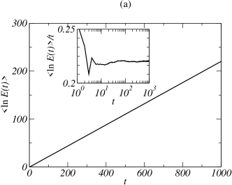
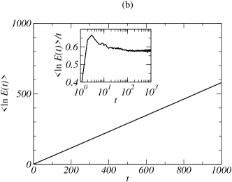
Figure 1: Linear oscillator with multiplicative noise: Eq. (1) is integrated numerically for ${\mathcal{D}}=1$ with a timestep $\delta t=10^{-3}$. Ensemble averages are computed over $10^{4}$ realizations. We plot the average $\langle\ln E(t)\rangle$ and the ratio $\langle\ln E(t)\rangle/t$ (inset) vs. time $t$. Fig. (a): $\omega=1$, $\Lambda(\omega=1)=\lim_{t\rightarrow\infty}\langle\ln E(t)\rangle/t=0.219(3)$; Fig. (b): degenerate case $\omega=0$, $\Lambda(\omega=0)\simeq 0.580(5)$. Both estimates of the Lyapunov exponent are in good agreement with the theoretical prediction hansel ; tessieri .

It has also been proved that the quenched average of the energy $E$ grows linearly with time, hence the Lyapunov exponent $\Lambda$, defined as

$$\Lambda=\lim_{t\rightarrow\infty}\frac{1}{t}\,\langle\log E\rangle,$$ (7)

is finite and strictly positive hansel ; tessieri . The positivity of the Lyapunov exponent implies the instability of all moments at long times. Note that the growth rate $\mu$, defined in Eq. (5), is larger than the Lyapunov exponent because of the convexity inequality, $\log\langle E\rangle\geq\langle\log E\rangle$.

In Figure 1(a), we present the numerical solution of Eq. (1) averaged over a large number of realizations of the noise, where the pulsation is $\omega=1$. The algorithm used to solve this stochastic differential equation with multiplicative noise is inspired from mannella and explained in Appendix B. A numerical estimate of the Lyapunov exponent, given in Fig. 1(a), agrees very well with the analytic expression of Refs. hansel ; tessieri . The usual statistical equipartition of the total energy between kinetic and potential contributions is satisfied: $\langle E\rangle=\omega^{2}\,\langle x^{2}\rangle=\langle v^{2}\rangle$.

In Figure 1(b), we show the same quantities for the degenerate linear oscillator obtained by taking $\omega$ equal to 0. This degenerate case exhibits the same behavior as the generic case and the Lyapunov exponent can be calculated by taking the $\omega\to 0$ limit in the formulas of Refs. hansel ; tessieri . We conclude that the instability triggered by the noise is the dominant effect and that the presence of the linear restoring force $-\omega^{2}x$ is irrelevant.

Hence, in order to avoid an exponential increase of the energy and the amplitude of the oscillator, it is necessary to go beyond the linear approximation and consider the effect of nonlinear restoring forces degli .

III Duffing oscillator with multiplicative noise

We now analyze the effect of a nonlinear restoring force in an oscillator submitted to an external multiplicative noise. In order to preserve the $x\to-x$ symmetry, the nonlinear term has to be odd in the amplitude $x$. In this section, we study the particular case of a cubic nonlinearity

$$\frac{\textrm{d}^{2}}{\textrm{d}t^{2}}x(t)+(\omega^{2}+\xi(t))\,x(t)+\lambda\,x(t)^{3}=0.$$ (8)

The coefficient of the nonlinear term is set equal to unity by rescaling the variable $x(t)$ to $x(t)\,\sqrt{\lambda}$. The random noise $\xi$ is a Gaussian white noise of amplitude ${\mathcal{D}}$ as defined in Eq. (2). The deterministic nonlinear mechanical system correponding to Eq. (8) is known as the Duffing oscillator. We shall prove that the cubic term is relevant and prevents the average amplitude from growing exponentially. Instead of an exponential behavior, the average energy of the oscillator as well as the variances of its position and velocity exhibit a power-law behavior with time. We shall calculate exactly the associated scaling exponents.

III.1 The degenerate cubic oscillator

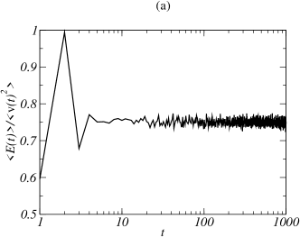
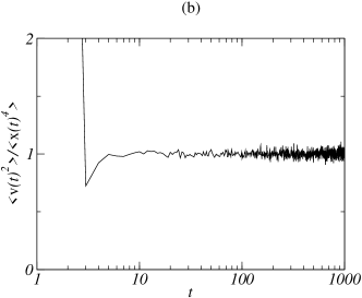
Figure 2: Cubic oscillator: energy equipartition. Eq. (9) is integrated numerically for ${\mathcal{D}}=1$ with a timestep $\delta t=5\,10^{-4}$. Ensemble averages are computed over $10^{4}$ realizations. The ratios $\langle E(t)\rangle/\langle v(t)^{2}\rangle$ and $\langle v(t)^{2}\rangle/\langle x(t)^{4}\rangle$ are approximately constant and respectively equal to $3/4$ and $1$.

The linear part of the restoring force, $-\omega^{2}x$, is negligible in comparison to the cubic term when the amplitude of the oscillator is large. In order to study the long-time behavior of the oscillator, we therefore simplify Eq. (8) to that of a degenerate cubic oscillator:

$$\frac{\textrm{d}^{2}}{\textrm{d}t^{2}}x(t)+\xi(t)\,x(t)+x(t)^{3}=0.$$ (9)

We first study the deterministic part of Eq. (9) and shall add the noise term afterwards roberts . In one dimension, the deterministic cubic oscillator is integrable because the energy $E$ defined as

$$E=\frac{1}{2}\dot{x}^{2}+\frac{1}{4}x^{4},$$ (10)

is a conserved quantity. The exact solution of the mechanical system, $\ddot{x}+x^{3}=0$, for a fixed value of $E$, is given by

$$x = E^{1/4}\,\frac{{\rm sn}\left((4E)^{\frac{1}{4}}t;\frac{1}{\sqrt{2}}\right)}{{\rm dn}\left((4E)^{\frac{1}{4}}t;\frac{1}{\sqrt{2}}\right)},$$ (11)

$$\dot{x} = (2E)^{1/2}\,\frac{{\rm cn}\left((4E)^{\frac{1}{4}}t;\frac{1}{\sqrt{2}}\right)}{{\rm dn}^{2}\left((4E)^{\frac{1}{4}}t;\frac{1}{\sqrt{2}}\right)},$$ (12)

where sn, cn and dn are the classical Jacobi elliptic functions of modulus $1/\sqrt{2}$ abram ; byrd . The properties of elliptic functions that will be useful for our purpose are recalled in Appendix C. From Eqs. (11) and (12), we define the action-angle variables of the cubic oscillator landau ; lichtenberg . The action variable $I$ corresponds to the area under a constant energy curve in phase space:

$$I=4\int_{0}^{(4E)^{\frac{1}{4}}}\sqrt{2E-\frac{x^{4}}{2}}\,\textrm{d}x=8\,\left(\int_{0}^{1}\sqrt{1-u^{4}}\textrm{d}u\right)\,E^{3/4}\propto E^{3/4}.$$ (13)

The angle variable $\phi$, canonically conjugate to the action $I$, is equal to $\omega(E)t$ (but for an unimportant additive constant) where $\omega(E)$ is the frequency corresponding to the energy $E$. From Eqs. (11) and (12), the phase is identified as

$$\phi=(4E)^{\frac{1}{4}}\,t.$$ (14)

This phase variable is defined modulo the common real period $4K$ of the elliptic functions ${\rm sn},{\rm cn},{\rm dn}$ that appear in Eqs. (11) and (12). The quarter of the period is given by

$$K=K(\frac{1}{\sqrt{2}})=\sqrt{2}{\int_{0}^{1}\frac{\textrm{d}u}{\sqrt{1-u^{4}}}}\simeq 1.854\,.$$ (15)

In terms of the energy-angle coordinates $(E,\phi)$, the original variables $(x,\dot{x})$ read as follows:

$$x=E^{1/4}{\rm sd}(\phi;{1}/{\sqrt{2}})\,\,\,\hbox{ and }\,\,\,\dot{x}=(2E)^{1/2}\frac{{\rm cn}(\phi;{1}/{\sqrt{2}})}{{\rm dn}^{2}(\phi;{1}/{\sqrt{2}})},$$ (16)

where we have introduced the function sd = sn/dn. Hence, for the free system (without noise) the second-order dynamical equation, $\ddot{x}+x^{3}=0$, is equivalent to the following two first-order equations, the first one representing energy conservation:

$$\dot{E} = 0\,,$$

$$\dot{\phi} = (4E)^{\frac{1}{4}}\,.$$ (17)

The presence of external noise spoils the integrability of the dynamical system (9) and causes $E$ to grow with time by continuously injecting energy into the system. We now take into account the external noise and rewrite the system (17) in $(E,\phi)$ coordinates. The stochastic evolution equation for the energy is given by

$$\dot{E}=x\dot{x}\xi(t)=\sqrt{2}\,E^{3/4}\,\frac{{\rm sn}(\phi;{1}/{\sqrt{2}})\,{\rm cn}(\phi;{1}/{\sqrt{2}})}{{\rm dn}^{3}(\phi;{1}/{\sqrt{2}})}\,\xi(t)\,.$$ (18)

Inverting the relation (16) between $\phi$ and $x$,

$$\phi={\rm sd}^{-1}\left(\frac{x}{E^{1/4}},\frac{1}{\sqrt{2}}\right)\,,$$ (19)

and using Eqs. (16) and (18), we obtain the stochastic evolution of the phase variable:

$$\dot{\phi}=(4E)^{\frac{1}{4}}-\frac{{\rm sd}^{2}(\phi;{1}/{\sqrt{2}})}{2\sqrt{2}E^{1/4}}\xi(t)\,.$$ (20)

With the help of the auxiliary variable $\Omega$ defined as

$$\Omega=2\sqrt{2}E^{1/4}\,,$$ (21)

we derive a compact and symmetric form for the two stochastic evolution equations (18) and (20):

$$\dot{\Omega} = \frac{{\rm sn}(\phi){\rm cn}(\phi)}{{\rm dn}^{3}(\phi)}\xi(t),$$ (22)

$$\dot{\phi} = \frac{\Omega}{2}-\frac{{\rm sd}^{2}(\phi)}{\Omega}\xi(t).$$ (23)

where the elliptic modulus $1/\sqrt{2}$ common to all the elliptic functions has been omitted. We emphasize that the coupled equations (22) and (23) are mathematically equivalent to the initial system and have been derived without any approximation. Moreover, the nature of the parametric perturbation has played no role in the derivation: the function $\xi(t)$ can be a deterministic or a stochastic function with arbitrary statistical properties.

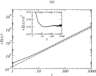
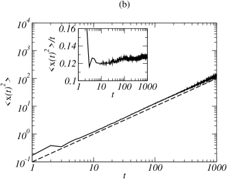
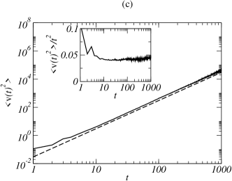
Figure 3: Cubic oscillator: numerical data, obtained for the same runs as in Fig. 2, is represented by solid lines, and compared to the predicted power-law behaviors given by Eqs. (46) (dashed lines). We plot the time-dependence of the following averages: (a) $\langle E(t)\rangle$, (b) $\langle x(t)^{2}\rangle$ and (c) $\langle v(t)^{2}\rangle$. Data plotted in the insets yield the following estimates of the diffusion constants $D_{E}=0.031(1)$, $D_{x}=0.125(5)$, $D_{v}=0.043(3)$, in excellent agreement with theoretical estimates Eqs. (40), (41) and (42).

We now perform a precise analysis of the long-time behavior of the cubic oscillator driven by a multiplicative Gaussian white noise. From a heuristic point of view, we observe from Eq. (22) that $\Omega$ undergoes a diffusion process and should scale typically as $t^{1/2}$. We also notice from Eq. (23) that, as $\Omega$ grows, the phase $\phi$ varies more and more rapidly with time. Hence the phase $\phi$ is a fast variable and it is natural to average the dynamics over its rapid variations. This averaging process leads to some remarkable and general identities between different physical quantitites. Thus, we obtain the average of $\dot{x}^{2}$ from Eq. (16),

$$\langle\dot{x}^{2}\rangle=2\,\overline{\frac{{\rm cn^{2}}(\phi)}{{\rm dn}^{4}(\phi)}}\,\langle E\rangle,$$ (24)

where the overline indicates the mean-value over a period $4K$. The coefficient in Eq. (24) can be calculated explicitly:

$$2\,\overline{\frac{{\rm cn^{2}}(\phi)}{{\rm dn}^{4}(\phi)}}=\frac{4}{3}\,;$$ (25)

the proof of this identity (and of some forthcoming similar identities) is presented in Appendix C. Equation (24) is nothing but a statistical equipartition relation between the mean values of the total energy and kinetic energy:

$$\langle E\rangle=\frac{3}{4}\langle\dot{x}^{2}\rangle.$$ (26)

Such an identity provides a generalization of the usual equipartition theorem valid for quadratic degrees of freedom. Another statistical equality follows from Eq. (26) and the definition (10) of the energy $E:$

$$\langle\dot{x}^{2}\rangle=\langle x^{4}\rangle.$$ (27)

We emphasize that these equalities are ‘universal’ in the sense that they are independent of the form of the noise we consider. The derivation of these equipartition relations relies only on the hypothesis that the distribution of the angle $\phi$ is uniform over the interval $[0,4K]$ when $t\to\infty$. In particular, identities (26) and (27) are valid for multiplicative as well as for additive noise (see Appendix A). Our numerical results (Fig. 2) confirm these relations and that the averaging procedure is therefore valid.

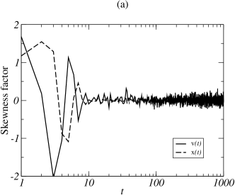
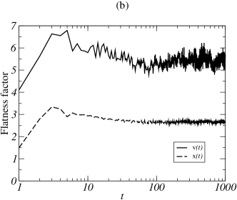
Figure 4: Cubic oscillator. Fig. (a): skewness factors of the position $x(t)$ (dashed line) and velocity $v(t)$ (solid line). Fig. (b): flatness factors of the position $x(t)$ (dashed line) and velocity $v(t)$ (solid line). Numerical data is obtained from the same runs as in Fig. 2.

The same averaging procedure allows us to derive a closed equation for the stochastic evolution of the slow variable $\Omega.$ We start by writing the Fokker-Planck equation governing the evolution of the P.D.F. $P_{t}(\Omega,\phi)$ associated with the system (22,23). Since the noise term appears as a multiplicative factor, one must be cautious about the convention used to define stochastic calculus. Here as well as in the following, we shall use Stratonovich rules because they are obtained naturally when white noise is considered as a limit of colored noise with vanishing correlation time vankampen ; risken . The Fokker-Planck equation corresponding to Eqs. (22) and (23) reads:

$$\partial_{t}P = -\frac{\Omega}{2}\partial_{\phi}P$$ (28)

$$+ \frac{{\mathcal{D}}}{2}\Bigg{(}\partial_{\phi}\left(\frac{g(\phi)}{\Omega}\partial_{\phi}\frac{g(\phi)}{\Omega}P\right)-\partial_{\phi}\left(\frac{g(\phi)}{\Omega}\partial_{\Omega}Pf(\phi)\right)-\partial_{\Omega}\left(f(\phi)\partial_{\phi}\frac{g(\phi)}{\Omega}P\right)+\partial_{\Omega}\left(f(\phi)\partial_{\Omega}f(\phi)P\right)\Bigg{)}\,,$$

where we have defined:

$$f(\phi)=\frac{{\rm sn}(\phi){\rm cn}(\phi)}{{\rm dn}^{3}(\phi)}\,\,\,\hbox{ and }\,\,\,g(\phi)={\rm sd}^{2}(\phi)\,\,.$$ (29)

The Fokker-Planck equation (28) written in the variables $(\Omega,\phi)$ is exact because we study the case of a Gaussian white noise. In order to pursue our calculations, we assume that $P_{t}(\Omega,\phi)$ becomes independent of $\phi$ when $t\to\infty$, i.e., that the probability measure for $\phi$ is uniform over the interval $[0,4K]$. We now average the Fokker-Planck equation (28) over the angular variable. We shall use the fact that the average of the derivative of any function is zero:

$$\overline{\partial_{\phi}(\ldots)}=0\,.$$ (30)

This implies that:

$$\overline{\partial_{\phi}\left(g(\phi)\partial_{\phi}g(\phi)\right)}=0\,\,\,\hbox{ and }\,\,\,\overline{f(\phi)}=0\,\,\,\hbox{ because }\,\,\,f(\phi)=\frac{1}{2}\partial_{\phi}g(\phi)\,.$$ (31)

Using these properties, and in particular the last identity in (31), we derive the phase-averaged Fokker-Planck equation:

$$\partial_{t}\tilde{P}=\frac{{\mathcal{M}}{\mathcal{D}}}{2}\left(\partial_{\Omega}^{2}\tilde{P}-2\partial_{\Omega}\frac{\tilde{P}}{\Omega}\right)\,,$$ (32)

where $\tilde{P}_{t}(\Omega)$ is now a function of $\Omega$ and $t$ only, and where ${\mathcal{M}}$ is given by

$${\mathcal{M}}=\overline{f^{2}(\phi)}=\frac{1}{K}\int_{0}^{K}\frac{{\rm sn^{2}}(\phi){\rm cn^{2}}(\phi)}{{\rm dn}^{6}(\phi)}\,\textrm{d}\phi=2\,\frac{\int_{0}^{1}u^{2}\sqrt{1-u^{4}}\textrm{d}u}{\int_{0}^{1}\frac{\textrm{d}u}{\sqrt{1-u^{4}}}}=\frac{96\,\pi^{2}}{15\,\left(\Gamma({\frac{1}{4}})\right)^{4}}\simeq 0.3655...$$ (33)

The third equality is obtained by setting $u={\rm sd}(\phi)/\sqrt{2}$; the expression in terms of the Euler $\Gamma$ function can be found in abram . The averaged Fokker-Planck equation (32) corresponds to the following effective Langevin dynamics for the variable $\Omega$,

$$\dot{\Omega}=\frac{{\mathcal{M}}{\mathcal{D}}}{\Omega}+\Xi(t)\,,$$ (34)

where the effective noise $\Xi(t)$ satisfies the relation

$$\langle\Xi(t)\Xi(t^{\prime})\rangle={\mathcal{M}}{\mathcal{D}}\delta(t-t^{\prime}).$$ (35)

We conclude from Eq. (34) that $\Omega$ exhibits a diffusive behavior. The dynamics of all moments of $\Omega$ can be deduced from Eq. (32), as for example:

$$\partial_{t}\langle\Omega^{2}\rangle = 3\,{\mathcal{M}}{\mathcal{D}}\,,$$ (36)

$$\partial_{t}\langle\Omega^{4}\rangle = 10\,{\mathcal{M}}{\mathcal{D}}\,\langle\Omega^{2}\rangle\,.$$ (37)

From Eq. (36), we calculate the effective diffusion constant $D_{\Omega}$ of $\Omega$:

$$D_{\Omega}=3\,{\mathcal{M}}{\mathcal{D}}\simeq 1.096\,{\mathcal{D}}\,,$$ (38)

where $\langle\Omega^{2}\rangle\simeq D_{\Omega}\,t$ when $t\rightarrow\infty$. We conclude from Eq. (37) that $\Omega$ has a non-trivial flatness:

$$\frac{\langle\Omega^{4}\rangle}{\langle\Omega^{2}\rangle^{2}}=\frac{5}{3}\,.$$ (39)

This last equality shows that although the variable $\Omega$ diffuses as $t^{1/2}$, it is not Gaussian (and hence it is not a Brownian variable).

From this statistical information about $\Omega$, we now derive the scaling with time of the average of $E$, $x^{2}$, $v^{2}$ and calculate the numerical prefactors (generalized diffusion constants). From Eqs. (21), (38) and (39), we deduce that:

$$\langle E\rangle=\frac{\langle\Omega^{4}\rangle}{64}=\frac{5}{3}\frac{\langle\Omega^{2}\rangle^{2}}{64}=\frac{15}{64}{\mathcal{M}}^{2}{\mathcal{D}}^{2}\,t^{2}=\frac{48\,\pi^{4}}{5\,\left(\Gamma({\frac{1}{4}})\right)^{8}}{\mathcal{D}}^{2}\,t^{2}\,\simeq 0.0313\,{\mathcal{D}}^{2}\,t^{2}\,.$$ (40)

Using the equipartition relations (26) and (27), we find that:

$$\langle\dot{x}^{2}\rangle = \frac{4}{3}\,\langle E\rangle=\frac{64\,\pi^{4}}{5\left(\Gamma({\frac{1}{4}})\right)^{8}}{\mathcal{D}}^{2}t^{2}\,\simeq 0.0417\,{\mathcal{D}}^{2}t^{2}\,,$$ (41)

$$\langle x^{2}\rangle = \frac{\overline{{\rm sd}^{2}(\phi)}}{8}\,\langle\Omega^{2}\rangle=\frac{15}{16}{\mathcal{M}}^{2}{\mathcal{D}}\,t\,=\frac{192\,\pi^{4}}{5\left(\Gamma({\frac{1}{4}})\right)^{8}}{\mathcal{D}}\,t\simeq 0.125\,{\mathcal{D}}\,t\,.$$ (42)

The prefactor in the mean value of the energy, Eq. (40), agrees with that of lind2 . We have verified numerically the power-laws predicted by Eqs. (40), (41) and (42) and determined the prefactors. The results are displayed in Fig. 3. The numerical values for the exponents and the prefactors are in perfect agreement with the analytical calculations: $D_{E}=0.0313\,{\mathcal{D}}^{2}$, $D_{x}=0.125\,{\mathcal{D}}$ and $D_{v}=0.0417\,{\mathcal{D}}^{2}$.

The averaged distribution fonction ${\tilde{P}}_{t}(\Omega)$ can be calculated because Eq. (32) is exactly solvable due to its invariance under rescalings $t\rightarrow\lambda^{2}t$ , $\Omega\rightarrow\lambda\Omega\,,$ $\lambda$ being an arbitrary real number (this invariance is the same as that of the heat equation). Equation (32) is solved by using the self-similar Ansatz:

$${\tilde{P}}_{t}(\Omega)=\frac{1}{\sqrt{t}}\,\Pi(\frac{\Omega}{\sqrt{t}})\,,$$

and the P.D.F of $\Omega$ is found to be

$${\tilde{P}}_{t}(\Omega)=\sqrt{\frac{2}{\pi}}\,\Omega^{2}\,\frac{{\rm e}^{-\Omega^{2}/(2{\mathcal{D}}{\mathcal{M}}t)}}{({\mathcal{D}}{\mathcal{M}}t)^{\frac{3}{2}}}\,.$$ (43)

This distribution function allows us to calculate the P.D.F. in the $(x,\dot{x})$ variables in the time-asymptotic regime. In particular, the skewness and the flatness factors of the position and of the velocity can be calculated analytically. Since both variables $x$ and $\dot{x}$ are parity symmetric, their skewness vanishes. The flatness is given by

$$\frac{\langle x^{4}\rangle}{\langle x^{2}\rangle^{2}} = \frac{4}{3\left(\overline{{\rm sd}^{2}(\phi)}\right)^{2}}\,\frac{\langle\Omega^{4}\rangle}{\langle\Omega^{2}\rangle^{2}}=\frac{16}{45{\mathcal{M}}^{2}}\simeq 2.66\,,$$ (44)

$$\frac{\langle v^{4}\rangle}{\langle v^{2}\rangle^{2}} = \frac{9}{4}\,\overline{\frac{{\rm cn}^{4}(\phi)}{{\rm dn}^{8}(\phi)}}\,\frac{\langle\Omega^{8}\rangle}{\langle\Omega^{4}\rangle^{2}}=\frac{27}{5}=5.4\,.$$ (45)

These values are in excellent agreement with the numerical computations shown in Fig. 4. We notice that the variables $x$ and $\dot{x}$ are non-Gaussian because their flatness differs from the Gaussian value 3.

To summarize, the following scalings have been derived:

$$E \sim t^{2},$$

$$x \sim t^{\frac{1}{2}},$$

$$\dot{x} \sim t.$$ (46)

In particular, we conclude that the amplitude $x$ of a degenerate cubic oscillator does not grow exponentially with time but has a normal diffusive behavior.

III.2 The Duffing oscillator

We now study the general case of a non-zero pulsation $\omega$:

$$\frac{\textrm{d}^{2}}{\textrm{d}t^{2}}x(t)+(\omega^{2}+\xi(t))\,x(t)+x(t)^{3}=0.$$ (47)

Here the coefficient of the nonlinear term is taken to be unity and the random noise is Gaussian and white as defined in Eq. (2).

The results of sections II and III.1 show two regimes: starting from a small initial condition, the amplitude of the oscillator grows exponentially with time until $x\sim\omega$ where the linear and nonlinear terms are of the same order and then the amplitude grows as the square-root of time according to Eq. (46). Because the deterministic system corresponding to Eq. (47) is integrable with the help of elliptic functions, this crossover from exponential to algebraic can be derived in a quantitative manner.

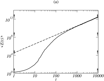
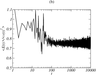
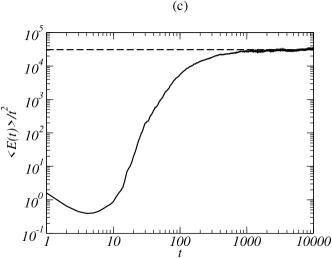
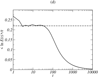
Figure 5: Duffing oscillator: Eq. (8) is integrated numerically for $\omega=1$, $\lambda=10^{-6}$ and ${\mathcal{D}}=1$ with a timestep $\delta t=10^{-4}$. Ensemble averages are computed over $2\,10^{3}$ realizations. Fig. (a): $\langle E(t)\rangle$ vs. $t$; the dashed line corresponds to the expected power law $\langle E(t)\rangle\simeq D_{E}(\lambda)\;t^{2}$. Fig. (b): the numerical value of the equipartition ratio $\langle E(t)\rangle/\langle v(t)^{2}\rangle$ changes from a value close to $1$ to $3/4$. Fig. (c): the numerical estimate of the generalized diffusion constant $D_{E}(\lambda)=\lim_{t\rightarrow\infty}\langle E(t)\rangle/t^{2}$ is $3.0(4)\,10^{4}$; the dashed line corresponds to the expected diffusion constant $D_{E}(\lambda)=3.13\,10^{4}$. Fig. (d): $\langle\ln E(t)\rangle/t$ vs. time $t$; the dashed line corresponds to the Lyapounov exponent $\Lambda=0.22$ expected in the linear regime.

When $\omega$ is non zero, Eqs. (11) and (12) become:

$$x = \left(\frac{4E^{2}}{4E+\omega^{4}}\right)^{1/4}\frac{{\rm sn}\left((4E+\omega^{4})^{\frac{1}{4}}t;k\right)}{{\rm dn}\left((4E+\omega^{4})^{\frac{1}{4}}t;k\right)},$$ (48)

$$\dot{x} = (2E)^{1/2}\frac{{\rm cn}\left((4E+\omega^{4})^{\frac{1}{4}}t;k\right)}{{\rm dn}^{2}\left((4E+\omega^{4})^{\frac{1}{4}}t;k\right)},$$ (49)

where the elliptic modulus $k$ varies with the energy and is given by

$$k^{2}=\frac{\sqrt{4E+\omega^{4}}-\omega^{2}}{2\sqrt{4E+\omega^{4}}}.$$ (50)

We notice that $k$ tends to the limiting value $1/\sqrt{2}$ when the energy goes to infinity. Defining the angle variable as:

$$\phi={\rm sd}^{-1}\left(\frac{(4E+\omega^{4})^{\frac{1}{4}}}{\sqrt{2E}}\,x;\,k\right),$$ (51)

we rewrite the dynamical equation in energy-angle coordinates. However, while deriving the dynamical equation for $\phi$ we must remember that the elliptic modulus $k$ depends on the energy $E$ and is, therefore, a function of time. After reintroducing the multiplicative noise term, the stochastic Duffing oscillator in the energy-angle variables becomes:

$$\dot{E} = \frac{2E}{(4E+\omega^{4})^{\frac{1}{4}}}\,\frac{{\rm sn}(\phi;k){\rm cn}(\phi;k)}{{\rm dn}^{3}(\phi;k)}\,\xi(t)\,\,;$$ (52)

$$\dot{\phi} = (4E+\omega^{4})^{\frac{1}{4}}-\xi(t)\frac{(2E+\omega^{4}){\rm sd}^{2}(\phi;k)}{(4E+\omega^{4})^{\frac{5}{4}}}-\omega^{2}\xi(t)\left(\frac{\,E\,{\rm sd}^{4}(\phi;k)}{(4E+\omega^{4})^{\frac{7}{4}}}\,-\frac{E\,{\rm sn}(\phi;k){\rm cn}(\phi;k)\int_{0}^{\phi}{\rm sd}^{2}(\theta;k)d\theta}{(4E+\omega^{4})^{\frac{7}{4}}{\rm dn}^{3}(\phi;k)}\,\right)\,.$$ (53)

As compared to Eq. (20), two supplementary terms appear in Eq. (53). These terms are related to ${dk}/{dt}$ and are proportional to $\omega^{2}$.

Although the dynamical equations are more complicated than those of the purely cubic case, the analysis can be performed as above. We shall however simplify our discussion here by taking $k$ equal to its asymptotic value $1/\sqrt{2}$. This approximation is justified as soon as the energy is large. We also replace the noise $\xi(t)$ by the effective noise $\Xi(t)$ defined in Eq. (35). This second approximation is only qualitatively correct since it amounts to neglecting a deterministic force in the effective Langevin dynamics for $E$. We thus obtain:

$$\dot{E}\simeq\frac{2E}{(4E+\omega^{4})^{\frac{1}{4}}}\,\Xi(t)\,.$$ (54)

We deduce from Eq. (54) that as long as $E\ll\omega^{4}$, the energy behaves as the exponential of a Brownian motion and, therefore, increases exponentially with time. However, when $E>\omega^{4}$, the nonlinear term becomes important, Eq. (52) reduces to Eq. (18), and the energy grows as the square of time.

We expect that the crossover from exponential to algebraic growth will appear when $E\sim\omega^{4}$, or $x\sim\omega$. Using unscaled variables, the balance between linear and non-linear terms in Eq. (8) is obtained when $x=x_{c}\sim\omega/\sqrt{\lambda}$. Fig. 5 demonstrates that the two regimes are observed numerically when the nonlinear coefficient $\lambda$ is very small compared to $\omega^{2}$: we use the numerical values $\omega=1$ and $\lambda=10^{-6}$. We notice that in the short-time linear regime, the usual equipartition relation for a quadratic potential is verified ($\langle E\rangle\simeq\langle\dot{x}^{2}\rangle$), while the exponential growth of the energy is characterized by the Lyapunov exponent $\Lambda$ defined in Eq. (7). In the long-time regime, the equipartition ratio reaches its nonlinear value $3/4$, while the energy growth becomes algebraic, with a generalized diffusion constant $D_{E}(\lambda)$ in good agreement with Eq. (40), up to the expected scaling factor: $D_{E}(\lambda)=D_{E}/\lambda$.

IV The general nonlinear oscillator with parametric noise

We now consider the case of a particle trapped in a confining potential ${\mathcal{U}}(x)$ and subject to an external noise. This mechanical system generalizes the Duffing oscillator studied in the previous section and its dynamics is given by

$$\frac{\textrm{d}^{2}}{\textrm{d}t^{2}}x(t)+\xi(t)\,x(t)=-\frac{\partial{\mathcal{U}}(x)}{\partial x}\,,$$ (55)

where $\xi(t)$ is the Gaussian white noise of Eq. (2). For the potential to be confining, we must have ${\mathcal{U}}\rightarrow+\infty$ when $|x|\rightarrow\infty$. We restrict our analysis to the case where ${\mathcal{U}}$ is a polynomial; in order to respect the $x\to-x$ symmetry ${\mathcal{U}}$ is even in $x$. Hence, when $|x|\rightarrow\infty$,

$${\mathcal{U}}\sim\frac{x^{2n}}{2n}\,\,\hbox{ with }\,\,n\geq 2\,,$$ (56)

the coefficient of $x^{2n}$ is chosen to be $1/2n$ by a suitable rescaling. As before, we expect the amplitude of the oscillator to grow without bounds at large times. Keeping only the relevant terms in Eq. (55) leads to

$$\frac{\textrm{d}^{2}}{\textrm{d}t^{2}}x(t)+\xi(t)\,x(t)+x(t)^{2n-1}=0\,.$$ (57)

The deterministic version of Eq. (57), $\ddot{x}+x^{2n-1}=0$, is integrable because of energy conservation. For a given value of $E$ the deterministic solution is

$$x = E^{1/{2n}}\,{\mathcal{S}}_{n}\left((2nE)^{\frac{n-1}{2n}}t\right),$$ (58)

$$\dot{x} = (2n)^{\frac{n-1}{2n}}E^{1/2}\,{\mathcal{S}}_{n}^{\prime}\left((2nE)^{\frac{n-1}{2n}}t\right)\,,$$ (59)

where the energy reads

$$E=\frac{1}{2}\dot{x}^{2}+\frac{1}{2n}x^{2n}\,.$$ (60)

The function ${\mathcal{S}}_{n}$ is defined as the inverse function of an hyperelliptic integral as follows

$${\mathcal{S}}_{n}(X)=Y\,\leftrightarrow X=\sqrt{n}\int_{0}^{\frac{Y}{(2n)^{1/2n}}}\frac{{\textrm{d}}u}{\sqrt{1-u^{2n}}}=\frac{\sqrt{n}}{(2n)^{1/2n}}\int_{0}^{Y}\frac{{\textrm{d}}u}{\sqrt{1-\frac{u^{2n}}{2n}}}\,.$$ (61)

From this definition, we find a relation between ${\mathcal{S}}_{n}$ and its derivative ${\mathcal{S}}_{n}^{\prime}$

$${\mathcal{S}}_{n}^{\prime}(X)=\frac{(2n)^{\frac{1}{2n}}}{\sqrt{n}}\left(1-\frac{({\mathcal{S}}_{n}(X))^{2n}}{2n}\right)^{\frac{1}{2}}.$$ (62)

The action-angle variables for the deterministic system are given by

$$I = 4\int_{0}^{(2nE)^{\frac{1}{2n}}}\sqrt{2E-\frac{x^{2n}}{n}}{\textrm{d}}x=4\,(2^{n+1}n)^{\frac{1}{2n}}\,E^{\frac{n+1}{2n}}\int_{0}^{1}\sqrt{1-u^{2n}}{\textrm{d}}u\propto E^{\frac{n+1}{2n}}\,,$$ (63)

$$\phi = {\mathcal{S}}_{n}^{-1}\left(\frac{x}{E^{\frac{1}{2n}}}\right)=\sqrt{n}\,\int_{0}^{\frac{x}{(2nE)^{{1}/{2n}}}}\frac{{\textrm{d}}u}{\sqrt{1-u^{2n}}}\,.$$ (64)

The angle variable $\phi$ is well defined modulo the period $4K_{n}$ of the function ${\mathcal{S}}_{n}$ where

$$K_{n}=\sqrt{n}\int_{0}^{1}\frac{{\textrm{d}}u}{\sqrt{1-u^{2n}}}\,.$$ (65)

When the noise term is taken into account, the energy is not conserved and the stochastic evolution of the variables $E$ and $\phi$ is given by

$$\dot{E} = x\dot{x}\xi(t)=(2n)^{\frac{n-1}{2n}}\,E^{\frac{n+1}{2n}}\,{\mathcal{S}}_{n}(\phi){\mathcal{S}}_{n}^{\prime}(\phi)\,\xi(t)\,,$$ (66)

$$\dot{\phi} = (2nE)^{\frac{n-1}{2n}}-\frac{1}{(2n)^{\frac{1}{n}}}\,\frac{{\mathcal{S}}_{n}(\phi)^{2}}{(2nE)^{\frac{n-1}{2n}}}\,\xi(t)\,.$$ (67)

Introducing the auxiliary variable $\Omega$,

$$\Omega=(2n)^{\frac{n+1}{2n}}\,E^{\frac{n-1}{2n}}\,,$$ (68)

the Eqs. (66) and (67) can be written in the simpler form:

$$\dot{\Omega} = (n-1)\,{\mathcal{S}}_{n}(\phi){\mathcal{S}}_{n}^{\prime}(\phi)\,\xi(t)\,,$$ (69)

$$\dot{\phi} = \frac{\Omega}{(2n)^{\frac{1}{n}}}-\frac{{\mathcal{S}}_{n}(\phi)^{2}}{\Omega}\,\xi(t)\,.$$ (70)

As in the case of the Duffing oscillator, we observe that $\phi$ is a fast variable and therefore we shall average out its rapid variations. Starting from (59), we write

$$\langle\dot{x}^{2}\rangle=(2n)^{\frac{n-1}{n}}\,\overline{{\mathcal{S}}_{n}^{\prime}(\phi)^{2}}\,\langle E\rangle=2\,\frac{\int_{0}^{1}\textrm{d}u\,\sqrt{1-u^{2n}}}{\int_{0}^{1}\frac{\textrm{d}u}{\sqrt{1-u^{2n}}}}\,\langle E\rangle\,,$$ (71)

the last equality is derived by writing $u={\mathcal{S}}_{n}(\phi)$, and using Eqs. (62) and (65). Moreover, the following identity is true (as can be shown by integrating $\int_{0}^{1}1.\sqrt{1-u^{2n}}\,\textrm{d}u$ by parts):

$$\int_{0}^{1}\textrm{d}u\,\sqrt{1-u^{2n}}=n\int_{0}^{1}\textrm{d}u\,\frac{u^{2n}}{\sqrt{1-u^{2n}}}=-n\int_{0}^{1}\textrm{d}u\,\sqrt{1-u^{2n}}+n\int_{0}^{1}\frac{\textrm{d}u}{\sqrt{1-u^{2n}}}\,.$$ (72)

Substituting this identity in Eq. (71) leads to

$$\langle E\rangle=\frac{n+1}{2n}\,\langle\dot{x}^{2}\rangle.$$ (73)

From the definition (60) of the energy, we derive another statistical equality:

$$\langle\dot{x}^{2}\rangle=\langle x^{2n}\rangle\,.$$ (74)

We emphasize again that these generalized equipartition relations are valid for any type of noise, colored or white, additive or multiplicative. The only hypothesis is that the probability distribution function $P_{t}(\Omega,\phi)$ becomes uniform in $\phi$ over the interval $[0,4K_{n}]$ when $t\rightarrow\infty$. We observe from the numerical simulations presented in Fig. 6.c that this condition is very well satisfied.

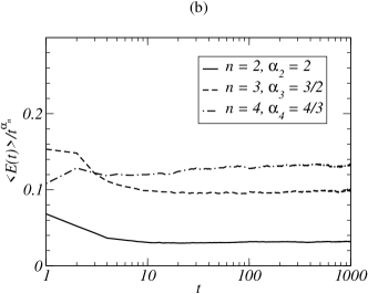
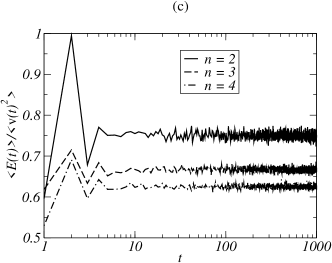
Figure 6: General nonlinear oscillator: Eq. (57) is integrated numerically for ${\mathcal{D}}=1$, with a timestep $\delta t$, and averaged over $10^{4}$ realizations for $n=2$ ($2n-1=3$), $\delta t=5\,10^{-4}$; $n=3$ ($2n-1=5$), $\delta t=5\,10^{-4}$; $n=4$ ($2n-1=7$), $\delta t=10^{-4}$. Fig. (a): average energy $\langle E(t)\rangle$ vs. time $t$. Fig. (b): the limit $\lim_{t\rightarrow\infty}\langle E(t)\rangle/t^{\alpha_{n}}$, $\alpha_{n}=\frac{n}{n-1}$, yields the following estimates of the diffusion constants $D_{E}^{(n)}$: $D_{E}^{(2)}=0.031(1)$, $D_{E}^{(3)}=0.097(3)$, $D_{E}^{(4)}=0.130(5)$, in excellent agreement with the predictions of Eqs. (86) and (87). Fig. (c): the measured equipartition ratio $\langle E(t)\rangle/\langle v(t)^{2}\rangle$ is close to the theoretical value $\frac{n+1}{2n}$ given in Eq. (73): $3/4$ for $n=2$; $2/3$ for $n=3$; $5/8$ for $n=4$. Data for $n=2$ is the same as that of Figs. 2 and 3.

The averaging process with respect to the fast variable generates an effective Langevin dynamics for the slow variable $\Omega(t)$. Starting from the Fokker-Planck equation for the total P.D.F., $P_{t}(\Omega,\phi),$ and averaging over $\phi$ leads to the following evolution equation for the averaged probability distribution ${\tilde{P}}_{t}(\Omega)$

$$\partial_{t}{\tilde{P}}=\frac{{\mathcal{M}}_{n}{\mathcal{D}}}{2}\left(\partial_{\Omega}^{2}{\tilde{P}}-\frac{2}{n-1}\,\partial_{\Omega}\frac{{\tilde{P}}}{\Omega}\right)\,,$$ (75)

where ${\mathcal{M}}_{n}$ is given by

$${\mathcal{M}}_{n}=\frac{(n-1)^{2}}{n}\,(2n)^{\frac{2}{n}}\,\frac{\int_{0}^{1}{\textrm{d}}u\,u^{2}\sqrt{1-u^{2n}}}{\int_{0}^{1}\frac{{\textrm{d}}u}{\sqrt{1-u^{2n}}}}=\frac{(n-1)^{2}}{n+1}\,(2n)^{\frac{2}{n}}\,\frac{\Gamma(\frac{3}{2n})}{\Gamma(\frac{1}{2n})}\,\frac{\Gamma(\frac{3n+1}{2n})}{\Gamma(\frac{3n+3}{2n})}\,,$$ (76)

$\Gamma(.)$ being the Euler Gamma function. The effective Langevin dynamics for the variable $\Omega$ is thus

$$\dot{\Omega}=\frac{{\mathcal{M}}_{n}\,{\mathcal{D}}}{n-1}\,\frac{1}{\Omega}+\Xi_{n}(t)\,,$$ (77)

where the effective Gaussian white noise $\Xi_{n}(t)$ satisfies the relation

$$\langle\Xi_{n}(t)\,\Xi_{n}(t^{\prime})\rangle={\mathcal{M}}_{n}{\mathcal{D}}\,\delta(t-t^{\prime})\,.$$ (78)

The averaged distribution fonction ${\tilde{P}}_{t}(\Omega)$ can be calculated because Eq. (75) is exactly solvable due to its invariance under rescalings $t\rightarrow\lambda^{2}t$ , $\Omega\rightarrow\lambda\Omega\,,$ $\lambda$ being an arbitrary real number. The P.D.F. of $\Omega$ is found to be

$${\tilde{P}}_{t}(\Omega)=\frac{1}{\Gamma\left(\frac{n+1}{2(n-1)}\right)}\,\frac{\Omega^{\frac{2}{n-1}}}{\left(2{\mathcal{M}}_{n}{\mathcal{D}}t\right)^{\frac{n+1}{2(n-1)}}}\,\exp\left\{-\frac{\Omega^{2}}{2{\mathcal{M}}_{n}{\mathcal{D}}t}\right\}\,,$$ (79)

from which we obtain the P.D.F. of the energy:

$${\tilde{P}}_{t}(E)=\frac{1}{\Gamma\left(\frac{n+1}{2(n-1)}\right)}\,\frac{n-1}{nE}\,\left(\frac{(2n)^{\frac{n+1}{n}}\;E^{\frac{n-1}{n}}}{2{\cal M}_{n}{\cal D}t}\right)^{\frac{n+1}{2(n-1)}}\exp\left\{-\frac{(2n)^{\frac{n+1}{n}}\;E^{\frac{n-1}{n}}}{2{\cal M}_{n}{\cal D}t}\right\}\,.$$ (80)

The long-time behavior of the amplitude, velocity and energy of the general nonlinear oscillator can now be derived. Using the equipartition identity (73) and Eq. (80), we obtain

$$\langle E\rangle = \frac{1}{(2n)^{\frac{n+1}{n-1}}}\frac{\Gamma\left(\frac{3n+1}{2n-2}\right)}{\Gamma\left(\frac{n+1}{2n-2}\right)}\left(2{\mathcal{D}}{\mathcal{M}}_{n}t\right)^{\frac{n}{n-1}}\propto t^{\frac{n}{n-1}}\,,$$ (81)

$$\langle\dot{x}^{2}\rangle = \frac{2n}{n+1}\langle E\rangle\propto t^{\frac{n}{n-1}}\,.$$ (82)

Using Eq (76), we find that

$$\overline{{\mathcal{S}}_{n}^{2}(\phi)}=\frac{1}{K_{n}}\int_{0}^{K_{n}}{\mathcal{S}}_{n}^{2}(\phi)\,{\textrm{d}}\phi=(2n)^{\frac{1}{n}}\frac{\int_{0}^{1}\frac{u^{2}{\textrm{d}}u}{\sqrt{1-u^{2n}}}}{\int_{0}^{1}\frac{{\textrm{d}}u}{\sqrt{1-u^{2n}}}}=\frac{n+3}{(2n)^{\frac{1}{n}}(n-1)^{2}}{\mathcal{M}}_{n}\,,$$ (83)

where we made the change of variables $u={\mathcal{S}}_{n}(\phi),$ and used the following identity (obtained by integrating by parts):

$$\int_{0}^{1}u^{2}\sqrt{1-u^{2n}}\,{\textrm{d}}u=\frac{n}{n+3}\,\int_{0}^{1}\frac{u^{2}{\textrm{d}}u}{\sqrt{1-u^{2n}}}\,.$$ (84)

Finally, we deduce from Eqs. (58), (80) and (83)

$$\langle x^{2}\rangle=\overline{{\mathcal{S}}_{n}^{2}(\phi)}\,\langle E^{1/n}\rangle=\frac{2}{n-1}\,\frac{{\cal M}_{n}}{(2n)^{\frac{1}{n}}}\,\frac{\Gamma\left(\frac{3n+1}{2n-2}\right)}{\Gamma\left(\frac{n+1}{2n-2}\right)}\,\left(\frac{2{\mathcal{M}}_{n}{\mathcal{D}}t}{(2n)^{\frac{n+1}{n}}}\right)^{\frac{1}{n-1}}\propto t^{\frac{1}{n-1}}\,.$$ (85)

The analytical results for the nonlinear oscillators with quintic $x^{5}$ ($n=3$) and heptic nonlinearity $x^{7}$ ($n=4$) are as follows:

$$\hbox{For $n=3$}, \,\,\langle E\rangle=0.097\,t^{3/2}\,\,\,,\,\,\,\langle\dot{x}^{2}\rangle=0.145\,t^{3/2}\,\,\,,\,\,\,\langle x^{2}\rangle=0.290\,t^{1/2}\,\,.$$ (86)

$$\hbox{For $n=4$}, \,\,\langle E\rangle=0.130\,t^{4/3}\,\,\,,\,\,\,\langle\dot{x}^{2}\rangle=0.208\,t^{4/3}\,\,\,,\,\,\,\langle x^{2}\rangle=0.347\,t^{1/3}\,\,.$$ (87)

The formulas (81), (82) and (85) were verified numerically. The scaling exponents and the prefactors given in Eqs. (86) and (87) are in excellent agreement with the numerical values, as shown in Fig. 6.

In conclusion, we have derived the following scaling relations:

$$E \sim t^{\frac{n}{n-1}},$$

$$x \sim t^{\frac{1}{2(n-1)}},$$

$$\dot{x} \sim t^{\frac{n}{2(n-1)}}.$$ (88)

In particular, it should be remarked that $x$ undergoes an anomalous diffusion with time with exponent $1/{(2n-2)}$. If we make $n\to 1$ formally, this exponent diverges to infinity: this is consistent with the exponential growth of the linear oscillator (see Sec. II).

We end this section by considering the case of a general confining potential energy ${\mathcal{U}}$ neither necessarily polynomial in $x$ nor even in $x$. The only requirement is that ${\mathcal{U}}\rightarrow+\infty$ when $|x|\rightarrow\infty$. We discuss the qualitative behavior of $E$, $\dot{x}$ and $x$ at large times from elementary scaling considerations. Suppose first that ${\mathcal{U}}\sim|x|^{r}$ for large values of $|x|$, $r$ being an arbitrary real number.

• If $r>2$, then balance between kinetic and potential energies leads to $E\sim\dot{x}^{2}\sim x^{r}$; thus the time evolution of the energy is given by $\dot{E}\sim x\dot{x}\xi\sim E^{\frac{1}{r}-\frac{1}{2}}\xi$. From the scaling relations $\dot{E}\sim E/t$ and $\xi\sim t^{-1/2}$, we conclude that

  $$E\sim t^{\frac{r}{r-2}},\,\,\,\,x\sim t^{\frac{1}{r-2}},\,\,\,\,\dot{x}\sim t^{\frac{r}{2(r-2)}}\,\,.$$

  This qualitative argument can be made rigorous by generalizing the results obtained above to non-integer values of $r$.

• If $r\leq 2$, then the potential ${\mathcal{U}}$ is negligible with respect to the multiplicative noise term and we are back to the case of the degenerate linear oscillator. Therefore $E$, $\dot{x}$ and $x$ grow exponentially with time.

If the potential grows exponentially, i.e. ${\mathcal{U}}\sim{\rm e}^{x^{\beta}}$, $\beta$ being a positive real number, then similar considerations lead to $E\sim t$ and $\dot{x}\sim t^{1/2}$ (leaving aside logarithmic corrections). We then conjecture that the amplitude $x$ diffuses in a logarithmically slow manner: $x\sim(\ln t)^{1/\beta}$.

V Colored Gaussian noise

We now consider the case where the Gaussian noise has a non-zero correlation time, and discuss how the previously found scalings are modified. The system we want to study satisfies the dynamical equation:

$$\frac{\textrm{d}^{2}}{\textrm{d}t^{2}}x(t)+x(t)\,\eta(t)+x(t)^{2n-1}=0,$$ (89)

where $\eta$ is a colored Gaussian noise of zero mean-value. The statistical properties of $\eta$ are determined by

$$\langle\eta(t)\rangle = 0\,,$$

$$\langle\eta(t)\eta(t^{\prime})\rangle = \frac{\mathcal{D}}{2\,\tau}\,{\rm e}^{-|t-t^{\prime}|/\tau}\,,$$ (90)

where $\tau$ is the correlation time of the noise. The noise $\eta$ can be obtained from white noise by solving the Ornstein-Uhlenbeck equation:

$$\frac{{\textrm{d}}\eta(t)}{{\textrm{d}}t}=-\frac{1}{\tau}\eta(t)+\frac{1}{\tau}\xi(t),$$ (91)

where $\xi(t)$ is the Gaussian white noise defined in Eq. (2), and $t,t^{\prime}\gg\tau$.

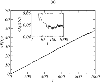
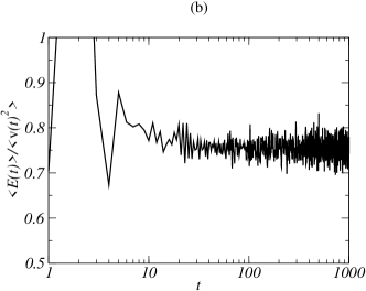
Figure 7: Cubic oscillator with colored noise. Eqs. (89,91) are integrated numerically for $n=2$, $2n-1=3$, ${\mathcal{D}}=1$, $\tau=1$, with a timestep $\delta t=10^{-5}$. Ensemble averages are computed over $10^{3}$ realizations. Fig. (a): the average energy $\langle E(t)\rangle$ grows linearly with time. The inset gives an estimate of the diffusion constant $D_{E}\simeq 0.047(3)$. Fig. (b): the time-asymptotic value of the equipartition ratio $\langle E(t)\rangle/\langle v(t)^{2}\rangle$ is equal to $3/4$.

Introducing action-angle variables as in Sec. IV, we obtain the same set of coupled Langevin equations, Eqs. (69,70), where $\xi(t)$ is replaced by the colored noise $\eta(t)$. As emphasized previously, the generalized equipartition relations are independent of the nature of the noise: Eqs. (73) and (74) remain valid when the noise is correlated in time. This is confirmed by numerical simulations (see Fig. 7.b for $n=2$).

The scalings found in sections III and IV are deduced by averaging the Fokker-Planck equation. Here, we must write the evolution equation for the joint P.D.F. of $x$, $v=\dot{x}$ and $\eta$, $P_{t}(x,v,\eta)$:

$$\frac{\partial P}{\partial t}=-v\frac{\partial P}{\partial x}+(x^{2n-1}-x\eta)\frac{\partial P}{\partial v}+\frac{1}{\tau}\frac{\partial\eta P}{\partial\eta}+\frac{{\mathcal{D}}}{2\tau^{2}}\frac{\partial^{2}P}{\partial\eta^{2}}\,.$$ (92)

We perform a scaling analysis of this equation in the spirit of yp . Balancing the diffusion term with the time derivative leads to $\eta\sim t^{1/2}$. Then we compare the terms of probability current $\frac{vP}{x}$ and $\frac{(x^{2n-1}-x\eta)P}{v}.$ A consistent balance between these terms is possible only if $v^{2}\sim x^{2n}$ and $x^{2n-2}\sim\eta$. We thus find the following scaling relations

$$E \sim t^{\frac{n}{2(n-1)}},$$

$$x \sim t^{\frac{1}{4(n-1)}},$$

$$\dot{x} \sim t^{\frac{n}{4(n-1)}}.$$ (93)

Thus, we predict that the scaling exponents for colored noise are half the exponents calculated for white noise (88). Numerical simulations indeed confirm that the average energy of a cubic oscillator ($n=2$) with colored multiplicative noise grows linearly with time (see Fig. 7.a).

The period $T$ of a deterministic oscillator (without noise) decreases as the energy increases: $T\sim E^{-\frac{n-1}{2n}}$ from Eq. (67). When the equations are written in the energy-angle coordinates, two time scales $T$ and $\tau$ appear. In the regime where $\tau\ll T$, the correlation time of the noise is much smaller than the typical variation time of the angle. Hence the noise can be considered to be white, the averaging procedure can be applied as in Section IV and the scalings found in (88) are correct. When $T\sim\tau$ the noise becomes correlated over a period of the free system and can not be treated as white anymore. Now, $T\sim\tau$ corresponds to $E\sim\tau^{-\frac{2n}{n-1}}$ which leads to crossover time $t_{c}$ of the order $t_{c}^{\frac{n}{n-1}}\sim\tau^{-\frac{2n}{n-1}}$ i.e. $t_{c}\sim\tau^{-2}$. For times larger than $t_{c}$, the scalings (93) are observed.

VI Conclusion

A particle trapped in a confining potential with white multiplicative noise undergoes anomalous diffusion: if the confining potential grows as $x^{2n}$ at infinity, the particle diffuses as $D_{x}t^{\beta_{n}}$. We have calculated the anomalous diffusion exponent $\beta_{n}=1/(2n-2)$, and the coefficient $D_{x}$. We have found similar laws for the diffusion of velocity and energy. Thanks to generalized equipartition identities, we have derived universal relations between the exponents and between the prefactors. Our calculations are based on the assumption that in the long-time limit the probability distribution function becomes uniform in the phase variable. By averaging out the phase variations, an effective, projected, dynamics for the action (or energy) can be defined. This technique enabled us to derive the asymptotic distribution law of the energy in the $t\to\infty$ limit, and to calculate its non-Gaussian features (skewness and flatness). Our analytical results agree with the numerical simulations within the numerical error bars. Thus, the averaging procedure produces very accurate results; it would be an interesting and challenging problem to characterize deviations from our results and to calculate subleading corrections.

In the case of colored multiplicative noise, we have deduced the anomalous diffusion exponents from an elementary scaling argument. Our result, supported by numerics, shows that the exponents are halved in presence of time correlations. The efficiency of parametric amplification decreases if the noise is coherent over a period of the system and therefore the particle diffuses at a much slower rate. In this case, however, the averaging technique is harder to apply because the noise itself is averaged out to the leading order. A precise calculation in the case of colored Gaussian noise still remains to be done.

We have considered only Hamiltonian systems, i.e. systems where no friction is present. Nevertheless, if the damping is small, the results we have derived for the undamped oscillator remain valid until the crossover time (identical to the typical decay time of the energy) is reached. The general case of a non-linear oscillator with (linear) friction leads to interesting results and is currently under study phkir .

Appendix A Nonlinear oscillator with external and internal noise

In this Appendix we discuss the behavior of an oscillator submitted to both additive and multiplicative noises. Because we are considering non-dissipative systems, there is no stationary probability distribution; the position, velocity and energy of the system satisfy scaling laws.

We first consider the case where the noise is only additive. The dynamics of a linear oscillator with additive noise is exactly solvable and the solution of the equation:

$$\frac{\textrm{d}^{2}}{\textrm{d}t^{2}}x(t)+\omega^{2}x(t)=\xi(t),$$ (94)

is given by:

$$x(t)=\frac{1}{\omega}\,\int_{0}^{t}\sin\left(\omega(t-s)\right)\,\xi(s)\,{\textrm{d}}s\,.$$ (95)

We conclude from this expression that $x(t)$ grows diffusively with time:

$$\langle x^{2}(t)\rangle=\frac{{\mathcal{D}}}{2\omega^{2}}\left(t-\frac{\sin 2\omega t}{2\omega}\right).$$ (96)

Such a diffusive behavior is entirely different from the exponential growth of a linear oscillator subject to parametric noise.

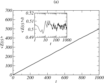
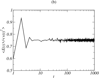
Figure 8: Cubic oscillator with additive noise. Eq. (97) is integrated numerically for ${\mathcal{D}}=1$ with a timestep $\delta t=5\,10^{-4}$. Ensemble averages are computed over $10^{4}$ realizations. Fig. (a): the average energy $\langle E(t)\rangle$ grows linearly with time. The inset gives an estimate of the diffusion constant when noise is additive: $D_{E}\simeq 0.505(5)$. Fig. (b): the time-asymptotic value of the equipartition $\langle E(t)\rangle/\langle v(t)^{2}\rangle$ is equal to $3/4$.

When the nonlinear restoring force is cubic, the linear term can be neglected in the long-time limit and the dynamics is given by

$$\frac{\textrm{d}^{2}}{\textrm{d}t^{2}}x(t)+x(t)^{3}=\xi(t)\,,$$ (97)

where $\xi(t)$ is the Gaussian white noise defined in Eq. (2). This equation can be analyzed as in Sec. III.1. After introducing the energy and angle variables, defined in Eqs. (10) and (19), we obtain

$$\dot{E} = \dot{x}\,\xi(t)=(2E)^{\frac{1}{2}}\,\frac{{\rm cn}(\phi;{1}/{\sqrt{2}})}{{\rm dn}^{2}(\phi;{1}/{\sqrt{2}})}\,\xi(t);$$ (98)

$$\dot{\phi} = (4E)^{\frac{1}{4}}-\frac{{\rm sd}(\phi;{1}/{\sqrt{2}})}{2\sqrt{2}\,E^{1/2}}\,\xi(t).$$ (99)

We can show that the auxiliary variable $\Theta$ defined as

$$\Theta=E^{\frac{1}{2}},$$ (100)

undergoes a normal diffusion process that can be precisely studied after averaging out the fast variable $\phi$. The P.D.F. of the variable $\Theta$, the scaling laws for $E$, $\dot{x}$ and $x$, as well as the generalized diffusion constants can be calculated exactly, as before. We indicate here only the asymptotic power-laws:

$$E \sim t,$$

$$x \sim t^{\frac{1}{4}},$$

$$\dot{x} \sim t^{\frac{1}{2}}.$$ (101)

The scaling exponents for additive noise are different from those for multiplicative noise. For exemple, we observe that a particle submitted to an additive noise in a quartic potential is subdiffusive with an anomalous exponent equal to $1/2$, whereas in the presence of multiplicative noise it behaves diffusively.

In the general case, with a nonlinearity of the type $x^{2n-1}$, with $n\geq 1$, one can prove that the variable $\Theta$, defined in Eq. (100), diffuses as $t^{1/2}$ in the long time limit. Thus the following scalings are satisfied when $t\to\infty$:

$$E \sim t,$$

$$x \sim t^{\frac{1}{2n}},$$

$$\dot{x} \sim t^{\frac{1}{2}}.$$ (102)

All these exponents are smaller than the exponents found for a multiplicative white noise in Eq. (88).

Finally, when both additive and multiplicative noises are present, the oscillator is governed by the equation:

$$\frac{\textrm{d}^{2}}{\textrm{d}t^{2}}x(t)+x(t)\,\xi_{\textrm{mult}}(t)+x(t)^{2n-1}=\xi_{\textrm{add}}(t)\,,$$ (103)

where $\xi_{\textrm{mult}}$ and $\xi_{\textrm{add}}$ are independent white noises of amplitude ${\mathcal{D}}_{\textrm{mult}}$ and ${\mathcal{D}}_{\textrm{add}},$ respectively. If we study the energy variation due to noise, $\dot{E}\sim x\dot{x}\xi_{\textrm{mult}}+\dot{x}\xi_{\textrm{add}}\simeq E^{\frac{n+1}{2n}}\xi_{\textrm{mult}}+E^{1/2}\xi_{\textrm{add}}$, we observe that the first term has a dominant effect. From this simple argument, we conclude that the multiplicative noise is expected to dominate over the additive noise and therefore, asymptotically, the scaling laws will be those derived for the multiplicative noise alone. However, a crossover between the two scalings (88) and (102) should be observed by choosing ${\mathcal{D}}_{mult}\ll{\mathcal{D}}_{add}$. Comparing Eqs. (88) and (102), we find that the effect of the multiplicative noise starts to dominate after a crossover time of the order of $({\mathcal{D}}_{mult}\,t_{c})^{\frac{1}{2n-2}}\sim({\mathcal{D}}_{add}\,t_{c})^{\frac{1}{2n}}$ i.e., $t_{c}\sim{\mathcal{D}}_{add}^{n-1}/{\mathcal{D}}_{mult}^{n}$.

Appendix B Numerical Algorithm

The algorithm used to integrate numerically the stochastic ordinary differential equations studied in this article is the one-step collocation method advocated in mannella . In this Appendix, we recall the general principles underlying this method, and give the algorithms we used to integrate Eqs. (57) and (89)-(91), for white and correlated noise respectively. All stochastic equations are understood according to Stratonovich rules.

Let $\{x_{i}\}_{i=1,\ldots,N}$ be $N$ real variables of time $t$, and $\xi(t)$ a stochastic process assumed to be Gaussian and white. We wish to solve systems of $N$ coupled Langevin equations of the form

$$\dot{x}_{i}=f_{i}(\{x_{j}(t)\})+g_{i}(\{x_{j}(t)\})\;\xi(t),$$ (104)

where $f_{i}$ and $g_{i}$ are $N$ (smooth) functions of the $x_{i}$’s. Let $\delta t$ be the integration timestep. Upon integrating formally Eq. (104) between $0$ and $\delta t$, we obtain the following set of coupled equations implicit in $\{x_{i}(t)\}$

$$x_{i}(\delta t)-x_{i}(0)=\int_{0}^{\delta t}f_{i}(\{x_{j}(s)\})\,\mathrm{d}s+\int_{0}^{\delta t}g_{i}(\{x_{j}(s)\})\;\xi(s)\,\mathrm{d}s.$$ (105)

For $\delta t$ small enough, the functions $f_{i}$ and $g_{i}$ may be Taylor-expanded in the vicinity of $t=0$, e.g.,

$$f_{i}(\{x_{j}(s)\})=f_{i}(\{x_{j}(0)\})+\partial_{k}f_{i}(\{x_{j}(0)\})\,\delta x_{k}(s)+\frac{1}{2}\,\left(\partial_{k}\partial_{l}f_{i}(\{x_{j}(0)\})\right)\,\delta x_{k}(s)\,\delta x_{l}(s)+\ldots\,,$$ (106)

where $\delta x_{k}(s)=x_{k}(s)-x_{k}(0)$. Replacing the functions $f_{i}$ and $g_{i}$ in Eq. (105) by the expansion (106), we obtain a new set of coupled integral equations implicit in $\{\delta x_{i}\}$. Upon solving these equations up to an arbitrary order in $\delta t$, we obtain $\delta x_{k}(\delta t)$. In practice, we implemented an algorithm exact to $O(\delta t^{2})$.

B.1 White noise

We integrate the following set of first-order differential equations

$$\dot{x} = v,$$ (107)

$$\dot{v} = -\omega^{2}x-\lambda x^{2n-1}+x\,\xi,$$ (108)

where the Gaussian white noise $\xi(t)$ verifies Eq. (2). The exact evolution equations for $\delta x(\delta t)=x(\delta t)-x(0)$ and $\delta v(\delta t)=v(\delta t)-v(0)$ read

$$\delta x(\delta t) = \int_{0}^{\delta t}\mathrm{d}s\,\left(v(0)+\delta v(s)\right),$$ (109)

$$\delta v(\delta t) = \int_{0}^{\delta t}\mathrm{d}s\,\left\{-\omega^{2}\,\left(x(0)+\delta x(s)\right)-\lambda\,\left(x(0)+\delta x(s)\right)^{2n-1}+\left(x(0)+\delta x(s)\right)\,\xi(s)\right\}.$$ (110)

The auxiliary variables $Z_{1}$ and $Z_{2}$, defined by

$$Z_{1}(\delta t) = \int_{0}^{\delta t}\xi(s)\,\mathrm{d}s,$$ (111)

$$Z_{2}(\delta t) = \int_{0}^{\delta t}Z_{1}(s)\,\mathrm{d}s,$$ (112)

are Gaussian random variables, with zero average, and the following correlations: $\langle Z_{1}(\delta t)^{2}\rangle={\mathcal{D}}\,\delta t$, $\langle Z_{2}(\delta t)^{2}\rangle={\mathcal{D}}\,\delta t^{3}/3$, $\langle Z_{1}(\delta t)\,Z_{2}(\delta t)\rangle={\mathcal{D}}\,\delta t^{2}/2$. Up to order $(\delta t)^{2}$, we find

$$x(\delta t) = x(0)+v(0)\,\delta t+Z_{2}(\delta t)+\frac{1}{2}\,\delta t^{2}\,\left(-\omega^{2}\,x(0)-\lambda\,x(0)^{2n-1}\right),$$ (113)

$$v(\delta t) = v(0)+Z_{1}(\delta t)+\delta t\,\left(-\omega^{2}\,x(0)-\lambda\,x(0)^{2n-1}\right)+\frac{1}{2}\,\delta t^{2}\,v(0)\left(-\omega^{2}\,x(0)-(2n-1)\,\lambda\,x(0)^{2n-2}\right).$$ (114)

In practice, we use two independent Gaussian random noises $Z_{1}$ and $Y_{1}$ with zero mean and correlations $\langle Z_{1}(\delta t)^{2}\rangle={\mathcal{D}}\,\delta t$, $\langle Y_{1}(\delta t)^{2}\rangle={\mathcal{D}}\,\delta t$. As shown in Ref. mannella , the variable $Z_{2}$ may be approximated by the expression:

$$Z_{2}(\delta t)=\delta t\,\left(\frac{1}{2}Z_{1}(\delta t)+\frac{1}{2\,\sqrt{3}}\,Y_{1}(\delta t)\right),$$ (115)

when the algorithm is exact up to order $\delta t^{2}$.

B.2 Colored noise

When the noise $\eta(t)$ is correlated, we must solve a set of three coupled equations

$$\dot{x} = v,$$ (116)

$$\dot{v} = -\omega^{2}x-\lambda x^{2n-1}+x\,\eta,$$ (117)

$$\dot{\eta} = -\frac{1}{\tau}\,\eta+\frac{1}{\tau}\,\xi.$$ (118)

The set of exact integral equations becomes

$$\delta x(\delta t) = \int_{0}^{\delta t}\mathrm{d}s\,\left(v(0)+\delta v(s)\right),$$ (119)

$$\delta v(\delta t) = \int_{0}^{\delta t}\mathrm{d}s\,\left\{-\omega^{2}\,\left(x(0)+\delta x(s)\right)-\lambda\,\left(x(0)+\delta x(s)\right)^{2n-1}+\left(x(0)+\delta x(s)\right)\,\left(\eta(0)+\delta\eta(s)\right)\right\},$$ (120)

$$\delta\eta(\delta t) = \int_{0}^{\delta t}\mathrm{d}s\,\left\{-\frac{1}{\tau}\,\left(\eta(0)+\delta\eta(s)\right)+\frac{1}{\tau}\,\xi(t)\right\}.$$ (121)

The algorithm to order $\delta t^{2}$ reads

$$x(\delta t) = x(0)+v(0)\,\delta t+\frac{1}{2}\,v(0)\,\delta t^{2}\,,$$ (122)

$$v(\delta t) = v(0)+\delta t\,\left(-\omega^{2}\,x(0)-\lambda\,x(0)^{2n-1}+x(0)\,\eta(0)\right)+\frac{1}{\tau}\,x(0)\,Z_{2}(\delta t)$$ (123)

$$+\frac{1}{2}\,\delta t^{2}\,\left(v(0)\left(-\omega^{2}\,x(0)-(2n-1)\,\lambda\,x(0)^{2n-2}+\eta(0)\right)-\frac{1}{\tau}\,x(0)\,\eta(0)\right),$$

$$\eta(\delta t) = \eta(0)+\frac{1}{\tau}\,Z_{1}(\delta t)+-\frac{1}{\tau}\,\eta(0)\,\delta t-\frac{1}{\tau^{2}}\,Z_{2}(\delta t)+\frac{1}{2}\,\delta t^{2}\,\frac{\eta(0)}{\tau^{2}}.$$ (124)

Appendix C Some useful Properties of Elliptic Functions

The Jacobian elliptic functions ${\rm sn}(u;k),\,{\rm cn}(u;k),\,$ and ${\rm dn}(u;k)$ are meromorphic functions of the complex variable $u$. They depend on a parameter $k$ called the elliptic modulus abram ; byrd . These functions, like the trigonometric functions, have a real period and, like the hyperbolic functions, have an imaginary period. They are thus doubly periodic in the complex plane and their periods are $(4K,2iK^{\prime})$, $(4K,2K+2iK^{\prime})$ and $(2K,4iK^{\prime})$, respectively, where

$$K(k)=\int_{0}^{1}\frac{{\rm d}t}{\sqrt{(1-t^{2})(1-k^{2}t^{2})}}\,\,\,=\int_{0}^{\frac{1}{k^{\prime}}}\frac{{\rm d}y}{\sqrt{(1-{k^{\prime}}^{2}y^{2})(1+k^{2}y^{2})}}\,\,\,\hbox{ with }\,\,\,t^{2}=\frac{y^{2}}{1+k^{2}y^{2}}\,\,\hbox{ and }\,\,\,{k^{\prime}}^{2}=1-k^{2}\,\,.$$ (125)

The imaginary period is given by $K^{\prime}(k)=K(k^{\prime})=K\left(\sqrt{1-k^{2}}\right)\,.$ The Jacobian elliptic functions satisfy the fundamental relations:

$${\rm sn}^{2}(\phi;k)+{\rm cn}^{2}(\phi;k) = 1\,,$$

$$k^{2}{\rm sn}^{2}(\phi;k)+{\rm dn}^{2}(\phi;k) = 1\,,$$ (126)

and their derivatives are

$$\frac{\textrm{d}}{{\textrm{d}}\phi}{\rm sn}(\phi;k) = {\rm cn}(\phi;k)\,{\rm dn}(\phi;k)\,,$$

$$\frac{\textrm{d}}{{\textrm{d}}\phi}{\rm cn}(\phi;k) = -{\rm sn}(\phi;k)\,{\rm dn}(\phi;k)\,,$$

$$\frac{\textrm{d}}{{\textrm{d}}\phi}{\rm dn}(\phi;k) = -k^{2}{\rm sn}(\phi;k)\,{\rm cn}(\phi;k)\,.$$ (127)

If we define the function ${\rm sd}(\phi;k)={\rm sn}(\phi;k)/{\rm dn}(\phi;k)\,,$ the relations (126) and (127) lead to two new formulas

$$\frac{\textrm{d}}{{\textrm{d}}\phi}{\rm sd}(\phi;k)=\frac{{\rm cn}(\phi;k)}{{\rm dn}^{2}(\phi;k)}\,\,\,\hbox{ and }\,\,\,\frac{{\rm cn}^{2}(\phi;k)}{{\rm dn}^{4}(\phi;k)}=(1-{k^{\prime}}^{2}{\rm sd}^{2}(\phi;k))(1+k^{2}{\rm sd}^{2}(\phi;k))\,.$$ (128)

Moreover, from Eqs. (127) and (128), we obtain

$${\rm sn}^{-1}(y;k) = \int_{0}^{y}\frac{{\textrm{d}}t}{\sqrt{(1-t^{2})(1-k^{2}t^{2})}}\,,$$ (129)

$${\rm sd}^{-1}(y;k) = \int_{0}^{y}\frac{{\textrm{d}}u}{\sqrt{(1-{k^{\prime}}^{2}u^{2})(1+k^{2}u^{2})}}\,.$$ (130)

Similar relations can be derived for ${\rm cn}^{-1}$ and ${\rm dn}^{-1}.$ The expressions of inverse elliptic functions in terms of quartic integrals provide a classic way of defining elliptic functions. The change of variables $t=u/\sqrt{1+k^{2}u^{2}}$ in Eq. (129) leads to the identity

$${\rm sd}^{-1}(y;k)={\rm sn}^{-1}\left(\frac{y}{\sqrt{1+k^{2}y^{2}}};k\right)$$ (131)

We deduce from Eq. (129)

$$\frac{\textrm{d}}{{\textrm{d}}k}{\rm sn}^{-1}(y;k)=k\int_{0}^{y}\frac{t^{2}{\textrm{d}}t}{\sqrt{(1-t^{2})(1-k^{2}t^{2})}}=k\int_{0}^{y/\sqrt{1-k^{2}y^{2}}}\frac{u^{2}{\textrm{d}}u}{\sqrt{(1-{k^{\prime}}^{2}u^{2})(1+k^{2}u^{2})}}=k\int_{0}^{\phi_{1}}{\rm sd}^{2}(\phi;k){\textrm{d}}\phi\,,$$ (132)

where the last equality was obtained by setting $u={\rm sd}(\phi;k)$ with $\phi_{1}={\rm sn}^{-1}(y;k)\,.$

We verify from Eqs. (126) and (127) that $x$ and $\dot{x}$ defined in Eqs. (11) and (12) are solutions of the cubic oscillator $\ddot{x}+x^{3}=0.$ Similarly, we verify that $x$ and $\dot{x}$ defined in Eqs. (48) and (49) satisfy the differential equation for the Duffing oscillator, $\ddot{x}+\omega^{2}x+x^{3}=0.$ We now prove the identities used to derive the equipartition relations and the diffusion constants in section III.1. In the case of a purely cubic oscillator, $k=k^{\prime}=1/{\sqrt{2}}\,,$ and we obtain from Eq. (130)

$$\frac{\textrm{d}}{{\textrm{d}}y}{\rm sd}^{-1}(y;\frac{1}{\sqrt{2}})=\frac{1}{\sqrt{1-\frac{y^{2}}{4}}}\,.$$ (133)

From Eq. (128) we deduce

$$\overline{\frac{{\rm cn^{2}}(\phi)}{{\rm dn}^{4}(\phi)}}=\frac{1}{K}\int_{0}^{K}{\rm d}\phi\,\frac{{\rm cn^{2}}(\phi)}{{\rm dn}^{4}(\phi)}=\frac{\int_{0}^{1}\sqrt{1-u^{4}}{\textrm{d}}u}{\int_{0}^{1}\frac{{\textrm{d}}u}{\sqrt{1-u^{4}}}}=\frac{2}{3}\,,$$ (134)

where we have set $u={\rm sd}(\phi)/\sqrt{2}$ to obtain the second equality; the final equality results from Eq. (72). Similarly, we obtain:

$$\overline{\frac{{\rm cn^{4}}(\phi)}{{\rm dn}^{8}(\phi)}}=\frac{1}{K}\int_{0}^{K}{\rm d}\phi\,\frac{{\rm cn^{4}}(\phi)}{{\rm dn}^{8}(\phi)}=\frac{\int_{0}^{1}(1-u^{4})^{\frac{3}{2}}{\textrm{d}}u}{\int_{0}^{1}\frac{{\textrm{d}}u}{\sqrt{1-u^{4}}}}=\frac{4}{7}\,.$$ (135)

The last equality is obtained by the following integration by parts:

$$\int_{0}^{1}1.(1-u^{4})^{\frac{3}{2}}\,{\textrm{d}}u=\int_{0}^{1}6u^{4}(1-u^{4})^{\frac{1}{2}}\,{\textrm{d}}u=\int_{0}^{1}6(1-u^{4})^{\frac{1}{2}}\,{\textrm{d}}u-\int_{0}^{1}6(1-u^{4})^{\frac{3}{2}}\,{\textrm{d}}u\,;$$

thus

$$\int_{0}^{1}(1-u^{4})^{\frac{3}{2}}{\textrm{d}}u=\frac{6}{7}\int_{0}^{1}(1-u^{4})^{\frac{1}{2}}{\textrm{d}}u\,.$$

Now, using Eq. (134), we obtain the numerical value 4/7 in Eq. (135). We also have:

$$\overline{{\rm sd^{2}}(\phi)}=\frac{1}{K}\int_{0}^{K}{\rm d}\phi\,{\rm sd^{2}}(\phi)=2\frac{\int_{0}^{1}\frac{u^{2}{\textrm{d}}u}{\sqrt{1-u^{4}}}}{\int_{0}^{1}\frac{{\textrm{d}}u}{\sqrt{1-u^{4}}}}=\frac{5}{2}{\mathcal{M}},$$ (136)

where ${\mathcal{M}}$ was defined in Eq. (33). The last equality is obtained by using the following identities

$$\int_{0}^{1}\frac{u^{6}{\textrm{d}}u}{\sqrt{1-u^{4}}}=\int_{0}^{1}\frac{u^{3}}{2}\frac{2u^{3}{\textrm{d}}u}{\sqrt{1-u^{4}}}=\frac{3}{2}\int_{0}^{1}u^{2}\sqrt{1-u^{4}}{\textrm{d}}u\,,$$

$$\int_{0}^{1}\frac{u^{2}{\textrm{d}}u}{\sqrt{1-u^{4}}}{\textrm{d}}u=\int_{0}^{1}\left(u^{2}\sqrt{1-u^{4}}+\frac{u^{6}}{\sqrt{1-u^{4}}}\right){\textrm{d}}u=\frac{5}{2}\int_{0}^{1}u^{2}\sqrt{1-u^{4}}{\textrm{d}}u\,.$$

We end this Appendix by explaining how the equations for the phase dynamics are obtained. Eq. (20) is derived from Eqs. (133) and (18):

$$\frac{{\textrm{d}}}{{\textrm{d}}t}\phi=\frac{{\textrm{d}}}{{\textrm{d}}t}{\rm sd}^{-1}\left(\frac{x}{E^{1/4}},\frac{1}{\sqrt{2}}\right)=\frac{\frac{\dot{x}}{E^{1/4}}-\frac{x\dot{E}}{4E^{5/4}}}{\sqrt{1-\frac{x^{4}}{4E}}}=\left(\frac{\dot{x}}{E^{1/4}}-\frac{x^{2}\dot{x}\xi}{4E^{5/4}}\right)\frac{\sqrt{2E}}{\dot{x}}=(4E)^{\frac{1}{4}}-\frac{{\rm sd}^{2}(\phi;{1}/{\sqrt{2}})}{2\sqrt{2}E^{1/4}}\xi(t)\,.$$ (137)

In order to derive the dynamics of the phase of a Duffing oscillator (53), we must differentiate Eq. (51) with respect to time. We must bear in mind that the elliptic modulus $k$ defined in Eq. (50) is now a function of time. Therefore, when differentiating the function ${\rm sd}^{-1}$, we obtain two contributions: $(i)$ the derivative with respect to the argument produces a result similar to the one for the cubic case, $(ii)$ the derivative with respect to the elliptic modulus, calculated using Eqs. (131) and (132), generates the two last terms in Eq. (53).

References

• (1) N.G. van Kampen, Stochastic Processes in Physics and Chemistry, North Holland (1992)
• (2) H. Risken, The Fokker-Planck Equation, Springer-Verlag (1989)
• (3) H. Horsthemke and R. Lefever, Noise Induced Transitions, Springer-Verlag (New-York) (1984)
• (4) P.S. Landa and P.V.E. McClintock, Phys. Rep. 323, 1 (2000)
• (5) C. van den Broeck, J.M.R. Parrondo and R. Toral, Phys. Rev. Lett 73, 3395 (1994)
• (6) C. van den Broeck, J.M.R. Parrondo, R. Toral and R. Kawai, Phys. Rev. E 55, 4084 (1997)
• (7) J.M.R. Parrondo, C. van den Broeck, J. Buceta and F. Javier de la Rubia, Physica A 224, 153 (1996)
• (8) M. San Miguel and R. Toral, Stochastic Effects in Physical Systems in Instabilities and Nonequilibrium Structures VI, E. Tirapegui and W. Zeller Eds. Kluwer Acad. Pub. (1997)
• (9) S. Barbay, G. Giacomelli and F. Marin, Phys. Rev. E 61, 157 (2000)
• (10) R. Bourret, Physica 54, 623 (1971); R. Bourret, U. Frisch and A. Pouquet, Physica 65, 303 (1973)
• (11) M. Lücke and F. Schank, Phys. Rev. Lett 54, 1465 (1985)
• (12) J. Röder, H. Röder and L. Kramer, Phys. Rev. E 55, 7068 (1997)
• (13) W. Genovese and M.A. Muñoz, Phys. Rev. E 60, 69 (1999)
• (14) P. Reimann, Phys. Rep. 361, 57 (2002).
• (15) K. Lindenberg and B. J. West, Physica 128A, 25 (1984)
• (16) R.L. Stratonovich, Topics on the Theory of Random Noise , Gordon and Breach (New-York) Vol 1 (1963) and Vol 2 (1967)
• (17) S. Kabashima, S. Kogure, T. Kawakubo and T. Okada, J. Appl. Phys. 50, 6296 (1979)
• (18) T. Kawakubo, A. Yanagita and S. Kabashima, J. Phys. Soc. Japan 50, 1451 (1981)
• (19) R. Berthet, S. Residori, B. Roman and S. Fauve, Phys. Rev. Lett. 33, 557 (2002)
• (20) J. B. Roberts and M. Vasta, J. Appl. Mechanics 67, 763 (2000)
• (21) P.S. Landa and A.A. Zaikin, Phys. Rev. E 54, 3535 (1996)
• (22) J.P. Bouchaud and A. Georges, Phys. Rep. 195, 127 (1990)
• (23) L. D. Landau and I. Lifshitz, Mechanics , Pergamon Press, Oxford, New York (1969)
• (24) C. van den Broeck, M. Malek Mansour and F. Baras, J. Stat. Phys. 33, 557 (1982)
• (25) F. Drolet and J. Viñals, Phys. Rev. E 57, 5036 (1998)
• (26) V. Seshadri, B. J. West and K. Lindenberg, Physica 107A, 219 (1981)
• (27) D. Hansel and J.F. Luciani, J. Stat. Phys 54, 971 (1989)
• (28) L. Tessieri and F.M. Izrailev, Phys. Rev. E 62, 3090 (2000)
• (29) R. Mannella, Computer experiments in non-linear stochastic physics in Noise in Dynamical systems, Vol. 3: Experiments and simulations, Moss and Mc Clintock Eds. Cambridge University Press, Cambridge (1989)
• (30) C. Degli Esposti Boschi and L. Ferrari, Phys. Rev. E 63, 026218 (2001)
• (31) M. Abramowitz and I. A. Stegun, Handbook of Mathematical Functions, National Bureau of Standards (1966)
• (32) P. F. Byrd and M. D. Friedman, Handbook of elliptic integrals for engineers and physicists , Springer-Verlag (1954)
• (33) A. J. Lichtenberg and M. A. Lieberman, Regular and Chaotic Dynamics, Springer-Verlag (1992)
• (34) Y. Pomeau, J. Phys. I France 3, 365 (1993)
• (35) K. Mallick and P. Marcq, in preparation