Percolation fractal exponents without fractal geometry

Abstract

Classically, percolation critical exponents are linked to the power laws that characterize percolation cluster fractal properties. It is found here that the gradient percolation power laws are conserved even for extreme gradient values for which the frontier of the infinite cluster is no more fractal. In particular the exponent 7/4 which was recently demonstrated to be the exact value for the dimension of the so-called ”hull” or external perimeter of the incipient percolation cluster keeps its value in describing the width and length of gradient percolation frontiers whatever the gradient value. Its origin is then not to be found in the thermodynamic limit. The comparison between numerical results and the exact results that can be obtained analytically for extreme values of the gradient suggests that there exist a unique power law from size 1 to infinity which describes the gradient percolation frontier, this law becoming a scaling law in the large system limit.

Spreading of objects in space with a gradient of probability is most common. From chemical composition gradients to the distribution of plants which depends of their solar exposure, probability gradients exist in many inhomogeneous systems. In fact inhomogeneity is a rule in nature whereas most of the systems that physicists are studying are homogeneous as they are thought to be more simple to understand. In particular phase transitions or critical phenomena are studied in that framework, the simplest being percolation transition[1].

In this work, the opposite situation, a strongly inhomogeneous system is studied. We report the discovery that the validity of some percolation exponents can be extended to situations which are very far from the large homogeneous system limit. This is found in the frame of gradient percolation, a situation first introduced in the study of diffusion front[2, 3]. Surprisingly these exponents, up to now believed to pertain to large systems, are also verified in a limit that could be called the small system limit (S.S.L.) where some of the gradient percolation properties can be computed analytically. This letter presents a report concerning the 2D square lattice. The same results and discussion have been obtained for the triangular lattice and will be published elsewhere, together with the details of the analytical calculations for both lattices.

The gradient percolation (G.P.) situation is depicted in FIG. 1. The figure gives an example of a random distribution of points on a lattice with a linear gradient of concentration in the vertical direction. It is a 2D square lattice of size $L_{g}\times L$, where each point $(x,y)$ is occupied with probability $p(x)=1-x/L_{g}$ ($x$ being the vertical direction in the figure). In gradient percolation there is always an infinite cluster of occupied sites as there is a region where $p$ is larger than the standard percolation (S.P.) threshold $p_{c}$. There is also an infinite cluster of empty sites as there is a region where $p$ is smaller than $p_{c}$. The object of interest is the G.P. front, the external limit (or frontier) of the infinite occupied cluster. It is constituted by the sites which belong to the occupied cluster and are first-nearest neighbours with empty sites belonging to the infinite empty cluster. It is shown in grey in FIG. 1. This front is a random object with an average position $x_{f}$, a statistical width $\sigma_{f}$ and a total length $N_{f}$. In so far that the G.P. front and the S.P. external perimeter (often called hull) have the same geometry their fractal dimension was first conjectured to be exactly equal to 7/4 in [2]. This result was then demonstrated heuristically by Saleur and Duplantier[4] and very recently it was proved mathematically by Smirnov[5].

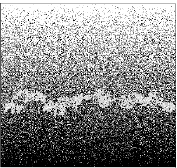
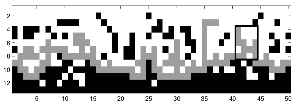
Figure 1: Gradient percolation front. Particles are distributed at random with probability $p(x)=1-x/L_{g}$. The occupied sites are in black and the last line of connected occupied sites is the gradient percolation front shown in light gray. This situation corresponds also to a diffusion situation where the front is called the diffusion front. Top: $L=L_{g}=500$. Bottom: $L=50$ and $L_{g}=12$. The black window has an horizontal width equal to $\sigma_{f}$. It contains approximately $L_{g}$ points.

The early G.P. studies were focussed at finding its relation with standard percolation. Let first recall the definitions. For $0\leq x\leq L_{g}$, $n_{f}(x)$ is the mean number of points of the front lying on the line $x$ per unit horizontal length. It measures the front density at distance $x$. The length $N_{f}$, the position $x_{f}$ and the width $\sigma_{f}$ of the front are then defined in terms of the $n_{f}(x)$ by

$$N_{f}=L\sum_{x=0}^{L_{g}}n_{f}(x),\hskip 5.69046ptx_{f}=\frac{\sum_{x=0}^{L_{g}}xn_{f}(x)}{\sum_{x=0}^{L_{g}}n_{f}(x)},$$

$${\mathrm{and}}\hskip 5.69046pt\sigma_{f}^{2}=\frac{\sum_{x=0}^{L_{g}}(x-x_{f})^{2}n_{f}(x)}{\sum_{x=0}^{L_{g}}n_{f}(x)}.$$

It was found that the mean front was situated at a distance where the density of occupation was very close to $p_{c}$ or $p(x_{f})\simeq p_{c}$. This was verified numerically with such precision that the gradient percolation method is now often used to compute percolation thresholds[6, 7, 8, 9, 10]. It was also found that:

1. The width $\sigma_{f}$ depends on $L_{g}$ through a power law $\sigma_{f}\propto(L_{g})^{\nu/(1+\nu)}$ where $\nu=4/3$ is the correlation length exponent [1] in dimension $d=2$ so that $\sigma_{f}=(L_{g})^{4/7}$. The width $\sigma_{f}$ was also shown to be a percolation correlation length.

2. Secondly it was found that the front was fractal with a dimension $D_{f}$, numerically determined, close to $1.75$. The front length followed a power law $N_{f}\propto(L_{g})^{\alpha_{N}}$ with $\alpha_{N}=(D_{f}-1)\nu/(1+\nu)$.

3. But also, it was numerically observed that the sum of these two exponents was very close to 1. If true this meaned that $\nu/(1+\nu)+(D_{f}-1)\nu/(1+\nu)=1$ or $D_{f}=1+1/\nu$ = 7/4. This is how it was conjectured in [2] that $D_{f}=7/4$.

In that sense the G.P. power laws were thought to be linked to the S.P. exponent $\nu$ and to the fractality of the percolation cluster hull. Up to now, these facts were considered to be strictly valid only in the large system limit.

However, if true, and we know now that 7/4 is the exact value, there follows an intriguing relation, namely $\sigma_{f}^{D_{f}}$ is exactly proportional to $L_{g}^{1}$. This means that the number of surface particles within the correlation length is exactly proportional to $L_{g}$. This is particularly striking for diffusion fronts. Diffusion of particles from a source results in a concentration gradient and an associated G.P. situation. In that frame, the above result means that, if $L_{g}$ particles have diffused on a vertical row, there is on average the same (or a constant fraction of) number of particles on the correlated surface (surface content of a box with a lateral size equal to the statistical width). This fact seems a priori to have nothing to do with scaling, percolation and the thermodynamic limit. From this point of view it is possibly the consequence of a conservation law and if such a conservation exists, it should apply also for extreme gradients corresponding to $L_{g}$ of a few units. In particular it should apply to the very extreme $L_{g}=1$, $2$ and $3$ for which exact values of $x_{f}$, $N_{f}$ and $\sigma_{f}$ can be calculated analytically.

For $L_{g}=2$ or $L_{g}=3$, given a site on a line $x$, one can describe all the configurations such that the point belongs to the front, and compute their probability. For example, for $L_{g}=2$ all the occupied sites on the line $x=1$ belong to the front, and a site on the line $x=0$ will belong to the front if at least one of its three neighbours on the line $x=1$ is empty. Thus we get in this case, $n_{f}(1)=1/2$ and $n_{f}(0)=1-(1/2)^{3}=7/8$. With the same kind of arguments, we can make the computations for $L_{g}=3$ but the geometry of connected sets is more complex as there are more configurations to consider. This however can be done exactly. One obtains: for $L_{g}=1$, $\sigma_{f}=0$;
$\bullet$ for $L_{g}=2$:

$$N_{f}/L=\frac{11}{8},\hskip 5.69046ptx_{f}=\frac{4}{11}\hskip 5.69046pt\mathrm{and}\hskip 5.69046pt\sigma_{f}=\frac{2\sqrt{7}}{11}.$$

$\bullet$ for $L_{g}=3$:

$$N_{f}/L=\frac{9401}{5832},\hskip 5.69046ptx_{f}=\frac{6966}{9401}\hskip 5.69046pt\mathrm{and}\hskip 5.69046pt\sigma_{f}=\frac{9\sqrt{576049}}{9401}.$$

The problem is then to compare the numerical G.P. laws to these exact values. As will be shown, the numerical results verify the above power laws with such precision that the question arises of the existence of a simple mathematical power law extending from $L_{g}=1$ to infinity. To try to answer this question we proceed in 2 steps. First we test these laws on the numerical results obtained for $L_{g}$ between 4 and 50 for the square and triangular lattices by searching the best numerical power laws followed by the width. Considering arbitrary exponents $\alpha$ between $1.6$ and $1.9$, we study $\sigma_{f}^{\alpha}$ as a function of $L_{g}$ between $4$ to $50$. For each $\alpha$ value, there is a best line $\sigma_{f}^{\alpha}=a_{\alpha}(L_{g}+b_{\alpha})$ fitting the numerical $\sigma_{f}^{\alpha}$. The introduction of the term $b_{\alpha}$ is justified by the fact that when a power law is verified for large systems it includes always the possibility that a small (as compared to the system size) term could contribute but in a negligible manner. But here the size itself is small or very small. On the other hand, one should remark that for $L_{g}=1$ the width is strictly 0 so that some negative value of $b_{\alpha}$ should be present. In the next step, the mean error $d(\alpha)$, defined by $d(\alpha)^{2}=(1/47)\sum_{L_{g}=4}^{50}(\sigma_{f}(L_{g})^{\alpha}-a_{\alpha}(L_{g}+b_{\alpha}))^{2}$, is measured numerically as a function of $\alpha$. The results are shown in FIG. 2. There is a clear minimum for $\alpha=1.75$, showing that this exponent gives the best power law fit. Once the best fit with the empirical data is made one has the best values for the parameters $a$ and $b$: $a=0.297$ and $b=-1.09$. Note that $b$ should be strictly equal to $-1$ in order to obtain a null width for the trivial case $L_{g}=1$.

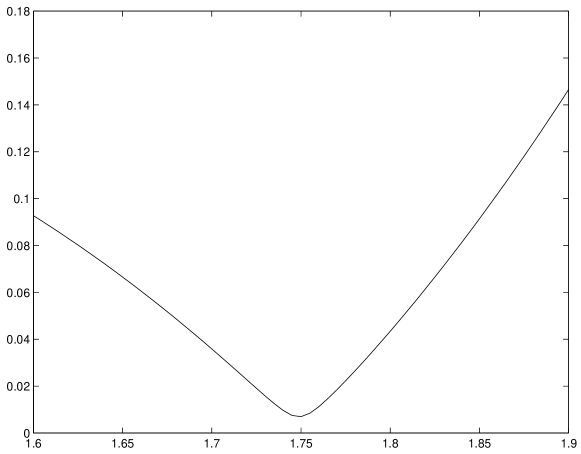
Figure 2: Determination of the best exponent value for the square lattice: $\alpha=1.75$. The same result has been obtained for the triangular lattice.

An other verification of the extreme G.P. power laws can be obtained from the study of the front length or of the quantity $(N_{f}/L)^{7/3}$ as a function of $L_{g}$. In FIG. 3, the diamonds represent the values of $(N_{f}/L)^{7/3}$ and the best linear fit has equation $Y=c(L_{g}+d)$ with $c=0.845$ and $d=0.88$. This shows indeed that the exponents $4/7$ and $3/7$ can be used down to the steepest gradients for which the frontier is no more fractal.

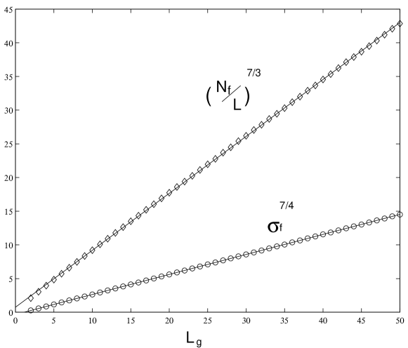
Figure 3: Numerical results for the square lattice. The circles resp. diamonds represent respectively $\sigma_{f}^{7/4}$ and $(N_{f}/L)^{7/3}$.

One can then extrapolate the $\sigma_{f}$ values to the case $L_{g}=1$, $2$ and $3$. The results are given in Table I. One observes that the numerical extrapolations correspond to the exact values with an apparent good precision. However no firm conclusion can be drawn without discussion of the numerical uncertainties. The values shown on FIG. 3 are averaged over $50$ trials on a length $L=10^{5}$. As the fit occurs through a power law it is difficult to give a confidence interval for the coefficients $a$ and $b$ (obtained from a least square linear regression on the values of $\sigma_{f}^{7/4}$).

In order to obtain a better control on the numerical precision of $a$ and $b$ we made extensive computations of the two cases $L_{g}=4$ and $L_{g}=5$ with 100 trials on a length $L=5.10^{5}$. Doing so we obtain the mean values with their standard deviation: $\sigma_{f}(4)^{7/4}=0.8658\pm 0.0009$ and for $\sigma_{f}(5)^{7/4}=1.1610\pm 0.0013$. Thus if we compute the equation of the line $\overline{a}(L_{g}+\overline{b})$ which interpolates the two points $(4,\sigma_{f}(4)^{7/4})$ and $(5,\sigma_{f}(5)^{7/4})$, we obtain $\overline{a}=0.2952\pm 0.0022$ and $\overline{b}=-1.066\pm 0.041$. This last result shows that the value $-1$ is not incompatible with $\overline{b}$ and its statistical error. Given the numerical values for $L_{g}=4$ and $5$, we can also get extrapolated values for $\sigma_{f}$ for $L_{g}$ smaller, together with their confidence interval. The result (see Table I) is that the predicted values are very close to the exact ones. For $(N_{f}/L)^{7/3}$, in the same way we obtain a linear interpolate of the values for $L_{g}=4$ and $5$, with coefficients $\overline{c}=0,893\pm 0.014$ and $\overline{d}=0.427\pm 0.074$.

At this point one could conclude that the numerical results are compatible with the existence of a single mathematical law for the width dependence, this law working from $L_{g}=1$ to infinity. Note however that the quality of the random number generator should intervene. As long as a mathematical proof has not been given, it is thus impossible for us to conclude on the exact values of the coefficients $a$ and $b$.

The above discussion bears on the validity of the numerical results. But the question of a unique mathematical power law can also be studied from the point of view of the exact results only. One can note that, remarkably, the values of the term $b$ in the fit of the width are close to $-1$. If the above power law exists from $L_{g}=1$ to infinity it suggests that the real value of $b$ is exactly -1 as the width is null in the trivial case $L_{g}=1$. As we have exact values, one can compute the equation of the line $y=a(L_{g}+b)$ defined by the two points $(2,\sigma_{f}(2)^{7/4})$ and $(3,\sigma_{f}(3)^{7/4})$. One obtains $a=0.294$ and $b=-1.055$. These values are close to the values obtained from the above numerical fit ($a=0.297$ and $b=-1.09$), and here again $b$ is close but not equal to $-1$.

Why is there a small mismatch with the simplest law? The answer to this question is two-fold. First, it is possible that the exact power law is not valid for $L_{g}=1$ or both $L_{g}=1$ and $2$. These cases could be ”anormal” as for these values there is no Grossman-Aharony effect [11]. It is then possible that these two cases do not enter the unique mathematical law. Secondly the small discrepancy could be related to the fact that the frontier definition considers only the occupied sites. It gives to these sites a privilege role whereas one should also consider the frontier of the empty cluster. In fact this is not new in percolation studies [6, 8] where it was shown that the barycenter between the frontier of the occupied cluster and the frontier of the empty cluster was a more natural object. It notably permitted better computations of the percolation threshold. We have studied the statistical width of the local barycenter which can also be computed exactly for $L_{g}=2$ or $3$. The results show the same behavior as described above i.e. a $b$ value close but not equal to $-1$. The question remains then open to define the nature of the geometrical object which really would show a corresponding $b$ value equal to $-1$. The answer has certainly interesting consequences for the S.P. problem itself.

The above results have a simple practical consequence. Given an irregular non-fractal interface, for instance the grey line shown in Fig. 1, one can determine if it belongs to gradient percolation by measuring its statistical width $\sigma$ and the average value of $N_{f}/L$. Through the results described above one can find $L_{g}$ from the measured $\sigma_{f}$. Then one can check if $N_{f}/L$ satisfies approximately the G.P. power law as a function of $L_{g}$. This gives an intrinsic way to check if a given interface is of the gradient percolation type without previous knowledge of the gradient. This is important as there exist cases where irregular fronts like corrosion fronts belong to G. P. even though the gradient which built the interface is no more present and only the interface remains [12, 13].

In summary, it has been shown that the classical power laws of gradient percolation can be extended to extreme gradients with the same fractal exponents although the systems present no fractal geometry. Four comments can be drawn on these results. First, extreme gradient situations can be found in diffused contacts between materials. The fact that the contact geometry can be described by the same set of exponent whatever the width of the diffused layer is certainly of help to understand the properties of these contacts. There is an intrinsic method to find if a given rough interface belongs to gradient percolation without knowledge of the gradient. Secondly our results imply that there exists a conservation law which stipulates that the length of the correlated frontier is strictly proportional to the gradient length. Thirdly, the fact that the same exponent has been found for the square and the triangular lattice even for extreme gradients, in other words for small systems, suggest that universality here is not related to the neglect of the microscopic details of the interactions. Here there is no coarse scale and still universality is verified. Finally, the fact that the exponents 4/7 and 3/7 are valid down the smallest $L_{g}$ values (or the steepest gradients) suggests that these exponents play the same type of role here that the exponent 1/2 intervening in the fluctuations of the sum of independent identical random variables. In that last case the exponent apply to any number of random variables starting from 1, 2 or 3 up to infinity. The exponents 4/7 and 3/7 may then play a stronger role that critical exponents which only exist only in the thermodynamic limit.

The Centre de Mathématiques et de leurs Applications and the Laboratoire de Physique de la Matière Condensée are “Unité Mixte de Recherches du Centre National de la Recherche Scientifique” no. 8536 and  7643.

square lattice	$L_{g}=1$	$L_{g}=2$	$L_{g}=3$
exact $\sigma_{f}$	$0$	$0.4810$	$0.7266$
$\sigma_{f}$ (4-50)	$-0.13$	$0.47$	$0.72$
$\sigma_{f}$ (4-5)	$0.106$	$0.478$	$0.726$
$\delta\sigma_{f}$ (4-5)	$0.023$	$0.005$	$0.002$
exact $N_{f}/L$	$1$	$1.3750$	$1.6120$
$N_{f}/L$ (4-50)	$1.24$	$1.48$	$1.68$
$N_{f}/L$ (4-5)	$1.109$	$1.393$	$1.615$
$\delta(N_{f}/L)$ (4-5)	$0.017$	$0.009$	$0.004$

Table 1: Comparison between exact and extrapolated results. The data $(4-50)$ resp. $(4-5)$ correspond to extrapolated values from the respective ranges $(4-50)$ resp. $(4-5)$ (see text). $\delta$ is the confidence interval.

References

- [1] D. Stauffer and A. Aharony, ”Introduction to Percolation Theory” 2nd ed.(Tailor and Francis, London, 1994) and references therein.
- [2] B. Sapoval, M. Rosso and J. F. Gouyet, J. Phys. Lett.(Paris), 46, L149 (1985). The gradient percolation situation has been sometimes called ”statistically inhomogeneous random media”, bringing confusion with standard percolation which really describes a statistically inhomogeneous random media in contrast with a deterministic or non-random inhomogeneous media, like a layered compound.
- [3] B. Sapoval, M. Rosso and J. F. Gouyet, in “The Fractal Approach to Heterogeneous Chemistry”, edited by D. Avnir (John Wiley and Sons Ltd., New York,1989).
- [4] H. Saleur and B. Duplantier, Phys. Rev. Lett. 58, 2325 (1987).
- [5] S. Smirnov, C. R. Acad. Sci. Paris, 333, Série I,239(2001).
- [6] M. Rosso, J.F. Gouyet and B. Sapoval, Phys. Rev. B 32, 6053 (1985).
- [7] M. Rosso, J. Phys. A: Math. Gen., 22, L131 (1989)
- [8] R.M. Ziff et B. Sapoval, J. Phys. A Math. Gen. 19, L1169-1172 (1986).
- [9] J. Quintanilla, S. Torquato and R. M. Ziff, J. Phys. A Math. Gen.33, L399 (2000).
- [10] J. Quintanilla, Phys. Rev. E 63, 061108 (2001).
- [11] T. Grossman and A. Aharony, J. Phys. A 19, L745 (1986).
- [12] L. Balázs, Phys. Rev. E 54, 1183 (1996).
- [13] A. Gabrielli, A. Baldassarri, and B. Sapoval, Phys. Rev. E. 62, 3103 (2000).