Surface contribution to the anisotropy of magnetic nanoparticles

Abstract

We calculate the contribution of the Néel surface anisotropy to the effective anisotropy of magnetic nanoparticles of spherical shape cut out of a simple cubic lattice. The effective anisotropy arises because deviations of atomic magnetizations from collinearity and thus the energy depends on the orientation of the global magnetization. The result is second order in the Néel surface anisotropy, scales with the particle’s volume and has cubic symmetry with preferred directions $[\pm 1,\pm 1,\pm 1].$

With the decreasing size of magnetic particles, surface effects are believed to become more and more pronounced. A simple argument based on the estimation of the fraction of surface atoms shows that for a particle of spherical shape and diameter $D$ (in units of the lattice spacing), this fraction is an appreciable number of order $6/D$. Regarding the fundamental property of magnetic particles, the magnetic anisotropy, the role of surface atoms is augmented by the fact that these atoms in many cases experience surface anisotropy (SA) that by far exceeds the bulk anisotropy. As was suggested by Néel nee54 and microscopically shown in Ref. vicmac93 , the leading contribution to the anisotropy is due to pairs of atoms and can be written as

$${\cal H}_{A}=\frac{1}{2}\sum_{ij}L_{ij}\left({\bf m}_{i}\cdot{\bf e}_{ij}\right)^{2}+\ldots,\qquad\text{ \mbox{$|$} }{\bf m}_{i}|=1,$$ (1)

where ${\bf m}_{i}$ is the reduced magnetization (spin polarization) of the $i$th atom, ${\bf e}_{ij}$ are unit vectors directed from the $i$th atom to its neighbors, and $L_{ij}$ is the pair-anisotropy coupling that depends on the distance between atoms. Eq. (1) describes in a unique form both the bulk anisotropy including the effect of elastic strains and the effect of missing neighbors at the surface that leads to the SA. In particular, for an unstrained simple cubic (sc) lattice the bulk anisotropy in Eq. (1) disappears since $m_{x}^{2}+m_{y}^{2}+m_{z}^{2}=1$ is an irrelevant constant, and one has to take into account the dropped (much smaller) terms of Eq. (1) that yield the cubic bulk anisotropy. On the other hand, surface atoms experience (large) anisotropy of order $L$ due to the broken symmetry of their crystal environment – the so-called Néel surface anisotropy (NSA). These atoms can make a contribution to the effective volume anisotropy decreasing as $1/D$ with the particle’s linear size: $K_{V,{\rm eff}}=K_{V}+K_{S}/D,$ as was observed in a number of experiments (see, e.g., Refs. resetal98 ; chekitokashi99 ).

\begin{picture}(11.0,6.0)\centerline{\hbox{\psfig{angle=-90,width=170.71652pt}}} \end{picture}

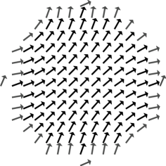
Figure 1: Magnetic structure of a spherical nanoparticle of linear size $N=15$ with $L/J=2$ for the global magnetization directed along [1,1,0], showing atoms in the plane $z=0$.

The $1/D$ surface contribution to $K_{V,{\rm eff}}$ is in accord with the picture of all magnetic atoms tightly bound by the exchange interaction whereas only the surface atoms feel the surface anisotropy. This is definitely true for magnetic films where a huge surface contribution to the effective anisotropy has been observed. The same is the case for cobalt nanoclusters of the form of truncated octahedrons jametal01 where contributions from different faces, edges, and apexes compete resulting in a nonzero, although significantly reduced, surface contribution to $K_{V,{\rm eff}}$. However, for symmetric particle shapes such as cubes or spheres, the symmetry leads to vanishing of this (first-order) contribution. In this case one has to take into account deviations from the collinearity of atomic spins that result from the competition of the SA and the exchange interaction $J$. The resulting structures (for the simplified radial SA model) can be found in Refs. dimwys9494Cobalt ; labetal02 ; dimkac0202prb (see also Fig. 1 for the NSA). In the case $L\gtrsim J$ deviations from collinearity are very strong, and it is difficult if not impossible to characterize the particle by a global magnetization suitable for the definition of the effective anisotropy. On the other hand, in the typical case $L\ll J$  the magnetic structure is nearly collinear with small deviations that can be computed perturbatively in $L/J\ll 1$. The global magnetization vector ${\bf m}_{0}$ can be used to define the anisotropic energy of the whole particle. The key point is that deviations from collinearity and thus the energies of the system are different for different orientations of ${\bf m}_{0},$ even for a particle of a spherical shape, due to the crystal lattice. For the latter the overall anisotropy per unit cell is proportional to $L^{2}/J,$ i.e., it scales with the particle’s volume.

The aim of this Letter is to illustrate this idea by calculating the second-order contribution from the NSA to the effective particle’s anisotropy for the minimal model of a magnetic nanoparticle of spherical shape cut out of a sc lattice. We will neglect the small cubic anisotropy and magnetostatic effects for the sake of transparency. The problem will be solved numerically on the lattice by minimizing the energy with the help of a damped Landau-Lifshitz equation without the precession term, with the average particle’s magnetization constrained in a desired direction. We also produce an analytical solution in the continuous limit of larger particles that will be shown to agree with the numerical solution.

We consider the nearest-neighbor form of Eq. (1) with the unique constant $L.$ For a sc lattice it reduces to

$${\cal H}_{A}=\sum_{i}{\cal H}_{Ai},\qquad{\cal H}_{Ai}=\frac{L}{2}\sum_{\alpha=x,y,z}z_{i\alpha}m_{i\alpha}^{2},$$ (2)

where $z_{i\alpha}=0,1,2$ are the numbers of available nearest neighbors of the atom $i$ along the axis $\alpha.$ One can see that the NSA is in general biaxial. For $L>0$ and $z_{i\alpha}=0<z_{i\beta}=1<z_{i\gamma}=2$ the $\alpha$-axis is the easy axis and the $\gamma$-axis is the hard axis. If the local magnetizations ${\bf m}_{i}$ are all directed along one of the crystallographic axes $\alpha,$ then the anisotropy fields ${\bf H}_{Ai}=-\partial{\cal H}_{Ai}/\partial{\bf m}_{i}$ are also directed along $\alpha$ and are thus collinear with ${\bf m}_{i}$. Hence, at least for $L\ll J,$ there are no deviations from collinearity if the global magnetization ${\bf m}_{0}$ is directed along one of the crystallographic axes. For other orientations of ${\bf m}_{0}$, the vectors ${\bf m}_{i}$ and ${\bf H}_{Ai}$ are not collinear, and the transverse component of ${\bf H}_{Ai}$ with respect to ${\bf m}_{i}$ causes a slight canting of ${\bf m}_{i}$ and thereby a deviation from the collinearity of magnetizations on different sites. This adjustment of the magnetization to the surface anisotropy leads to the lowering of energy. As we shall see, this effect is strongest for the [$\pm$1,$\pm$1,$\pm$1] orientations of ${\bf m}_{0}$. For both signs of $L$ these are easy orientations, whereas [$\pm 1,0,0],$ [$0,\pm 1,0],$ and [$0,0,\pm 1]$ are hard orientations.

We consider here explicitly spherical particles cut out of a cube with dimensions $N\times N\times N$ in the units of the atomic spacing. If an atom is within or exactly on the sphere with the diameter $D=N-1,$ it belongs to the particle. The number of atoms in the particle ${\cal N}$ approaches ${\cal N}\cong(\pi/6)(N-1)^{3}$ for $N\gtrsim 10,$ with fluctuations for smaller $N.$ Our numerical results for the magnetic energy of spherical particles as a function of the orientation of the global (average) magnetization are shown in Fig. 2. They confirm the statements of the previous paragraph.

\begin{picture}(11.0,6.0)\centerline{\hbox{\psfig{angle=-90,width=256.0748pt}}} \end{picture}

Figure 2: Reduced shifted energy of the particle for different orientations of its global magnetization, obtained from Eq. (5). These curves manifest the cubic symmetry of the effective anisotropy, see Eq. (19).

To produce Fig. 2, we use the classical Hamiltonian

$${\cal H}=-\frac{1}{2}\sum_{ij}J_{ij}{\bf m}_{i}\cdot{\bf m}_{j}+{\cal H}_{A}$$ (3)

with the nearest-neighbor exchange coupling $J$ and ${\cal H}_{A}$ of Eq. (2). To fix the global magnetization of the particle in a desired direction ${\bm{\nu}}_{0}$ (${\bm{\nu}}_{0}|=1$), we use the energy function with a Lagrange multiplier ${\bm{\lambda}}$:

$${\cal F}={\cal H}-{\cal N}{\bm{\lambda}\cdot}\left({\bm{\nu}}-{\bm{\nu}}_{0}\right),\qquad{\bm{\nu}\equiv}\frac{\sum_{i}{\bf m}_{i}}{\left|\sum_{i}{\bf m}_{i}\right|}.$$ (4)

To minimize ${\cal F},$ we solve the evolution equations

$${\bf\dot{m}}_{i} = -\left[{\bf m}_{i}\times\left[{\bf m}_{i}\times{\bf F}_{i}\right]\right],\qquad{\bf F}_{i}\equiv-\partial{\cal F}/\partial{\bf m}_{i}$$

$${\dot{\bm{\lambda}}} = {\bf\partial}{\cal F}/\partial{\bm{\lambda}=-}{\cal N}\left({\bm{\nu}}-{\bm{\nu}}_{0}\right),$$ (5)

starting from ${\bf m}_{i}={\bm{\nu}}_{0}={\bf m}_{0}$ and ${\bm{\lambda}=0,}$ until a stationary state is reached. In this state ${\bm{\nu}}={\bm{\nu}}_{0}$ and $\left[{\bf m}_{i}\times{\bf F}_{i}\right]=0,$ i.e., the torque due to the term ${\cal N}{\bm{\lambda}\cdot}\left({\bm{\nu}}-{\bm{\nu}}_{0}\right)$ in ${\cal F}$ compensates for the torque acting to rotate the global magnetizations towards the minimum-energy directions [$\pm$1,$\pm$1,$\pm$1]. Since the former torque is unphysical, this method is applicable only for a small surface anisotropy, so that both torques are small, and adding a small formal compensative torque does not strongly distort the magnetic structure.

In physical terms, the existence of the well-defined state with a given orientation of the global magnetization can be justified as follows. For $L\ll J,$ the relaxation of the magnetization splits into two stages. The first stage, adjustment of the magnetic structure to the surface anisotropy, involves energies of order $L$ and is relatively fast. The second stage, rotation of the global magnetization to the global energy minimum with the magnetic structure adjusted at any moment, involves energies of order $L^{2}/J$ and is much slower. Introducing the global-orientation constraint above eliminates the second stage of the relaxation, so that the result of the first relaxation stage is seen in pure form.

\begin{picture}(11.0,6.0)\centerline{\hbox{\psfig{angle=-90,width=256.0748pt}}} \end{picture}

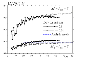
Figure 3: Differences of the particle energies between main orientations of the global magnetization vs the particle size in the scaled form for $L/J=0.1$ and 0.01. The scaling is valid for $N\lesssim J/L$, and its violation for $L/J=0.1$ is seen in the right part of the figure.

Fig. 3 shows the dependence of the normalized particle energy differences between the basic directions [001], [011], and [111]. One can see that $\Delta E/{\cal N}$ tends to a large-$N$ limit, i.e., for large linear sizes $N$ the energy differences due to the SA scale with particle’s volume $V\propto{\cal N}\sim(N-1)^{3}$. These results suggest that the problem can be solved analytically with the help of the continuous approximation for $N\gg 1.$ To this end, we replace in Eq. (2) the number of nearest neighbors of a surface atom by its average value

$$z_{i\alpha}\Rightarrow\overline{z}_{i\alpha}=2-|n_{\alpha}|/\max\left\{|n_{x}|,|n_{y}|,|n_{z}|\right\}.$$ (6)

Here $n_{\alpha}$ is the $\alpha$-component of the normal to the surface ${\bf n.}$ The surface-energy density can then be obtained by dropping the constant term and multiplying Eq. (2) by the surface atomic density $f({\bf n})=\max\left\{|n_{x}|,|n_{y}|,|n_{z}|\right\}$:

$$E_{S}({\bf m,n})=-\frac{L}{2}\left[|n_{x}|m_{x}^{2}+|n_{y}|m_{y}^{2}+\left|n_{z}\right|m_{z}^{2}\right].$$ (7)

At equilibrium, in the continuous approximation the Landau-Lifshtz equation reduces to

$${\bf m\times H}_{{\rm eff}}=0,\qquad{\bf H}_{{\rm eff}}={\bf H}_{A}+J\Delta{\bf m,}$$ (8)

where $\Delta$ is the Laplace operator and the anisotropy field

$${\bf H}_{A}=-\frac{dE_{S}}{d{\bf m}}\delta(r-R),\qquad R\equiv\frac{1}{2}\left(N-1\right).$$ (9)

For $L\ll J$ the deviations of ${\bf m(r)}$ from the homogeneous state ${\bf m}_{0}$ are small and one can linearize the problem:

$${\bf m(r)\cong m}_{0}+{\bm{\psi}}({\bf r,m}_{0}),\qquad\psi\equiv|{\bm{\psi}}|\ll 1.$$ (10)

The correction ${\bm{\psi}}$ is the solution of the internal Neumann boundary problem for a sphere

$$\Delta{\bm{\psi}}=0,\qquad\left.\frac{\partial{\bm{\psi}}}{\partial r}\right|_{r=R}={\bf f(m,n)}$$

$${\bf f}=-\frac{1}{J}\left[\frac{dE_{S}({\bf m,n})}{d{\bf m}}-\left(\frac{dE_{S}({\bf m,n})}{d{\bf m}}\cdot{\bf m}\right){\bf m}\right],$$ (11)

where ${\bf n\equiv r/}R$ and ${\bf m}$ stands for ${\bf m}_{0}$ with the index 0 dropped for transparency. $\psi$ has the form

$${\bm{\psi}}({\bf r,m})=\frac{1}{4\pi}\int_{S}d^{2}{\bf r}^{\prime}G({\bf r,r}^{\prime}){\bf f(m,n}^{\prime}{\bf)}$$ (12)

with the Green function

$$G({\bf r,r}^{\prime}) = \frac{1}{\left|{\bf r-r}^{\prime}\right|}+\frac{R}{S({\bf r,r}^{\prime})}+\frac{1}{R}\ln\frac{R^{2}}{R^{2}-{\bf r\cdot r}^{\prime}+S({\bf r,r}^{\prime})}$$

$$S({\bf r,r}^{\prime}) \equiv \sqrt{R^{4}+{\bf r}^{2}{\bf r}^{\prime 2}-2R^{2}({\bf r\cdot r}^{\prime})}.$$ (13)

One can make the estimation

$$\psi({\bf r,m})\sim RL/J\sim NL/J,\qquad|{\bf r|}=R.$$ (14)

This shows that for whatever small values of $L$ the applicability condition of our linearization method $\psi\equiv|{\bm{\psi}}|\ll 1$ will be invalidated for sufficiently large particle sizes.

Now we are prepared to calculate the magnetic energy of the nanoparticle. Dropping the trivial constant term leads to the second-order energy

$${\cal E}_{2}\cong{\cal E}_{2,V}+{\cal E}_{2,S}=\int_{V}d^{3}{\bf r}\frac{J}{2}\left(\nabla{\bm{\psi}}\right)^{2}+\int_{S}d^{2}{\bf r}\left(\frac{dE_{S}}{d{\bf m}}\cdot{\bm{\psi}}\right)$$ (15)

that is a sum of the inhomogeneous exchange and anisotropy energies. With the help of Eq. (11) this yields

$${\cal E}_{2}\cong\frac{1}{4\pi}\frac{1}{2J}\int\int_{S}d^{2}{\bf r}d^{2}{\bf r}^{\prime}G({\bf r,r}^{\prime})\Phi({\bf m},{\bf n,n}^{\prime})$$ (16)

with

$$\Phi({\bf m},{\bf n,n}^{\prime}) = \left({\bf m}\cdot\frac{dE_{S}({\bf m,n})}{d{\bf m}}\right)\left({\bf m}\cdot\frac{dE_{S}({\bf m,n}^{\prime})}{d{\bf m}}\right)$$ (17)

$$-\left(\frac{dE_{S}({\bf m,n})}{d{\bf m}}\cdot\frac{dE_{S}({\bf m,n}^{\prime})}{d{\bf m}}\right).$$

The first term in $\Phi({\bf m},{\bf n,n}^{\prime})$ can be simplified using ${\bf m}\cdot dE_{S}({\bf m,n})/d{\bf m}=2E_{S}({\bf m,n})$ following from Eq. (7). The second term in $\Phi({\bf m},{\bf n,n}^{\prime})$ is quadratic in the magnetization components and contributes only with the irrelevant term proportional to $m_{x}^{2}+m_{y}^{2}+m_{z}^{2}=1$ to the energy. Thus ${\cal E}_{2}$ simplifies to

$${\cal E}_{2}\cong\frac{1}{2\pi J}\int\int_{S}d^{2}{\bf r}d^{2}{\bf r}^{\prime}G({\bf r,r}^{\prime})E_{S}({\bf m,n})E_{S}({\bf m,n}^{\prime}),$$ (18)

that is of fourth order in the global-magnetization components $m_{\alpha}.$ Taking into account the cubic symmetry and computing numerically a double surface integral one can write the result of Eq. (18) as

$${\cal E}_{2}\cong\kappa\frac{L^{2}{\cal N}}{J_{0}}\left(m_{x}^{4}+m_{y}^{4}+m_{z}^{4}\right),\qquad\kappa=0.53465,$$ (19)

where $J_{0}=zJ=6J.$ This defines the large-$N$ asymptotes in Fig. 3 that are shown by the horizontal lines.

The analytical results above are valid for particle sizes $N$ in the range

$$1\ll N\ll J/L.$$ (20)

The lower boundary is the applicability condition of the continuous approximation. Since the surface of a nanoparticle is made of atomic terraces separated by atomic steps, each terrace and each step with its own form of NSA [see Eq. (2)], the variation of the local NSA along the surface is very strong. Approximating this variation by a continuous function according to Eq. (6) requires pretty large particle sizes $N.$ This is manifested by a slow convergence to the large-$N$ results in Fig. 3.

The upper boundary in Eq. (20) is the applicability condition of the linear approximation in ${\bf\psi},$ see Eqs. (10) and (14). For $N\gtrsim J/L$ deviations from the collinear state are strong, and the effective anisotropy of a magnetic nanoparticle cannot be introduced. The solution found above becomes invalid even for orientations of the global magnetization along the crystallographic axes where ${\bm{\psi}=0}$. In this case those surface spins close to the equatorial plane (${\bf n}\bot{\bf m}$) for $L>0$ or to the poles (${\bf n}\|{\bf m}$) for $L<0$ develop instability and turn away from ${\bf m}$ for $N\gtrsim J/L.$ Gradual disappearance of the collinear magnetic structure of a particle with increasing size stems from the “softnening” of the exchange interaction at large distances. A related phenomenon is the breakdown of the single-domain state of particles with a uniaxial bulk anisotropy with increasing size due to the magnetostatic effect.

As we have seen in Eq. (19), the contribution of the SA into the overall anisotropy of a magnetic particle scales with its volume $V\propto N^{3}\sim{\cal N}.$ This surprising result, that contradicts the initial guess on the role of the surface effects based on the ratio of the numbers of surface and volume spins $\sim 6/D$, is due to the penetration of perturbations from the surface deeply into the bulk. If a uniaxial bulk anisotropy $D_{V}$ is present in the system, perturbations from the surface will be screened at the bulk correlation length (or the domain-wall width) $\delta\sim\sqrt{J/D_{V}}.$ Then for $D\sim N\gtrsim\delta$ the contribution of the SA to the overall anisotropy will scale as the surface: ${\cal E}_{2}\sim\left(L^{2}/J\right)N^{2}\delta.$ As follows from Eq. (20), this regime requires $D_{V}\gtrsim L^{2}/J,$ i.e., the dominance of the bulk anisotropy over the SA in the overall anisotropy.

In most cases the bulk anisotropy is much smaller than the surface anisotropy for the microscopic reasons discussed at the beginning of this Letter. Then, at least for not too large particles, $N\lesssim\delta$, contributions of both anisotropies to the overall anisotropy are additive and scale as the volume. If the bulk anisotropy is cubic, both contributions have the same cubic symmetry [see Eq. (19)], and the experiment should yield a value of the effective cubic anisotropy different form the bulk valuejametal01 . For the uniaxial bulk anisotropy, the two contributions have different functional forms. Even if the bulk anisotropy is dominant so that the energy minima are realized for ${\bf m}\|{\bf e}_{z},$ the surface anisotropy makes the energy dependent on the azimuthal angle $\varphi.$ This changes the type of the energy barrier for the particle creating saddle points. The latter, in particular, strongly influences the process of thermal activation of magnetic particles garkencrocof99 .

We stress that we have calculated the second-order contribution of the Néel surface anisotropy to the effective anisotropy of a magnetic particle, and this is the only effect for symmetric particle shapes such as cubic or spherical. For small deviations from this symmetry, i.e., for weakly elliptic or weakly rectangular particles, there is a correspondingly weak first-order contribution ${\cal E}_{1}$ that adds up with our second-order contribution. For an ellipsoid with axes $a$ and $b=a(1+\epsilon)$, $\epsilon\ll 1,$ one has ${\cal E}_{1}\sim L{\cal N}^{2/3}\epsilon m_{z}^{2}$ [cf. Eq. (19)], so that

$$\frac{{\cal E}_{2}}{{\cal E}_{1}}\sim\frac{L}{J}\frac{N}{\epsilon}$$ (21)

can be large even for $L/J\ll 1.$ Whereas ${\cal E}_{1}$ scales with the particle’s surface and can be experimentally identified as a surface contribution, ${\cal E}_{2}$ scales with the volume and thus renormalizes the volume anisotropy of nanoparticles.

The Néel constant $L$ is in most cases poorly known. However, for metallic Co Ref. chubalhan94 quotes the value of SA $-1.5\times 10^{8}$ erg/cm${}^{3},$ i.e., $L\sim-10$ K. This is much smaller than $J\sim 10^{3}$ K, which makes our theory valid for particle sizes up to $N\sim J/L\sim 100,$ according to Eq. (20). For this limiting size one has ${\cal E}_{2}/{\cal E}_{1}\sim 1/\epsilon$ that is large for nearly spherical particles, $\epsilon\ll 1.$

We are indebted to R. Schilling for critical reading of the manuscript. D. G. thanks A. A. Lokshin for a valuable discussion.

References

- (1) L. Néel, J. Physique Radium 15, 255 (1954).
- (2) R. H. Victora and J. M. MacLaren, Phys. Rev. B 47, 11583 (1993).
- (3) M. Respaud, J. M. Broto, H. Rakoto, A. R. Fert, L. Thomas, B. Barbara, M. Verelst, E. Snoeck, P. Lecante, A. Mosset, J. Osuna, T. Ould Ely, C. Amiens, and B. Chaudret, Phys. Rev. B 57, 2925 (1998).
- (4) C. Chen, O. Kitakami, S. Okamoto, and Y Shimada, J. Appl. Phys. 86, 2161 (1999).
- (5) M. Jamet, W. Wernsdorfer, C. Thirion, D. Mailly, V. Dupuis, P. Mélinon, and A Pérez, Phys. Rev. Lett. 86, 4676 (2001).
- (6) D. A. Dimitrov and G. M. Wysin, Phys. Rev. B 50, 3077 (1994); Phys. Rev. B 51, 11947 (1994).
- (7) Y. Labaye, O. Crisan, L. Berger, J. P. Greneche, and J. M. D. Coey, J. Appl. Phys. 91, 8715 (2002).
- (8) M. Dimian and H. Kachkachi, J. Appl. Phys. 91, 7625 (2002); H. Kachkachi and M. Dimian, Phys. Rev. B (in print, eprint cond-mat/0109411).
- (9) D. A. Garanin, E. Kennedy, D. S. F. Crothers, and W. T. Coffey, Phys. Rev. E 60, 6499 (1999).
- (10) D. S. Chuang, C. A. Ballentine, and R. C. O’Handley, Phys. Rev. B 49, 15084 (1994).