Critical Discussion of “Synchronized Flow”,
Simulation of Pedestrian Evacuation, and
Optimization of Production Processes

Abstract

We critically discuss the concept of “synchronized flow” from a historical, empirical, and theoretical perspective. Problems related to the measurement of vehicle data are highlighted, and questionable interpretations are identified. Moreover, we propose a quantitative and consistent theory of the empirical findings based on a phase diagram of congested traffic states, which is universal for all conventional traffic models having the same instability diagram and a fundamental diagram. New empirical and simulation data supporting this approach are presented as well. We also give a short overview of the various phenomena observed in panicking pedestrian crowds relevant from the point of evacuation of buildings, ships, and stadia. Some of these can be applied to the optimization of production processes, e.g. the “slower-is-faster effect”.

1 Freeway Traffic: “Synchronized flow”, “Pinch Effect”, and Measurement Problems

1.1 What is new about “synchronized flow?”

Congested traffic has been investigated for many decades because of its complex phenomenology. Therefore, Kerner and Rehborn have removed the data belonging to wide moving jams (see MLC and TSG in Figs. 9 and 10) and found found that the remaining data of congested traffic data still displayed a wide and two-dimensional scattering KerRe96b , see Fig. 4(c). By mistake (see Figs. 1, 4(c), and Sec. 1.2), they concluded that all models assuming a fundamental diagram were wrong and defined a new state called “synchronized flow” (“synchronized” because of the typical synchronization among lanes in congested traffic, see Fig. 2(a), and “flow” because of flowing in contrast to standing traffic in fully developed jams). Since then, Kerner suggests to classify three phases: (1) free flow, (2) “synchronized flow”, and (3) wide moving jams (i.e. moving localized clusters whose width in longitudinal direction is considerably higher than the width of the jam fronts). In some applied empirical studies, however, Kerner et al. additionally distinguish a fourth state of stop-and-go traffic FOTO ; KerReAl00 .

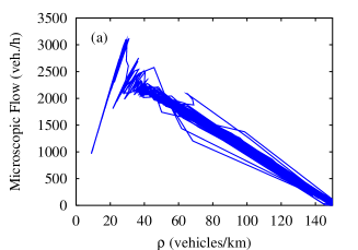
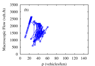
Figure 1: (a) Flow-density relation for narrow moving jams simulated with a microscopic traffic model. (b) The aggregated (1-minute) data corresponding to the narrow moving jams displayed in (a) show a wide scattering and erratic movement in the flow-density plane. By mistake, this is used to characterize “synchronized flow”.

Free flow is characterized by the average desired velocity $V_{0}$ and, therefore, by a strong correlation and quasi-linear relation $Q\approx\rho V_{0}$ between the local flow $Q$ and the local density $\rho$ NeubSaScSc99 . It is also well-known that wide moving jams propagate with constant form and (phase) velocity $C\approx-13$km/h MikaKrYu69 ; KerRe96a ; CasMa99 . Kerner found that this propagation is not affected by bottlenecks or the presence of “synchronized flow”. Moreover, he showed that the outflow $Q_{\rm out}$ from wide jams is a self-organized traffic constant as well KerRe96a ; Kerner1 . In contrast to wide moving jams, the flow inside of “synchronized flow” remains finite, and its downstream front is normally fixed at the location of some bottleneck, e.g. an on-ramp. Therefore, “synchronized flow” basically agrees with previous observations of queued or congested traffic (see, e.g., Refs. Per86 ; Bank90 ; Bank91a and the references therein). In his patent KerKirReh , Kerner applies the queuing theory himself, which goes back to the fluid-dynamic traffic model by Lighthill and Whitham LighWh55 .

The synchronization of the average velocities among neighboring lanes has been already described by Koshi et al. KosIwOh83 (but see also Refs. MikaKrYu69 ; EdiFo58 ; ForMuSi67 ). It is true on a macroscopic level for all forms of congested traffic including wide moving jams. Simulations have shown that this is a result of lane changes Lee3LeKi98 , while the assumed reduction in the lane changing rate KerRe97 occurs only after the speeds in neighboring lanes have been successfully balanced ShvHe99 . On a microscopic scale, over-taking maneuvers continue to exist almost at all densities HelHu98 , see Figs. 2(b), (c). Nevertheless, the probability of lane changes drops considerably with increasing density, when most of the road is used up by the vehicles’ safety headways HelHu98 , but not in the postulated $Z$-shaped way Kerner3 . Due to the reduced opportunities for overtaking and the related bunching of vehicles, the velocity variance goes down with increasing density as well KerRe97 ; Hel97a ; Hel97c .

Figure 2: (a) The difference of the average velocity in the left and the right lane vanishes at densities above 30 vehicles per kilometer, corresponding to a macroscopic synchronization of the speeds Hel97a . (b), (c) The difference in the empirically determined velocities of cars and trucks, however, show that overtaking maneuvers continue to exist even at higher densities HelHu98 .

The transition between free and congested traffic is of hysteretic nature, i.e. the inverse transition occurs at a lower density and a higher average velocity. This has been known for a long time TreitMy74 ; Pay84 ; Hal187 . Kerner specifies that the transition is usually caused by a localized and short perturbation of traffic flow that starts downstream of the on-ramp and propagates upstream with a velocity of about $-13$ km/h. As soon as the perturbation passes the on-ramp, it triggers the breakdown which spreads upstream in the course of time. The congested state can then persist for several hours KerRe97 .

Moreover, Kerner and Rehborn distinguish three types of “synchronized flow” KerRe96b , which may be short-lived: (i) Stationary and homogeneous states where both the average speed and the flow rate are stationary (see, e.g., also Refs. Hal1Ag91 ; PerYaBr98 ; Wes98 . Later on, we will these “homogeneous congested traffic” (HCT) HelHeTr99 .
(ii) States where only the average vehicle speed is stationary, named “homogeneous-in-speed states” (see also Refs. Ker98b ; Lee3LeKi00 ). We interpret this state as “recovering traffic” Review , as it bears several signatures of free traffic and mostly appears downstream of bottlenecks with congested traffic.
(iii) Non-stationary and non-homogeneous states (see also Refs. Ker98b ; CasBe99 ; TreHeHe00 ). For these, we will use the term “oscillating congested traffic” (OCT) HelHeTr99 .
At least types (i) and (iii) are characterized by a considerably scattering and erratic change of the flow-density data, the various sources of which will be addressed in the following subsection. Continuous transitions between these types are probably the reason for the so-called “pinch effect” Ker98a , see Fig. 3(a):

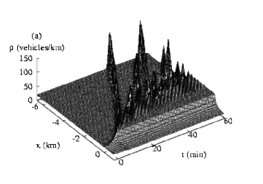
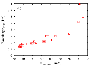
Figure 3: (a) Simulation of the pinch effect with a deterministic microscopic model showing stable traffic at low and high densities, linearly unstable traffic at medium densities, and metastable traffic in between. The spatio-temporal density plot illustrates the breakdown to homogeneous congested traffic (HCT) upstream of a bottleneck, emerging oscillating congested traffic (OCT) further upstream, and a few stop-and-go waves (TSG) emanating from this region. The conditions for this spatial coexistence of congested traffic states are as follows Review ; TreHe99b : The density in the congested region immediately upstream of the bottleneck should be in the linearly unstable, but convectively stable range, where perturbations are convected away in upstream direction Mann90 ; CrosHo93 . In this case, traffic flow will appear stationary and homogeneous close to the bottleneck, but small perturbations will grow as they propagate upstream in the congested region starting at the bottleneck. If the perturbations propagate faster than the congested region expands, they will reach the area of free traffic upstream of the bottleneck. During rush hours, it is quite likely that this free flow is in the metastable range between the free and linearly unstable density region. Consequently, sufficiently large perturbations can trigger the formation of jams, which continue travelling upstream, while small perturbations are absorbed. (b) The wavelength (average distance between density maxima) determined from (a) qualitatively displays the empirical increase with the vehicle velocity observed by Kerner Ker98a .

Upstream of a section with homogeneous congested traffic close to a bottleneck, there is a so-called “pinch region” characterized by the spontaneous birth of small and narrow density clusters, which are growing while they travel further upstream. Wide moving jams are eventually formed by the merging or disappearance of narrow jams, in which the cars move slower than in wide jams Ker98a . Once formed, the wide jams seem to suppress the occurence of new narrow jams in between. Similar findings were already reported by Koshi et al. KosIwOh83 , who observed that “ripples of speed grow larger in terms of both height and length of the waves as they propagate upstream”.

1.2 Wide scattering of congested flow-density data

The collection and evaluation of empirical freeway data is a subject with often underestimated problems. To make reliable conclusions, in original investigations one should specify (i) the measurement site and conditions (including applied control measures), (ii) the sampling interval, (iii) the aggregation method, (iv) the statistical properties (variances, frequency distributions, correlations, survival times of traffic states, etc.), (v) data transformations, (vi) smoothing procedures, and the respective dependencies on them.

Figure 4: (a) The empirical truck fraction varies considerably in the course of time. (b) The time headways of long vehicles (“trucks”) are on average much higher than those of short vehicles (“cars”). (c)-(e) Assuming a fundamental diagram for cars (solid line), a separate one for trucks (dashed line), weighting them according to the measured truck fraction, and using empirical boundary conditions allows to reproduce the observations in a (semi-)quantitatively way TreHe99a : Free traffic (at low densities) is characterized by a (quasi-)one-dimensional curve. (c) Data of congested traffic upstream of a bottleneck are widely scattered in a two-dimensional area. (d) Immediately downstream of the bottleneck, one observes homogeneous-in-speed states reflecting recovering traffic. (e) Further downstream the data points approach the curve describing free traffic. Dark symbols correspond to empirical one-minute data, light ones to corresponding simulation results.

The measurement conditions include ramps and road sections with their respective in- and outflows, speed limits, gradients, and curves with the respectively related capacities, furthermore weather conditions (like rain, ice, blinding sun, etc.), presence of incidents (including the opposite driving direction), and other irregularities such as road works, which may trigger a breakdown of traffic flow. Moreover, one should evaluate the long vehicles (“trucks”) separately, as their proportion varies significantly, see Fig. 4(a). This can explain a considerable part of the wide scattering of congested traffic TreHe99a , see Figs. 4(c), (d). Presently, this explanation is still the only one for this observation that has been quantitatively checked with empirical data. Note that a considerable variation of the time headways is also observed among cars, see Fig. 4(b). This is partly due to different driver preferences and partly due to the instability of traffic flow, see Fig. 5(a). While vehicle platoons with reduced time headways imply an increase of the flow with growing density, a reduction in vehicle speeds is usually related with a decrease. According to Banks Bank99 , this can account for the observed erratic changes of the flow-density data. We support this interpretation.

Figure 5: (a) The measured oscillations of the clearance and the relative velocity Hoe72 indicate an instability in the car-following behavior HelTi98 . (b) The empirical standard deviation $\sqrt{\theta(t)}$ of vehicle velocities divided by the average velocity $V(t)$ is particularly large during the rush hour, where traffic flow is congested and unstable Review ; Tilch01 .

The strong variations of traffic flows imply that all measurements of macroscopic quantities should be complemented by error bars (see, e.g., Ref. Hal1AlGu86 ). Due to the relatively small “particle” numbers behind the determination of macroscopic quantities, the error bars are actually quite large. Hence, many temporal variations are within one error bar, when traffic flow is unstable, see Fig. 5(b). It is, therefore, very questionable whether it is possible to empirically prove the existence of small perturbations triggering a breakdown of traffic flow KerRe97 or of the “birth” and merging of narrow density clusters in the “pinch region” Ker98a . At least, this would require a thorough statistical support. Consequently, we deny that such kind of data are presently suited as starting point for the development of new models KerMic or traffic theories Kerner3 . There is a considerable risk of overinterpreting particular (possibly statistical) features of the data recorded at special freeway sections and to construct new models that merely simulate what has been incorporated by means of the model assumptions. In fact, the only reason why we believe in the correctness of these observations is the existence of plausible deterministic traffic models reproducing these hard-to-see effects without any special assumptions or extensions (see Fig. 3 and Refs. Lee3LeKi98 ; TreHe99b ; HelTr98a ).

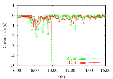
Figure 6: The covariance between headways $d_{\alpha}$ and inverse velocities $1/v_{\alpha}$ shows significant deviations from zero in congested traffic, while it approximately vanishes in free flow, compare Fig. 5(b). Even after traffic has recovered, there seem to remain weak correlations between headways and vehicle speeds for a considerable time. These are probably a reminiscence of congestion due to platoons which have not fully dissolved Review ; Tilch01 .

Because of the above mentioned problems, we would like to call for more refined measurement techniques, which are required for more reliable data. These must take into account correlations between different quantities, as is pointed out by Banks Bank95 .

For example, approximating the vehicle headways by $d_{\alpha}=v_{\alpha}\Delta t_{\alpha}$ (where $v_{\alpha}$ is the velocity and $\Delta t_{\alpha}$ the time headway of vehicle $\alpha$) and determining arithmetic multi-vehicle averages $\langle\dots\rangle$ at a fixed location, one obtains for the inverse vehicle flow

$$\frac{1}{Q}=\langle\Delta t_{\alpha}\rangle=\left\langle\!\frac{d_{\alpha}}{v_{\alpha}}\!\right\rangle=\langle d_{\alpha}\rangle\left\langle\!\frac{1}{v_{\alpha}}\!\right\rangle+\mbox{cov}\left(\!d_{\alpha},\frac{1}{v_{\alpha}}\!\right)\,.$$ (1)

Herein, $\mbox{cov}(d_{\alpha},1/v_{\alpha})$ denotes the covariance between the headways $d_{\alpha}$ and the inverse velocities $1/v_{\alpha}$, which is negative and particularly relevant at large vehicle densities, as expected (see Fig. 6). Defining the local density $\rho$ by

$$\rho=1/\left\langle d_{\alpha}\right\rangle$$ (2)

and the average velocity $V$ via

$$\frac{1}{V}=\left\langle\frac{1}{v_{\alpha}}\right\rangle\,,$$ (3)

we obtain the fluid-dynamic flow relation

$$Q=\rho V$$ (4)

by the conventional assumption $\mbox{cov}(d_{\alpha},1/v_{\alpha})=0$. This, however, overestimates the density systematically, since the covariance tends to be negative due to the speed-dependent safety distance of vehicles. In contrast, the common method of determining the density via $Q/\langle v_{\alpha}\rangle$ systematically underestimates the density Review ; TilHe00 . Consequently, errors in the measurement of the flow and the density due to a neglection of correlations partly account for the observed scattering of flow-density data in the congested regime.

A similar problem occurs when the density is determined via the time occupancy of a certain cross section of the road. Considering that $\Delta t_{\alpha}=T_{\alpha}+l_{\alpha}/v_{\alpha}$, where $T_{\alpha}$ is the (netto) time clearance and $l_{\alpha}$ the length of vehicle $\alpha$, we have the relation

$$\rho=\rho_{\rm max}\frac{\langle l_{\alpha}/v_{\alpha}\rangle}{\langle\Delta t_{\alpha}\rangle}=\rho_{\rm max}Q\langle l_{\alpha}/v_{\alpha}\rangle=\frac{Q}{\langle l_{\alpha}\rangle}\langle l_{\alpha}/v_{\alpha}\rangle\,,$$ (5)

where $\rho_{\rm max}=1/\langle l_{\alpha}\rangle$ is the maximum density and $\langle l_{\alpha}\rangle$ the average vehicle length. For a finite detector length $L_{D}$, we have to replace $l_{\alpha}$ by $l_{\alpha}+L_{D}$ Review ; May90 . The formula $1/V=\langle l_{\alpha}/v_{\alpha}\rangle/\langle l_{\alpha}\rangle$ for the average velocity results in the correct expression $1/V=\langle 1/v_{\alpha}\rangle$ only, if the individual vehicle lengths and velocities are not correlated, which is usually not the case.

1.3 A quantitative theory of congested traffic states

When Kerner started to question all traffic models with a fundamental diagram, physicists were used to simulate traffic in closed systems with periodic boundary conditions. With the Kerner-Konhäuser model, it was possible to produce free traffic, emergent stop-and-go waves, and triggered wide moving jams Kuh84a ; Kuh91a ; KerKo94 . However, attempts to simulate “synchronized flow” failed even when small ramp flows were added to the system. They resulted in what we call a pinned localized cluster (PLC) located at the on-ramp KerPLC (see Figs. 9 and 10). Because of the sensitivity of the model and problems with the treatment of open systems, it was not possible to simulate open systems with considerable ramp flows. Other independent studies for periodic systems with localized bottlenecks produced either homogeneous vehicle queues (HCT) or oscillating congested traffic (OCT) Lee3LeKi98 ; MunHsLa71 ; Phi77 ; Cre79 ; MakNaToMi81 ; ChuHu94 ; EmmRa95 ; CsaVi94 ; Hil95 ; KlaKuWe96 ; Naga97c , but at that time nobody could make sense of these apparently inconsistent findings. This situation changed, when Helbing et al. derived a phase diagram of congested traffic states. They managed to simulate a macroscopic traffic model with open boundary conditions even in extreme situations and investigated a freeway stretch with a single ramp HelHeTr99 . Instead of the densities, they identified the main flow on the freeway and the on-ramp flow as the suitable control parameters for on open system and varied them systematically. In this way, they found that a perturbation could trigger different kinds of congested traffic states. Moreover, the boundaries separating different states could be related to the instability diagram for homogeneous freeways and other characteristic quantities HelHeTr99 . For this reason, they concluded that the phase diagram should be qualitatively the same, i.e. universal, for all microscopic, mesoscopic, or macroscopic traffic models having the same instability diagram. This has been supported in the meantime HelHeTr99 ; TreHeHe00 ; Lee3LeKi99 . Apart from this, the phase diagram of traffic models with different instability diagrams can be directly derived Review . Generalizations to other kinds of bottlenecks (e.g. gradients) have been developed as well TreHeHe00 .

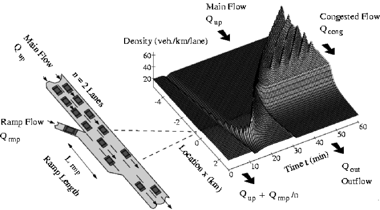
Figure 7: Negative perturbation triggering oscillating congested traffic. When the traffic density has sufficiently increased to reach the metastable regime, the “negative” perturbation will be amplified if it only exceeds the critical amplitude. While it is small, it will move downstream with the vehicles, so one could hope it would pass the bottleneck and leave the system. However, when the density wave grows larger, it will reduce its speed and even change its propagation direction. Once it is fully developed, it moves upstream with constant velocity, since vehicles leave the jam at the downstream front, while new ones join it at the upstream front. Hence, the perturbation returns to the bottleneck (see Fig. 8 for this “boomerang effect”), and it triggers a breakdown of traffic, when it passes the bottleneck in upstream direction, as it thereby reduces the effective capacity to $Q_{\rm out}$ Review ; HelTr98a ; PhysikBl .

In the following, we will sketch the basic ideas behind the phase diagram of congested traffic states (for a more detailed discussion see Ref. Review ). Let us assume our traffic model has a fundamental diagram

$$Q_{\rm f}(\varrho)=\varrho V_{\rm f}(\varrho)$$ (6)

describing the relation between the vehicle flow $Q$, the spatially averaged density $\varrho$, and the average velocity $V$ in homogeneous and stationary traffic. (The flow-density relation of emergent stop-and-go waves is characterized by a linear relation, i.e. it looks differently KerKo94 .) Moreover, let us assume the model has ranges of stable traffic flow at small and high densities, a range of linearly unstable traffic flow at medium densities, and ranges of metastable traffic flow in between. This kind of instability diagram is, for example, found for the macroscopic model used by Kühne, Kerner and Konhäuser, or Lee et al. Lee3LeKi98 ; Kuh84a ; KerKo94 , for the microscopic optimal velocity model BandHaNaNaShSu95 , for the non-local gas-kinetic-based traffic model TreHeHe99 , or the microscopic intelligent driver model TreHeHe00 (among which the first two models are rather sensitive to parameter variations, but the latter two are quite robust).

In contrast to circular freeways, emergent “phantom traffic jams” are not typical for open homogeneous freeway stretches, as it is normally impossible to reach the linearly unstable density regime by feeding in vehicles at the upstream boundary. This is in agreement with empirical observations Kerner4 . Most cases of traffic congestion on an $n$-lane freeway are observed upstream of on-ramps or other bottlenecks. They can be triggered by perturbations significantly below the theoretical capacity, as soon as the sum of the upstream freeway flow $Q_{\rm up}$ and the on-ramp flow $\Delta Q=Q_{\rm rmp}/n$ per lane exceeds the outflow $Q_{\rm out}$ from congested traffic: If a disturbance leads to temporary congestion, the drivers must accelerate again and suffer some time delay, which reduces the capacity to $Q_{\rm out}$. Therefore, the following vehicles will queue up, and the temporary perturbation grows to form a persistent kind of congestion. The initial perturbation can even be a temporary reduction of the traffic flow and/or vehicle density, which can be caused by temporal variations of the traffic volume or even by vehicles leaving the freeway at some off-ramp DagCaBe99 ; PhysikBl , see Fig. 8.

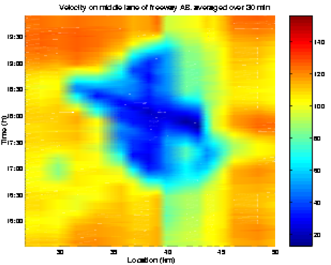
Figure 8: The wide moving jam left of kilometer 43 starts with a “boomerang effect” and travels through the “synchronized” congested traffic flow left of kilometer 41 (dark area). (Reproduction with kind permission of Rudolf Sollacher, Siemens AG, Munich.)

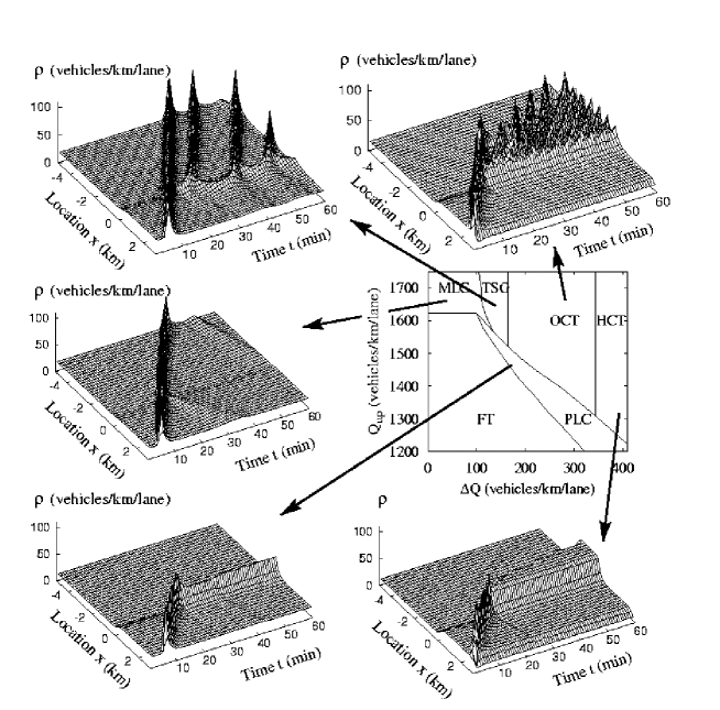
Figure 9: Simulated representatives (density-over-space-and-time plots) of the different congested traffic states, which were triggered by a big perturbation travelling upstream. Center right: Phase diagram of the traffic states as a function of the (upstream) traffic volume $Q_{\rm up}$ on the freeway and the strength $\Delta Q$ of a bottleneck at location $x=0$ km, e.g. an on-ramp with inflow $\Delta Q$ per freeway lane.

If the total traffic volume $Q_{\rm tot}=(Q_{\rm up}+\Delta Q)$ is greater than the dynamic capacity $Q_{\rm out}$, we will automatically end up with a growing vehicle queue upstream of the on-ramp. The traffic flow $Q_{\rm cong}$ resulting in the congested area normally gives, together with the inflow $\Delta Q$, the outflow $Q_{\rm out}$, i.e. $Q_{\rm cong}=(Q_{\rm out}-\Delta Q)$ (but see the footnote on p. 1111 of Ref. Review for exceptions). One can distinguish the following cases HelHeTr99 ; TreHeHe00 ; Review (see Fig. 9): If the density $\varrho_{\rm cong}$ associated with the flow $Q_{\rm cong}=Q_{\rm f}(\varrho_{\rm cong})$ is stable, we find homogeneous congested traffic (HCT) such as typical traffic jams during holiday seasons. For a smaller on-ramp flow $\Delta Q$, the congested flow $Q_{\rm cong}$ is linearly unstable, and we either find oscillating congested traffic (OCT) or triggered stop-and-go traffic (TSG), which often emerges from a spatial sequence of homogeneous and oscillating congested traffic (so-called “pinch effect” Ker98a ). In contrast to OCT, stop-and-go traffic is characterized by a sequence of moving jams, between which traffic flows freely. Each traffic jam triggers the next one by inducing a small perturbation at the ramp, which propagates downstream as long as it is small, but turns back when it has grown large enough (“boomerang effect”, cf. Figs. 7 to 10). This, however, requires the downstream traffic flow to be linearly unstable. If it is metastable instead (when the traffic volume is further reduced), a traffic jam will usually not trigger a growing perturbation. In that case, one finds either a single moving localized cluster (MLC), or a pinned localized cluster (PLC) at the location of the ramp. The latter requires the traffic flow in the upstream section to be stable, so that no traffic jam can survive there. Finally, for sufficiently small traffic volumes, we find free traffic (FT), as expected.

The different congested traffic states found in the microsimulations (as displayed in Fig. 9) could all be identified in real traffic data (see Fig. 10 for some examples). Moreover, according to our first investigation results, the traffic patterns observed on the German freeway A5 near Frankfurt have a typical dependence on the respective weekday and are even quantitatively consistent with the phase diagram (see Fig. 10). Of course, the empirically measured patterns look less regular, as the simulation results displayed in Fig. 9 are for a deterministic model with identical vehicle parameters.

Figure 10: Empirical examples of triggered stop-and-go traffic (TSG), oscillating congested traffic (OCT), and pinned localized clusters (PLC), and the location of the empirical data points in the phase diagram for the German freeway A5 near Frankfurt.

We will now reply to some criticism and misunderstandings: (1) Although the phase diagram and the congested traffic states have been derived for identical driver-vehicle units and one bottleneck only, many observations already fit very well into this scheme. If several bottlenecks are present, the situation becomes more complicated, but can be addressed by similar methods. In such cases, we may find the spatial coexistence of states such as OCT and PLC, transitions between different states, extended congested traffic states (HCT, OCT, or TSG) with a fixed upstream front, and other phenomena. The phenomenon of multistability and coexisting states is, by the way, already found for the case of one single bottleneck (see Ref. Lee3LeKi99 and Fig. 8 in Ref. TreHeHe00 ). (2) Because of a certain “penetration depth” TreHeHe00 , MLC states can propagate through small areas of stable traffic. (3) The variation and scattering of the flow-density data is well reproduced, if different driver-vehicle types are distinguished (and overtaking maneuvers are taken into account). (4) The “pinch effect” does not correspond to a transition between different phases (HCT, OCT, and TSG) in the course of time, but it corresponds to a certain area in the phase diagram, where the congested flow is convectively stable but linearly unstable (not shown). The empirically observed increase of the vehicle velocity in “synchronized flow” with the average oscillation wavelength Ker98a is qualitatively well reproduced, see Fig. 3(b). (5) The flow downstream of congested traffic can exceed the dynamical capacity $Q_{\rm out}$, if vehicles can enter the freeway via the ramp downstream of the congestion front Kerner3 . This is practially relevant for particularly long on-ramps like freeway intersections (see Footnote on p. 1111 of Ref. Review ).

2 Pedestrian Evacuation

The topics of pedestrian traffic and evacuation of buildings, stadia, and ships have recently attracted great interest among traffic scientists. Here, we will give a short overview only, as there are several detailed reviews available (see Refs. Hel97a ; Review ; HelMo2FaBo00 ; SchSh01 ; PED ). We will focus on the social-force model of pedestrian dynamics which describes the different competing motivations of pedestrians by separate force terms. It has the following advantages:
(1) The social-force model takes into account the flexible usage of space (i.e. the compressibility of the crowd), but also the excluded volume and friction effects which play a role at extreme densities. (2) The model assumptions are simple and plausible. Virtual fields BurKlaSchZi01 or other questionable model ingredients are not necessary to obtain realistic results. (3) There are only a few model parameters to calibrate. (4) The model is robust and naturally reproduces many different observations without modifications of the model. (5) Nevertheless, it is easy to consider individual differences in the behavior, and extensions for more complex problems such as trail formation Hel97a ; HelMo2FaBo00 ; HelKe1Mo97 are possible.

Figure 11: (a) Formation of lanes in initially disordered pedestrian crowds with opposite walking directions and small noise amplitudes $\eta_{i}$ (after Review ; PED ; HelFaVi00a ; cf. also HelMo295 ; HelVi99 ). White disks represent pedestrians moving from left to right, black ones move the other way round. (b) For sufficiently high densities and large fluctuations, we observe the noise-induced formation of a crystallized, “frozen” state (after Review ; HelFaVi00a ).

For normal, “relaxed” situations with small fluctuation amplitudes, our microsimulations of counterflows in corridors reproduce the empirically observed formation of lanes consisting of pedestrians with the same desired walking direction Review ; HelFaVi00a ; HelMo295 ; HelVi99 , see Fig. 11(a). If we do not assume periodic boundary conditions, these lanes are dynamically varying (see the Java applet at www.helbing. org/Pedestrians/ Corridor.html). Their number depends on the width of the street HelMo295 , on pedestrian density, and on the noise level. Interestingly, one finds a noise-induced ordering HelPl00 : Compared to small noise amplitudes, medium ones result in a more pronounced segregation (i.e., a smaller number of lanes). Large noise amplitudes lead to a “freezing by heating” effect characterized by a breakdown of “fluid” lanes and the emergence of “solid” blockages HelFaVi00a , see Fig. 11(b). Note that our model can explain lane formation even without assuming asymmetrical interactions or attraction effects HelFaVi00a ; HelMo295 ; HelVi99 . It is an optimal self-organization phenomenon HelVi99 resulting from the combination of driving and repulsive forces. The same model also reproduces the observed oscillations of the flow direction at bottlenecks Review ; PhysikBl ; HelMo295 without the need of a virtual “floor field” Scha01 ; BurKirKlaSchZi01 . Cellular automaton Java applets from 1998 are available in the internet to visualize these phenomena (see www.helbing.org/Pedestrians/ Corridor.html, Door.html). They are based on a discretization of the social force model that can be viewed as a discrete two-dimensional optimal velocity model Bolay98 . For other cellular automata see Ref. SchSh01 ; BlueAd98 ; FukIs99a ; MuraIrNa99 ; KluMeWaSc00 .

“Freezing by heating” is one of the phenomena observed in crowd stampedes. Another one is the “faster-is-slower effect” (or “slower-is-faster effect”) HelFaVi00b . It can trigger a “phantom panic” HelFaVi00b and is caused by arching and clogging at bottlenecks like exits, see Fig. 12(a).

Figure 12: (a)When the desired velocity $v_{0}$ is too high (e.g. in panic situations), pedestrians come so close to each other, that their physical contacts cause the build up of pressure and obstructing friction effects, which results in temporary arching and clogging (for online Java simulations see http://angel.elte.hu/$\tilde{\hphantom{n}}$panic/). (b) This is related with an inefficient and irregular outflow, while the outflow is regular for small enough desired velocities ($v_{0}\leq 1.5$ m/s) Review ; PED ; HelFaVi00b . (c) In panicking crowds, high pressures build up due to physical interactions. This can injure people (black disks), who turn into obstacles for other pedestrians trying to leave PED . (d) A column in front of the exit (large black disk) can avoid injuries by taking up pressure from behind. It can also significantly increase the outflow PED . In large exit areas used by several hundret people, several randomly placed columns are needed to subdivide the crowd and the pressure. An asymmetric configuration of the columns is most efficient, as it avoids equilibria of forces which may temporarily stop the outflow. (See http://angel.elte.hu/$\tilde{\hphantom{n}}$panic/ for online Java simulations.)

The underlying reason is the friction effect occuring in dense crowds, if the desired velocity is so high that pedestrians have physical interactions. In these situations, extreme pressure can build up in the crowd, and people may be crushed or trampled, in this way turning into obstacles for other fleeing people, see Fig. 12(c). These dangerous pressures can be reduced by columns, when suitably placed in front of the exits, see Fig. 12(d). Thereby, the number of injuries can be significantly reduced, and the outflows are considerably increased (see the Java applets at http://angel.elte.hu/$\tilde{\hphantom{n}}$panic/).

Not only bottlenecks are dangerous in panic situations, but also widenings HelFaVi00b . These can reduce the efficiency of leaving, see Figs. 13(a), (b). Another problem is herding behavior, as it is responsible for an inefficient use of available exits Review ; HelFaVi00b , see Figs. 13(c), (d).

Figure 13: (a), (b) Drop of the efficiency of leaving in corridors with widenings PED ; HelFaVi00b . (c), (d) Herding behavior of panicking pedestrians in a smoky room (black), leading to an inefficient use of available escape routes PED ; HelFaVi00b . (Online Java simulations of this effect are provided at http://angel.elte.hu/$\tilde{\hphantom{n}}$panic/.)

3 Summary and Application to Optimal Production Processes

Nowadays, most aspects of traffic dynamics have been understood on the basis of self-driven many-particle models. The observed phenomena can be (semi-)quantitatively reproduced by simulations using measured boundary conditions TreHeHe00 . Moreover, a universal phase diagram of congested traffic states for freeway sections with one bottleneck has been found, and the generalization to more complex situations is straightforward. The reproduction of fine details, however, will require a more detailed measurement of the interactive vehicle dynamics and the consideration of psychological aspects. Although these may also be described in a mathematical way KerMic , it will be hardly possible to prove or disprove the corresponding models, i.e. the criteria demanded in the natural sciences would have to be relaxed. A more promising research direction is the modelling and optimization of production processes. For example, applying the knowledge of the “slower-is-faster effect” to the treatment times in a series of production steps, we were able to increase the throughput of production processes in a major Chip factory by up to 39% Fasold .

Figure 14: (a) Gantt diagramm illustrating the treatment times in different modules, corresponding to different production steps. The limiting factor for increasing the throughput is the transport module. (b) Applying the knowledge of the “slower-is-faster effect” to the treatment times, we were able to increase the throughput of some production processes in a major Chip factory by 33% or even more Fasold .

Many conclusions from traffic models are relevant for the organization of societies, administrations, companies, production processes, and so on, as the basic model ingredients agree: (1) The system consists of a large number of similar units/entities (individuals, pedestrians, cars, boxes, …). (2) The units are externally or internally driven, i.e. there is some energy input, e.g., they can move. (3) Units are non-linearly interacting, i.e. under certain conditions, small variations can have large effects. The system behavior is dominated by interactions rather than by the boundary conditions (the external control). (4) There is a competition for resources such as time (slots), space, money. (5) Each unit has a certain extension in space or time. (6) When units come too close, they have frictional effects and obstruct each other.

References

- (1) B. S. Kerner, H. Rehborn: Phys. Rev. E 53, R4275 (1996)
- (2) B. S. Kerner, H. Rehborn, M. Aleksic, A.Haug, R. Lange: Straßenverkehrstechn. 10, 521 (2000)
- (3) B. S. Kerner, H. Rehborn, M. Aleksic: in Traffic and Granular Flow ’99, edited by D. Helbing, H. J. Herrmann, M. Schreckenberg, and D. E. Wolf (Springer, Berlin 2000), pp. 339–344
- (4) L. Neubert, L. Santen, A. Schadschneider, M. Schreckenberg: Phys. Rev. E 60, 6480 (1999)
- (5) H. S. Mika, J. B. Kreer, L. S. Yuan: Highw. Res. Rec. 279, 1 (1969)
- (6) B. S. Kerner, H. Rehborn: Phys. Rev. E 53, R1297 (1996)
- (7) M. J. Cassidy, M. Mauch: Transpn. Res. A 35, 143 (2001)
- (8) B. S. Kerner, S. L. Klenov, P. Konhäuser: Phys. Rev. E 56, 4200 (1997)
- (9) B. N. Persaud: ‘Study of a freeway bottleneck to explore some unresolved traffic flow issues’, Ph.D. thesis, University of Toronto (1986)
- (10) J. H. Banks: Transpn. Res. Rec. 1287, 20 (1990)
- (11) J. H. Banks: Transpn. Res. Rec. 1320, 83 (1991)
- (12) B. S. Kerner, H. Kirschfink, H. Rehborn: German Patent DE 196 47 127.3; US Patent US 5,861,820 (1999)
- (13) M. J. Lighthill, G. B. Whitham: Proc. Roy. Soc. London, Ser. A 229, 317 (1955)
- (14) M. Koshi, M. Iwasaki, I. Ohkura: In: Proceedings of the 8th International Symposium on Transportation and Traffic Flow Theory, ed. by V. F. Hurdle, E. Hauer, G. N. Stewart (University of Toronto, Toronto, Ontario 1983) pp. 403
- (15) L. C. Edie, R. S. Foote: High. Res. Board Proc. 37, 334 (1958)
- (16) T. W. Forbes, J. J. Mullin, M. E. Simpson: In: Proceedings of the 3rd International Symposium on the Theory of Traffic Flow, ed. by L. C. Edie (Elsevier, New York, N. Y. 1967) pp. 97
- (17) H. Y. Lee, H.-W. Lee, D. Kim: Phys. Rev. Lett. 81, 1130 (1998)
- (18) B. S. Kerner, H. Rehborn: Phys. Rev. Lett. 79, 4030 (1997)
- (19) V. Shvetsov, D. Helbing: Phys. Rev. E 59, 6328 (1999)
- (20) D. Helbing, B. A. Huberman: Nature 396, 738 (1998)
- (21) B. S. Kerner: Networks and Spatial Economics 1, 35 (2001)
- (22) D. Helbing: Verkehrsdynamik (Springer, Berlin 1997)
- (23) D. Helbing: Phys. Rev. E 55, 3735 (1997)
- (24) J. Treiterer, J. A. Myers: In: Proceedings of the 6th International Symposium on Transportation and Traffic Theory, ed. by D. Buckley (Reed, London 1974) pp. 13
- (25) H. Payne: Transpn. Res. Rec. 971, 140 (1984)
- (26) F. L. Hall: Transpn. Res. A 21, 191 (1987)
- (27) F. L. Hall, K. Agyemang-Duah: Transpn. Res. Rec. 1320, 91 (1991)
- (28) B. Persaud, S. Yagar, R. Brownlee: Transpn. Res. Rec. 1634, 64 (1998)
- (29) D. Westland: In: Proceedings of the 3rd International Symposium on Highway Capacity, ed. by R. Rysgaard (Road Directorate, Denmark 1998) pp. 1095
- (30) D. Helbing, A. Hennecke, M. Treiber: Phys. Rev. Lett. 82, 4360 (1999)
- (31) B. S. Kerner: In: Proceedings of the 3rd International Symposium on Highway Capacity, ed. by R. Rysgaard (Road Directorate, Denmark 1998) Vol. 2, pp. 621
- (32) H. Y. Lee, H.-W. Lee, D. Kim: Phys. Rev. E 62, 4737 (2000)
- (33) D. Helbing: Reviews of Modern Physics 1067, 1141
- (34) M. J. Cassidy, R. L. Bertini: Transpn. Res. B 33, 25 (1999)
- (35) M. Treiber, A. Hennecke, D. Helbing: Phys. Rev. E 62, 1805 (2000)
- (36) B. S. Kerner: Phys. Rev. Lett. 81, 3797 (1998)
- (37) M. Treiber, D. Helbing: e-print cond-mat/9901239 (1999)
- (38) P. Manneville: Dissipative Structures and Weak Turbulence (Academic, New York 1990).
- (39) M. C. Cross, P. C. Hohenberg: Rev. Mod. Phys. 65, 851 (1993)
- (40) M. Treiber, D. Helbing: J. Phys. A: Math. Gen. 32, L17 (1999)
- (41) J. H. Banks: Transpn. Res. Rec. 1678, 128 (1999)
- (42) F. L. Hall, B. L. Allen, M. A. Gunter: Transpn. Res. A 20, 197 (1986)
- (43) B. S. Kerner, S. L. Klenov, J. Phys. A: Math. Gen. 35, L31 (2002)
- (44) D. Helbing, M. Treiber: Phys. Rev. Lett. 81, 3042 (1998)
- (45) J. H. Banks: Transpn. Res. Rec. 1510, 1 (1995)
- (46) D. H. Hoefs: Untersuchung des Fahrverhaltens in Fahrzeugkolonnen (Bundesministerium für Verkehr, Abt. Straßenbau, Bonn-Bad Godesberg 1972)
- (47) D. Helbing, B. Tilch: Phys. Rev. E 58, 133 (1998)
- (48) B. Tilch: ‘Modellierung und Simulation selbstgetriebener Vielteilchensysteme mit Anwendung auf den Straßenverkehr’, Ph.D. thesis, University of Stuttgart, in preparation
- (49) B. Tilch, D. Helbing: In: Traffic and Granular Flow ’99, ed. by D. Helbing, H. J. Herrmann, M. Schreckenberg, D. E. Wolf (Springer, Berlin 2000) pp. 333
- (50) A. D. May: Traffic Flow Fundamentals (Prentice Hall, Englewood Cliffs, NJ 1990)
- (51) R. D. Kühne: In: Proceedings of the 9th International Symposium on Transportation and Traffic Theory, ed. by I. Volmuller, R. Hamerslag (VNU Science, Utrecht 1984) pp. 21
- (52) R. D. Kühne: In: Highway Capacity and Level of Service, Proceedings of the International Symposium on Highway Capacity, ed. by U. Brannolte (Balkema, Rotterdam 1991) pp. 211
- (53) B. S. Kerner, P. Konhäuser: Phys. Rev. E 50, 54 (1994)
- (54) B. S. Kerner, P. Konhäuser, M. Schilke: Phys. Rev. E 51, R6243 (1995)
- (55) P. K. Munjal, Y.-S. Hsu, R. L. Lawrence: Transpn. Res. 5, 257 (1971)
- (56) W. F. Phillips: Kinetic Model for Traffic Flow (National Technical Information Service, Springfield, VA 22161), Technical Report DOT/RSPD/DPB/50-77/17 (1977)
- (57) M. Cremer: Der Verkehrsfluß auf Schnellstraßen (Springer, Berlin 1979)
- (58) Y. Makigami, T. Nakanishi, M. Toyama, R. Mizote: In: Proceedings of the 8th International Symposium on Transportation and Traffic Flow Theory, ed. by V. F. Hurdle, E. Hauer, G. N. Stewart (University of Toronto, Toronto, Ontario 1983) pp. 427
- (59) K. H. Chung, P. M. Hui: J. Phys. Soc. Jpn. 63, 4338 (1994)
- (60) H. Emmerich, E. Rank: Physica A 216, 435 (1995)
- (61) Z. Csahók, Z., T. Vicsek: J. Phys. A: Math. Gen. 27, L591 (1994)
- (62) M. Hilliges: Ein phänomenologisches Modell des dynamischen Verkehrsflusses in Schnellstraßennetzen (Shaker, Aachen 1995)
- (63) A. Klar, R. D. Kühne, R. Wegener: Surv. Math. Ind. 6, 215 (1996)
- (64) T. Nagatani: J. Phys. Soc. Jpn. 66, L1928 (1997)
- (65) H. Y. Lee, H.-W. Lee, D. Kim: Phys. Rev. E 59, 5101 (1999)
- (66) M. Bando, K. Hasebe, K. Nakanishi, A. Nakayama, A. Shibata, Y. Sugiyama: J. Phys. I France 5, 1389 (1995)
- (67) M. Treiber, A. Hennecke, D. Helbing: Phys. Rev. E 59, 239 (1999)
- (68) B. S. Kerner: J. Phys. A.: Meth. Gen. 33, L221 (2000)
- (69) C. F. Daganzo, M. J. Cassidy, R. L. Bertini: Transpn. Res. A 33, 365 (1999)
- (70) D. Helbing: Phys. Bl. 57, 27 (2001)
- (71) D. Helbing, P. Molnár, I. Farkas, K. Bolay: Env. Plan. B 28, 361 (2001)
- (72) M. Schreckenberg, S. D. Sharma, Eds.: Pedestrian and Evacuation Dynamics (Springer, Berlin 2002)
- (73) D. Helbing, I. J. Farkas, P. Molnár, T. Vicsek: In: Pedestrian and Evacuation Dynamics, ed. by M. Schreckenberg, S. D. Sharma (Springer, Berlin 2002) pp. 21
- (74) C. Burstedde, K. Klauck, A. Schadschneider, J. Zittartz: Physica A 295, 507 (2001)
- (75) D. Helbing, J. Keltsch, P. Molnár: Nature 388, 47 (1997)
- (76) D. Helbing, I. Farkas, T. Vicsek: Phys. Rev. Lett. 84, 1240 (2000)
- (77) D. Helbing, P. Molnár: Phys. Rev. E 51, 4282 (1995)
- (78) D. Helbing, T. Vicsek: New J. Phys. 1, 13.1 (1999)
- (79) D. Helbing, T. Platkowski: Int. J. Chaos Theor. Appl. 5, 47 (2000)
- (80) A. Schadschneider: In: Pedestrian and Evacuation Dynamics, ed. by M. Schreckenberg, S. D. Sharma (Springer, Berlin 2002) pp. 75
- (81) C. Burstedde, A. Kirchner, K. Klauck, A. Schadschneider, J. Zittartz: In: Pedestrian and Evacuation Dynamics, ed. by M. Schreckenberg, S. D. Sharma (Springer, Berlin 2002) pp. 87
- (82) K. Bolay: Master’s thesis, University of Stuttgart (1998)
- (83) V. J. Blue, J. L. Adler: Trans. Res. Rec. 1644, 29 (1998)
- (84) M. Fukui, Y. Ishibashi: J. Phys. Soc. Jpn. 68, 2861 (1999)
- (85) M. Muramatsu, T. Irie, T. Nagatani: Physica A 267, 487 (1999)
- (86) H. Klüpfel, M. Meyer-König, J. Wahle, M. Schreckenberg: In: Theoretical and Practical Issues on Cellular Automata ed. by S. Bandini, T. Worsch (Springer, London 2000) pp. 63
- (87) D. Helbing, I. J. Farkas, T. Vicsek: Nature 407, 487 (2000)
- (88) D. Fasold: Master’s thesis, TU Dresden (2001)