Microsimulations of Freeway Traffic Including Control Measures

Abstract

Using a recently developed microscopic traffic model, we simulate how speed limits, on-ramp controls, and vehicle-based driver-assistance systems influence freeway traffic. We present results for a section of the German Autobahn A8-East. Both, a speed limit and an on-ramp control could considerably reduce the severeness of the originally observed and simulated congestion. Introducing 20% vehicles equipped with driver-assistance systems eliminated the congestion almost completely.

I Introduction

For many years, now, the volume of vehicular traffic increases continuously. Lack of space and money, or ecological considerations often do not allow to respond to this rising demand by expanding the infrastructure. Control strategies for vehicular traffic offer the possibility to increase both, the capacity and the stability of traffic flow without building new streets. The reason why such strategies are promising is the fact that (i) traffic breakdowns are typically triggered by perturbations which can be reduced by suitable control measures, (ii) traffic flow typically drops by about 5% to 30% [1, 2] after a breakdown. This gives a first estimate for the potential capacity gain.

Testing of new control strategies on real traffic is very expensive and not always feasible. In contrast, traffic simulations allow to assess the performance of a given control strategy in a short time. Therefore, simulations are especially useful in selecting the best strategy during early stages of implementing new traffic controls.

There are several approaches to model vehicular traffic which can be used to simulate traffic controls (see the overview in Ref. [3]).

Macroscopic models make use of the picture of traffic “flow” as a physical flow of some fluid. They describe the dynamics of “macroscopic” quantities like the traffic density, traffic flow, or the locally averaged velocity as a function of space and time. Therefore, they are suitable to model control measures that influence directly these quantities, like on-ramp controls [4].

In contrast, microscopic models describe the motion of each individual vehicle, i.e., they model the driving reactions (accelerations, braking decelerations, and lane changes) of each driver as a response to the surrounding traffic. They are especially suited to model control measures that influence selectively individual driver-vehicle units, such as driver-assistance systems or speed limits (a speed limit of, e.g., 100 km/h should not affect trucks). However, to the knowledge of the authors, no accepted model or systematic simulation study of these effects has been published.

Microscopic models have probably the longest history of all traffic models. Nowadays, there is an enormous variety, ranging from low-fidelity single-lane models for academic purposes (see, e.g., the overview in Ref. [5]) to very detailled high-fidelity multi-lane models with the goal of simulating traffic as realistically as possible (see, e.g., Ref. [6]).

From a physicist’s point of view, the simple models are useful to investigate generic properties of traffic flow like stop-and-go waves in its purest form. The dynamics of individual driver-vehicle units, however, is not modelled realistically.

High-fidelity models can model nearly every traffic situation including any conceivable control measure. Unfortunately, their level of detail comes with many model parameters (more than 50 are not uncommon), which increases the sensitivity to small parameter changes and complicates calibration.

II The Intelligent-Driver Model (IDM)

In this paper, we will use the recently developed “intelligent-driver model” (IDM) [7]. With respect to complexity, it lies in between the simplistic and high-fidelity models mentioned above. For simplicity, we will simulate a single-lane main road and use a very simple lane-change model for on-ramps. Therefore, we do not consider situations where lane changes on the main road are important like weaving sections. In fact, theoretical investigations backed up with empirical data [7] have shown that for many types of road inhomogeneities lane-changes on the main road do not play an important role.

The seven parameters of the IDM are intuitive and have plausible values, cf. Table I. We have shown that this model describes realistically both, the driving behavior of individual drivers and the collective dynamics of traffic flow like stop-and go waves, or the aforementioned capacity drop [7, 8].

The IDM acceleration $\dot{v}$ of each vehicle is a continuous function of its own velocity $v$, the spatial gap $s$ to the leading vehicle, and the velocity difference (approaching rate) $\Delta v$ to the front vehicle:

$$\dot{v}=a\left[1-\left(\frac{v}{v_{0}}\right)^{\delta}-\left(\frac{s^{*}(v,\Delta v)}{s}\right)^{2}\right].$$ (1)

This expression is an interpolation of the tendency to accelerate on a free road according to the formula $a[1-(v/v_{0})^{\delta}]$ and the tendency to brake with deceleration $-a(s^{*}/s)^{2}$, when the vehicle comes too close to the vehicle in front. The deceleration term depends on the ratio between the “desired minimum gap” $s^{*}$ and the actual gap $s$, where the desired gap

$$s^{*}(v,\Delta v)=s_{0}+s_{1}\sqrt{\frac{v}{v_{0}}}+Tv+\frac{v\Delta v}{2\sqrt{ab}}$$ (2)

is dynamically varying with the velocity $v$ and the approaching rate $\Delta v$.

In general, the IDM parameters have different values for each individual vehicle representing different driving styles and motorizations (see below). Many aspects of traffic control, however, can be simulated assuming two driver-vehicle classes (two parameter sets representing, e.g., cars and trucks). For simplicity, we will restrict ourselves to these cases, here.

A Model Properties

The IDM accceleration (1) is a continuous function of the variables $s$, $v$ and $\Delta v$ describing the traffic situation seen by the driver. The driving styles implemented by the IDM can be seen when considering the following limiting cases:

• On a nearly empty freeway corresponding to $s\gg v_{0}T$, the acceleration is given by $\dot{v}=a[1-(v/v_{0})^{\delta}]$. The driver accelerates to his desired velocity $v_{0}$ with the maximum acceleration given by $a$. The acceleration coefficient $\delta$ influences the changes of the acceleration when approaching $v_{0}$. For $\delta=1$, we have an exponential approach with a relaxation time of $\tau=v_{0}/a$. In the limit $\delta\to\infty$, the acceleration $\dot{v}=a$ is constant during the whole acceleration process and drops to zero when reaching $v_{0}$.

• In dense equilibrium traffic corresponding to $\dot{v}=0$ and $v<v_{0}/2$, drivers follow each other with a constant distance $s_{e}(v)\approx s^{*}(v,0)=s_{0}+s_{1}\sqrt{(}v/v_{0})+vT$. For the case $s_{1}=0$ considered here, the distance is equal to a small contribution $s_{0}$ denoting the minimum bumper-to-bumper distance kept in standing traffic plus a velocity-dependent contribution $vT$ corresponding to a time headway $T$.

• When approaching standing obstacles from an initially large distance, i.e., for $\Delta v=-v$ and $s\gg v^{2}/(2b)$, IDM drivers brake in a way that the comfortable deceleration $b$ will not be exceeded in the approaching phase.

• Finally, when there is an emergency situation characterized by $s<(\Delta v)^{2}/(2b)$, the drivers brake hard to get their vehicle under control, again. One could also incorporate a maximum physical deceleration (blocking wheels) of about 9 m/s², but such decelerations were not reached in our simulations.

In view of applications in traffic control, it is essential that the road capacity per lane increases strongly with decreasing time headway $T$ (since the theoretical upper limit of traffic flow for vehicles of zero length is given by $1/T$), while traffic stability is enhanced with increasing $T$ (as there is more time to react to new situations). Furthermore, stability increases with growing $a$ (because drivers adapt faster to new situations) and decreasing $b$ (due to their more anticipative braking reactions). As one expects intuitively, the capacity drop mentioned above is caused mainly by drivers who accelerate too slowly when leaving congested traffic. In accordance with this picture, the simulated capacity drop increases with decreasing acceleration $a$.

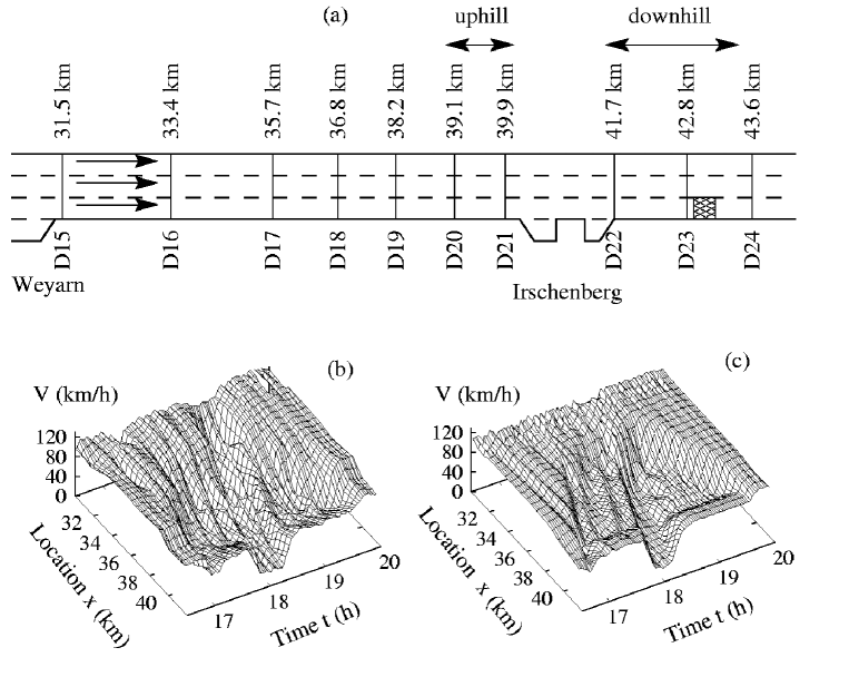
FIG. 1.: Traffic breakdown at a section of the A8-East used as test szenario. (a) Sketch of the section. The square downstream of D 23 indicates a temporary closing of the right lane due to an incident (see text). (b) Measured and (c) simulated locally averaged velocity.

III Traffic Control

Traffic controls influence the driving behavior of some or all vehicles. Some examples are

• speed limits,

• on-ramp controls (“ramp metering”),

• dynamic-route guidance systems, and

• lane-changing restrictions.

In addition to such externally imposed measures, a vehicle-based automated acceleration control is possible for vehicles equipped with driver-assistance systems.

Traffic control by ramp metering and route guidance is an old and large field ( for an overview, see, e.g., [9, 4]), while comparatively little has been published about modelling of speed limits [9, 10, 11, 12, 13]. In most cases, the effects of the above control measures on the static capacity have been investigated. We are not aware of a systematic simulation of the dynamic effects caused by various control measures using a single micromodel. We will show that dynamic effects are not only relevant but sometimes produce even counter-intuitive results. In particular, we will show that speed limits can increase the dynamic capacity although the average static capacity is even reduced.

In the following, we will simulate effects of a speed limit, an on-ramp control, and a driver-assistance system for a section of the German autobahn A8-East containing an uphill section around $x=40$ km. As further inhomogeneity, there is a small junction at about $x=41.0$ km. However, since the involved ramp flows were very small, we assumed that the junction had no dynamical effect.

We considered the situation during the evening rush hour on November 2, 1998. At about 17 h, traffic broke down at the uphill section. At about 18 h, an additional congestion caused by an incident further downstream propagated into the simulated section [7]. In the simulation shown in Fig. 1(c), we used measured lane-averaged one-minute data of velocity and flow as upstream and downstream boundary conditions. Both types of traffic breakdowns were realistically reproduced. For the purpose of simulating traffic controls, however, we will exclude the incident-caused jam, here, replacing the data-based downstream boundary conditions by “free” boundary conditions [14]. The reason is that congested traffic caused by accidents can be hardly eliminated by control measures. (The probability for an incident to occur can certainly be influenced, but this will not be discussed here).

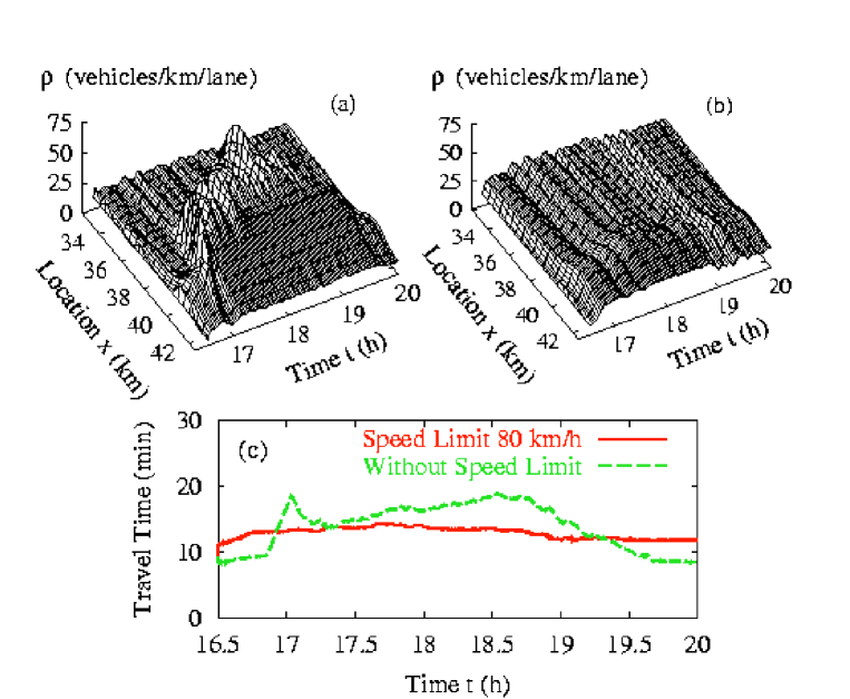
FIG. 2.: Simulation of the A8-East (a) without speed limit, (b) with a speed limit of 80 km/h. (c) Travel times corresponding to the scenarios (a) and (b).

A Speed limits

We have assumed two vehicle classes: 50% of the drivers had a desired velocity of $v_{0}=120$ km/h, while the other half had $v_{0}=160$ km/h outside of the uphill region. A speed limit reduces the desired velocities to 80 km/h. Within the uphill region, both driver-vehicle classes are forced to drive at a maximum of 60 km/h (for example, due to overtaking trucks that are not considered explicitely here; their realistic inclusion requires multi-lane simulations.)

Figure 2 shows spatio-temporal plots of the locally averaged traffic density for scenarios with and without the speed limit. (For the specific averaging formula, see Ref. [7].) The simulations show the following:

• During the rush hour (17 h $\leq t\leq 19$ h), the overall effect of the speed limit is positive. The increased travel times in regions without congestion are overcompensated by the saved time due to the avoided breakdown.

• For lighter traffic ($t<17$ h or $t>19$:30 h), however, the effect of the speed limit clearly is negative. This problem can be circumvented by traffic-dependent, variable speed limits.

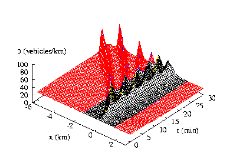
FIG. 3.: Simulation of an on-ramp with the micro-macro link (from [15]). The on-ramp region (dark) is computed with a macroscopic version of the IDM.

B On-Ramp Control

Traffic inflow on on-ramps can be controlled, e.g., by traffic lights (“ramp metering”). Many on-ramp flow-control strategies have been proposed in the last 30 years and applied mostly to macroscopic simulations [4]. Clearly, lane-changing processes play an important role in simulating on-ramp flow-control [9]. The role of the longitudinal dynamics (acceleration and braking), however, remained less clear.

Here, we will show that on-ramp control can be beneficial even when considering essentially longitudinal effects. To this purpose, we neglect lane changes on the main road and apply following minimal lane-changing scheme to implement an on-ramp of length $L_{\rm rmp}$ from which a traffic flow $Q_{\rm rmp}$ merges to a single main lane:

• Try to add ramp vehicles to the main flow at the times when the temporal ramp-flow integral reaches integer values.

• Search the largest gap on the main lane in the section of length $L_{\rm rmp}$ adjacent to the acceleration lane.

• If the resulting gaps to the respective front and rear vehicles exceed a certain minimal value, place the new vehicle in the middle with an initial velocity given by the average of the front and rear vehicles.

• Otherwise, add the vehicle to the queue of waiting vehicles. (This case did not occur in the simulations. All queues were caused by the flow control to be described below).

Another possibility (apart from a multi-lane model) is opened by the recently formulated micro-macro link [15] allowing to simulate the ramp section macroscopically with a source term in the continuity equation [16], while the remaining stretch is simulated microscopically, see Fig. 3.

We restrict the sum of the traffic flow $Q_{\rm main}$ upstream of the on-ramp and the flow $Q_{\rm rmp}$ arriving at the on-ramp by following simple control scheme:

$$Q^{\rm max}_{\rm rmp}=\max(0,Q_{\rm c}-Q_{\rm main}),$$ (3)

where $Q_{\rm main}$ is the traffic flow on the main road upstream of the on-ramp. If, at some time $t_{\rm c}$, the flow $Q_{\rm rmp}$ arriving at the on-ramp exceeds this limit, a queue of

$$n_{\rm wait}(t)=\int^{t}_{t_{c}}\!dt\,(Q_{\rm rmp}-Q^{\rm max}_{\rm rmp})$$ (4)

waiting vehicles will form. The actual inflow $Q^{c}_{\rm rmp}$ of the controlled on-ramp is given by

$$Q^{c}_{\rm rmp}=\left\{\begin{array}[]{ll}Q^{\rm max}_{\rm rmp}&\mbox{if }n_{\rm wait}(t)\geq 1,\\ \min(Q_{\rm rmp},Q^{\rm max}_{\rm rmp})&\mbox{otherwise.}\end{array}\right.$$ (5)

Notice that the on-ramp can be completely closed according to this scheme. More elaborate and realistic control schemes have been proposed in the literature [4]. The simulation results, however, are robust with respect to the choice of a certain control scheme, so we chose the conceivably most simple one.

We simulated single-lane single-class traffic and modelled the uphill gradient by reducing the desired velocity from 120 km/h to 60 km/h.

FIG. 4.: (a) Travel times on the main road (solid lines) and waiting times on the ramp (dashed) for $Q_{\rm rmp}=300$ vehicles/h. (b) Number of vehicles on the considered section of the main road and number of waiting on-ramp vehicles. All results are plotted for optimized flow control (thick lines), and without flow control (thin lines).

FIG. 5.: Travel and waiting times as in Fig. 4, but for non-optimal values of the cut-off flow $Q_{\rm c}$.

Figure 4 shows the travel time through the simulated section on the main road, and the waiting time at the on-ramp for an assumed ramp flow $Q_{\rm rmp}$ of 300 vehicles per hour and main lane for the optimal choice of $Q_{\rm c}$. Notice that in the optimized control scenario, the waiting times of the on-ramp vehicles are overcompensated by the decreased travel time for the main road stretch (with the exception of a short time interval after 17 h). Since also vehicles coming from the on-ramp drive on the main section afterwards, even they will generally profit from the flow control in this example.

Figure 5 shows the travel and waiting times for non-optimal values of $Q_{\rm c}$. If $Q_{\rm c}$ is 5% below the optimal value, the maximum waiting time is increased and becomes comparable to the saved travel time (Fig. 5 left). If one increases $Q_{\rm c}$ above the optimal value, the control becomes less and less effective (Fig. 5 right).

A suitable measure for assessing the quality of a traffic control is given by the sum of the waiting and travel times of all vehicles during the whole rush hour [4],

$$T_{\rm t}=\int^{t_{2}}_{t_{1}}\!dt\,[n_{\rm wait}(t)+n_{\rm main}(t)],$$ (6)

where $n_{\rm main}$ is the number of all vehicles in the considered section $x_{1}\leq x\leq x_{2}$. The spatio-temporal region $[t_{1},t_{2}]\times[x_{1},x_{2}]$ must be selected such that there is free traffic at all boundaries. Notice that the vehicle numbers and not the travel and waiting times enter into the quality measure $T_{\rm t}$. Furthermore, if $Q_{\rm main}(t)\leq Q_{\rm c}$ is satisfied for $t_{1}\leq x\leq t_{2}$, $T_{\rm t}$ does not depend on the on-ramp flow while the waiting times do. The right part of Fig. 4 illustrates the changes of the quality measure $T_{\rm t}$ induced by the control, see the difference between the areas enclosed by the two solid curves (saved total travel time for the main traffic) and by the dashed curve and the $x$-axis (total waiting time of the on-ramp traffic if the control is active).

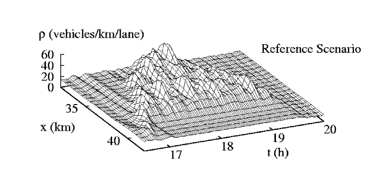
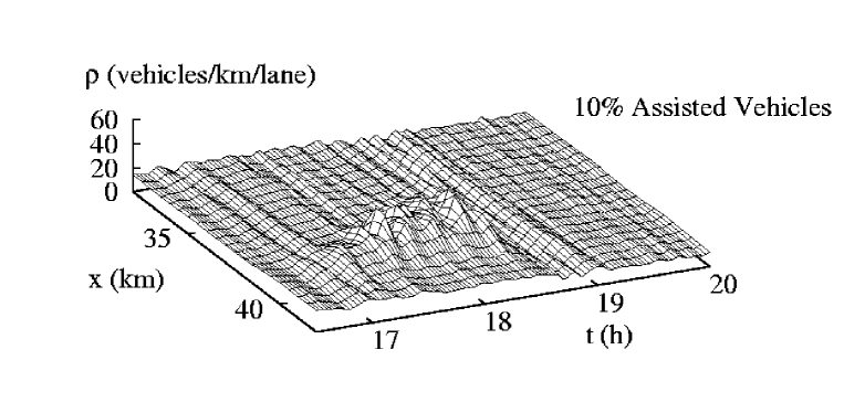
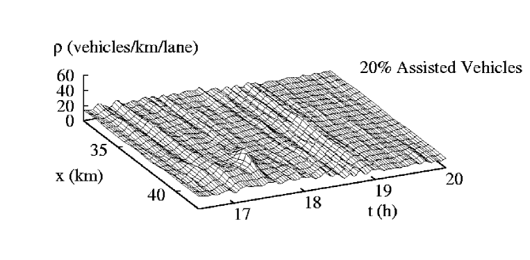
FIG. 6.: Spatio-temporal dynamics of the traffic density for different percentages of equipped vehicles. The acceleration of the equipped vehicles has been increased from $a=1$ m/s² to $a=2$ m/s². The time headway has been decreased from $T=1.6$ s to $T=0.8$ s.

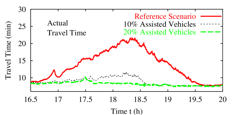
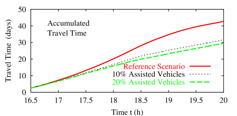
FIG. 7.: (a) Travel time of individual vehicles. (b) Total travel time of all vehicles for different percentages of equipped vehicles.

C Vehicle-Based Methods

The research presented in this section was performed in tight collaboration with the Volkswagen AG.

Presently, vehicle-based driver-assistance systems with adaptive acceleration control become available. In such systems, a detector determines the distance and velocity difference to the front vehicle and automatically accelerates or decelerates the vehicle according to the traffic situation. Obviously, micromodels like the IDM can be used to implement the control algorithm of such a system.

It may be argued that human and automated driving behaviours are fundamentally different. In fact, the assumptions of micromodels like the IDM: reaction only to the immediatel predecessor in combination with a negligible reaction time, fit perfectly to automated controls but less to human drivers. Human drivers have a non-negligible reaction time (of the order of 1 s) leading to more instability. This is offset by the more elaborate human driving strategy including direct reaction to decelerations (i.e., to braking lights) and anticipation of the traffic situations several vehicles in front of them. Nevertheless, the IDM can be calibrated to actual traffic data (cf. Fig. 1) suggesting that these two effects not contained in the IDM essentially cancel each other. This justifies the use of the same model for both human and automated longitudinal control.

Here, we show that, in principle, such control systems can improve the capacity and quality of traffic flow.

In the simulations, we model both equipped and not equipped vehicles with the IDM, using different values for $a$ and $T$. From the discussion of the IDM in Section II A one might expect that increasing $a$ for the equipped vehicles (within the range allowed by the motorization) increases stability of the overall traffic, while decreasing $T$ increases its capacity.

Figures 6 and 7 show that this is true even for only 10% equipped vehicles. The total additional time spent in the traffic jam was decreased by more than 80% with respect to the original situation. For a percentage of 20% equipped vehicles, the traffic breakdown disappeared almost completely.

IV Outlook and Discussion

In this paper, we have simulated the effects of speed limits, on-ramp controls, and driver-assistance systems using the microscopic intelligent-driver model (IDM). The IDM is suitable for simulating traffic controls because it is relatively simple, contains only a few and intuitive model parameters, and reproduces all relevant properties of real traffic. Moreover, it is numerically efficient and robust.

In all simulations, the model parameters have been calibrated to the historic traffic data of the respective reference scenarios. The presented effects of traffic control, however, are of a qualitative nature. They need to be calibrated before appying them in real control systems.

While our simulations of an on-ramp control support the findings obtained with macroscopic models [4, 9], we show that speed limits and driver-assistance systems have a similar beneficial potential. We emphasize that all three control measures have been simulated with the same model. Thus, it is possible to exploit the synergy effects that might result from a combination of these measures.

Both uphill gradients and speed limits reduce the velocity, so, at first sight, it is puzzling why speed limits can improve the quality of traffic flow while obviously uphill regions deteriorate it. To understand this, note that the desired velocity $v_{0}$ corresponds to the lowest value of

• the maximum velocity allowed by the motorization,

• the imposed speed limits, and (possibly with a “disobedience factor”),

• the velocity actually “desired” by the driver.

Therefore, speed limits act selectively on the faster vehicles, while uphill gradients reduce predominantly the desired velocity of the slower vehicles. As a consequence, speed limits reduce velocity differences, thereby stabilizing traffic, while uphill gradients increase them. Since global speed limits always raise the travel time in off-peak hours when free traffic is unconditionally stable, traffic-dependent speed limits are an optimal solution.

In contrast to speed limits, on-ramp controls are not common in Europe. We showed that, nevertheless, they can help to avoid or delay traffic breakdowns. Moreover, they can be advantageous even to the drivers who have to wait at the on-ramps because their total travel times are decreased as well.

The effects of on-ramp controls are qualitatively comparable to those of traffic-dependent, dynamic route guidance systems. While the former truncate flow peaks on a short time scale of the order of minutes, dynamic-route guidance systems truncate flow peaks on a time scale of hours.

In summary, our simulations support the conclusion that control measures which homogenize traffic flow are generally suitable for the reduction of congestion and travel times. While speed limits decrease speed differences, on-ramp controls smooth out flow peaks.

On the long run, however, vehicle-based systems have certainly the highest potential for increasing the traffic capacity of a given infrastructure. Driver-assistance systems can improve and speed up the reaction to the behavior of the respective vehicle in front. This allows stable traffic at significantly reduced time headways. In our test scenario, 20% equipped vehicles nearly eliminated all breakdowns. However, some legislatory and sensor-related problems remain to be solved.

Presently, we are extending our simulations to multi-lane traffic for the simulation of further control measures like lane-changing restrictions or overtaking bans for all or certain classes of vehicles (e.g., trucks). Moreover, we are exploring the potentials of communicating vehicles with respect to their optimal self-organization based on the paradigms of decentralized control and collective intelligence [17].

Acknowledgments: The authors are grateful for financial support by the DFG (grant no. He 2789/2-1). The research of Section III C was initiated and funded by the strategic research of the Volkswagen AG, Wolfsburg, and the results were produced in tight collaboration.

Parameter	Typical value
Desired velocity $v_{0}$	120 km/h
Safe time headway $T$	1.5 s
Maximum acceleration $a$	1 m/s2
Comfortable deceleration $b$	2 m/s2
Minimum distance $s_{0}$	2 m
Jam distance $s_{1}$	0 m
Acceleration exponent $\delta$	4

TABLE I.: Parameters of the IDM used as reference values.

REFERENCES

- [1] F. L. Hall and K. Agyemang-Duah, Freeway capacity drop and the definition of capacity, Transportation Research Record 1320, 91 (1991).
- [2] B. Persaud, S. Yagar, and R. Brownlee, Exploration of the breakdown phenomenon in freeway traffic, Transportation Research Record 1634, 64 (1998).
- [3] D. Helbing, Traffic and Related Self-Driven Many-Particle Systems, e-print http://arXiv.org/abs/cond-mat/0012229, to appear in Reviews of Modern Physics.
- [4] M. Papageorgiou, in Handbook of Transportation Science, edited by R. W. Hall (Kluwer Academic Publishers, London, 1999).
- [5] D. Chowdhury, L. Santen, and A. Schadschneider, Statistical physics of vehicular traffic and some related systems, Physics Reports 329, 199 (2000).
- [6] T. S. R. Wiedemann, Makroskopisches Simulationsmodel für Schnellstraßennetze mit Ber”ucksichtigung von Einzelfahrzeugen (DYNEMO), Straßenbau und Straßenverkehrstechnik, Heft 500 (Bundesministerium für Verkehr, Abt. Straßenbau, Bonn-Bad Godesberg, 1987).
- [7] M. Treiber, A. Hennecke, and D. Helbing, Congested Traffic States in Empirical Observations and Microscopic Simulations, Physical Review E 62, 1805 (2000).
- [8] M. Treiber, A. Hennecke, and D. Helbing, Microscopic Simulation of Congested Traffic, in Traffic and Granular Flow ’99, edited by D. Helbing, H. J. Herrmann, M. Schreckenberg, and D. E. Wolf (Springer, Berlin, 2000), pp. 365–376.
- [9] R. Lapierre and G. Steierwald, Verkehrsleittechnik für den Straßenverkehr, Band I: Grundlagen und Technologien der Verkehrsleittechnik (Springer, Berlin, 1987).
- [10] M. Cremer, Der Verkehrsfluß auf Schnellstraßen (Springer, Berlin, 1979).
- [11] S. Smulders, S., 1990, Control of freeway traffic flow by variable speed signs, Transpn. Res. B 24, 111 (1990).
- [12] R. D. Kühne, Freeway control using a dynamic traffic flow model and vehicle reidentification techniques, Transportation Research Record 1320, 251 (1991).
- [13] H. Lenz, Entwicklung nichtlinearer, diskreter Regler zum Abbau von Verkehrsflußinhomogenitäten mithilfe makroskopischer Verkehrsmodelle (Shaker Verlag, Aachen, 1999).
- [14] D. Helbing and M. Treiber, Numerical simulation of macroscopic traffic equations, Computing in Science and Engineering (CiSE) 5, 89 (1999).
- [15] A. Hennecke, M. Treiber, and D. Helbing, Macroscopic Simulations of Open Systems and Micro-Macro Link, in Traffic and Granular Flow ’99, edited by D. Helbing, H. J. Herrmann, M. Schreckenberg, and D. E. Wolf (Springer, Berlin, 2000), pp. 383–388.
- [16] D. Helbing and M. Treiber, Gas-Kinetic-Based Traffic Model Explaining Observed Hysteretic Phase Transition, Physical Review Letters 81, 3042 (1998).
- [17] D. Helbing and T. Vicsek, Optimal self-organization, New Journal of Physics 1, 13.1 (1999), see http://www.njp.org.