Phase transitions in a cluster molecular field approximation

Abstract

Cluster molecular field approximations represent a substantial progress over the simple Weiss theory where only one spin is considered in the molecular field resulting from all the other spins. In this work we discuss a systematic way of improving the molecular field approximation by inserting spin clusters of variable sizes into a homogeneously magnetised background. The density of states of these spin clusters is then computed exactly. We show that the true non-classical critical exponents can be extracted from spin clusters treated in such a manner. For this purpose a molecular field finite size scaling theory is discussed and effective critical exponents are analysed. Reliable values of critical quantities of various Ising and Potts models are extracted from very small system sizes.

. ]

I Introduction

The molecular field approximation (MFA) [1] is the method of choice to gain a first, usually qualitatively correct, understanding of phase diagrams in cases where exact results are not available. However, quantitative predictions derived in the framework of this approximation compare rather poorly with results obtained by other, more refined, methods. For example, the molecular field approximation systematically overestimates the temperatures at which phase transitions take place. This is of course due to the fact that correlations are completely neglected in this treatment. Furthermore, the critical exponents, describing the behaviour of critical quantities in the vicinity of a critical point, usually do not agree with the molecular field critical exponents. Above the upper critical dimension, however, the molecular field predictions of critical exponents become exact.

The shortcomings of the original MFA led Bethe [2] (see also Ref. [3] and [4]) to consider a more general treatment. In the Weiss theory of ferromagnetism, a single spin is considered in the molecular field which is caused by all the other spins. This is different in the Bethe approach where a small cluster of spins, consisting of the central spin and its nearest neighbours, is treated exactly. The molecular field acts exclusively on the edges of the cluster. Thus, correlations between a certain number of spins are included into the calculation. This is a significant improvement over simple molecular field theory, yielding for example critical temperatures which are much closer to the correct values than those obtained from the Weiss theory.

The general idea of inserting a cluster of spins into a homogeneously magnetised medium led to several applications in the past. Müller-Krumbhaar and Binder, for example, proposed a Monte Carlo method where a molecular field acts only on the surface spins of a cluster. This field has to be determined in a self-consistent way during the course of the simulation [5]. In a series of papers, Suzuki and coworkers established a general theoretical framework for extracting non-classical critical exponents from cluster-mean-field approximations [6, 7, 8, 9, 10, 11]. They considered a systematic series of clusters and showed that the true critical exponents can be obtained from the amplitudes of mean-field-type singularities. Various other generalisation schemes of the one-spin molecular field approximation have been discussed in the literature [12, 13].

In this work we present a systematic way of improving the molecular field approximation by considering spin clusters of variable sizes embedded into a homogeneously magnetised background. Hereby, the interactions within the clusters are taken into account exactly. To this end we compute the density of states as a function of the internal energy and of the interaction energy with a molecular field of unit strength. This is a hard task, but when it has been completed everything else does no longer demand time-consuming calculations. The actually applied molecular field itself is determined by imposing a condition of homogeneity in the central part of the cluster. This approach is used to evaluate various temperature dependent quantities for Ising models defined on different two- and three-dimensional lattices. A two-dimensional Ising model with nearest and next-nearest neighbour couplings has also been studied. Results obtained for three-state Potts models on square and triangular lattices are discussed, too.

With these data we demonstrate that critical quantities (critical temperatures as well as critical exponents) can be extracted reliably from the cluster molecular field approximation. This is already achieved by inserting very small clusters containing a small number of spins (the largest cluster studied is formed by 181 spins) into the molecular field. Besides analysing effective exponents we also show that the cluster molecular field data exhibit a remarkable finite size scaling behaviour which can be exploited for the determination of the true non-classical values of the critical exponents.

The paper is organised in the following way. In the next Section we present our method of systematically improving the molecular field approximation. We also discuss how to obtain various quantities from this data. In Section III the molecular field finite size scaling theory is discussed. We thereby use both the reduced temperature and the reduced energy as possible scaling variables. Section IV presents our data. We analyse them in different ways and show that critical quantities can be obtained from small clusters in a molecular field. Finally, in the last Section we present our conclusions.

II Clusters in a molecular field

In the following we propose a systematic scheme for improving the molecular field approximation. This scheme combines the exact computation of the density of states of small clusters with a molecular field acting solely on the borders of the clusters. In Section IV this method is applied to the determination of non-classical critical quantities of various Ising and three-state Potts models. Before discussing our approach in detail we will briefly reiterate the reasoning leading to the molecular field self consistency equation for these two models.

A The molecular field approximation

In zero field the Ising Hamiltonian reads

$$H_{I}=-J_{I}\sum_{\left<i,j\right>}\sigma_{i}\sigma_{j}$$ (1)

where $\sigma_{i}=\pm 1$ is an Ising spin on the lattice. Angular brackets denote sums over nearest neighbour pairs and $J_{I}$ is the exchange constant. The Hamiltonian for one selected spin $i$, given the spin values $\sigma_{i+\delta}$ of its $z$ neighbours, is

$$\tilde{H}_{I}=-J_{I}\,\sigma_{i}\sum_{\delta=1}^{z}\sigma_{i+\delta}.$$ (2)

If the spin $\sigma_{i}$ is considered and the rest of the lattice is replaced by a homogeneously magnetised medium with magnetisation $m$ then the spin variables $\sigma_{i+\delta}$ are replaced by the expectation value $\left<\sigma_{i+\delta}\right>=m$ and $\tilde{H}_{I}$ becomes $H_{I,MFA}(\sigma_{i})=-zJ_{I}\,m\,\sigma_{i}$ .

At the temperature T the expectation value of $\sigma_{i}$ in the molecular field $zJ_{I}\,m$ is:

$$\left<\sigma_{i}\right>=\frac{Z_{+}-Z_{-}}{Z}=\tanh(zJ_{I}m/k_{B}T)$$ (3)

where $Z_{+}=\exp(zJ_{I}m/k_{B}T)$ , $Z_{-}=\exp(-zJ_{I}m/k_{B}T)$ and $Z=Z_{+}+Z_{-}$ is the partition function for the two states of a single spin.

The condition $\left<\sigma_{i}\right>=m$ yields the self consistency equation which can be solved for the temperature

$$k_{B}T(m)/J_{I}=\frac{z\,m}{{\mbox{artanh}}(m)}\;.$$ (4)

Eq. (4) can be inverted or solved graphically if necessary. From the limit $m\to 0$ of (4) one finds the MFA critical temperature $k_{B}T_{c,MFA}/J_{I}=z$ and for small but finite $m$ one obtains

$$k_{B}T(m)/J_{I}=k_{B}T_{c,MFA}/J_{I}-\frac{z}{3}\>m^{1/\beta_{MFA}}+\ldots$$ (5)

with the critical exponent $\beta_{MFA}=1/2$.

The derivation of the corresponding self consistency equation for the three-state Potts model [14] defined by the Hamiltonian (the spins $\sigma_{i}$ taking the values 1, 2, 3)

$$H_{P}=-J_{P}\sum_{\left<i,j\right>}\delta(\sigma_{i},\sigma_{j})$$ (6)

with $\delta(\sigma_{i},\sigma_{j})=1$ if $\sigma_{i}=\sigma_{j}$ and zero otherwise is somehow more involved, so we only quote the result [15, 16]

$$m=\frac{\exp(zJ_{P}m/k_{B}T)-1}{\exp(zJ_{P}m/k_{B}T)+2}.$$ (7)

Inspection of the molecular field free energy reveals that at the temperature

$$k_{B}T_{c}/J_{P}=\frac{z}{4\ln(2)}$$ (8)

a first order transition takes place where the order parameter $m$ jumps from 0 to the value 1/2. This discontinuous behaviour in the MFA is in contrast to the fact that the temperature driven phase transition is continuous for the three-state Potts model in two dimensions.

These highly familiar results have been repeated also for the purpose of analysing the main defect of the approach. It is the lack of any correlation between the selected spin $\sigma_{i}$ and all the other spins in the lattice. This can be partially repaired if a cluster of $N$ spins is inserted into the homogeneously magnetised medium. In our approach, as discussed in the following, interactions within such clusters are taken into account exactly whereas the effect of the magnetised background is treated in the ordinary Weiss approximation. Therefore the correlations of the central spin with a number of neighbouring spins are included into the calculation thus leading to greatly improved results.

B Cluster molecular field approximation

In this Section we present our method to calculate physical quantities within an extended molecular field approximation based on the idea of Bethe.

Consider a classical spin system on a lattice defined by the Hamiltonian

$$H=\sum_{\left<i,j\right>}I(\sigma_{i},\sigma_{j})$$ (9)

where $I(\sigma_{i},\sigma_{j})$ is the interaction energy of the two neighbouring spins $\sigma_{i}$ and $\sigma_{j}$. For the Ising model this is just the negative product of the spin variables, i.e. $I_{I}(\sigma_{i},\sigma_{j})=-J_{I}\sigma_{i}\sigma_{j}$, for the $q$-state Potts model ($\sigma_{i}=1,\ldots,q$) the interaction energy is given by $I_{P}(\sigma_{i},\sigma_{j})=-J_{P}\delta(\sigma_{i},\sigma_{j})$. Suppose one has constructed a cluster of size $N$ by some method (see below) which is embedded in the original lattice. For this cluster the Hamiltonian (9) is replaced by the molecular field Hamiltonian

$$H_{N}=\sum_{\left<i,j\right>}I(\sigma_{i},\sigma_{j})+\mu\sum_{\{i,k\}}I(\sigma_{i},\sigma_{k})\delta(\sigma_{k},1)$$ (10)

where $\left<i,j\right>$ indicates a summation over nearest neighbour pairs within the cluster. The second term in (10) represents the interaction of the cluster with the homogeneously magnetised background. The sum runs over all pairs of nearest neighbour spins where the spin $\sigma_{i}$ is from inside the cluster and its partner $\sigma_{k}$ is from outside. This is denoted by the curly brackets. For convenience the $\sigma_{k}$ are set equal to 1 and their common expectation value $\left<\sigma_{k}\right>=\mu$ is placed outside the summation. The Hamiltonian (10) of the extended molecular field approximation treats the statistical mechanics of the spin system within the cluster exactly and the interaction of the cluster with the background is modelled by a molecular field that has to be determined in a self consistent way. In order to calculate physical quantities in the cluster molecular field approximation it is advantageous to work out the density of states

$$\Omega_{\sigma_{0},\sigma_{1}}(E,B)=\sum_{\Gamma_{N}(\sigma_{0},\sigma_{1})}\delta(H_{C},E)\delta(H_{B},B)\;,$$ (11)

with the internal energy of the cluster

$$H_{C}=\sum_{\left<i,j\right>}I(\sigma_{i},\sigma_{j})$$ (12)

and the interaction energy

$$H_{B}=\sum_{\{i,k\}}I(\sigma_{i},\sigma_{k})\delta(\sigma_{k},1)$$ (13)

of the cluster with the spins outside. The summation in (11) runs over all $\Gamma_{N}(\sigma_{0},\sigma_{1})$ states of the cluster with fixed spin value $\sigma_{0}$ of the central spin and $\sigma_{1}$ of one of its $z$ equivalent neighbours. For classical discrete spin models the density of states is just the number of configurations with specified values $E$, $B$, $\sigma_{0}$ and $\sigma_{1}$.

To work out physical quantities within this approximation scheme the density of states is evaluated exactly so that these quantities can be computed with arbitrary accuracy. The technical details of computing the density of states (11) for a given cluster size $N$ are summarised in the appendix. The size of the clusters which can be handled exactly is limited by the available computational capacities. To treat bigger clusters a recently proposed, highly efficient Monte Carlo algorithm to compute the density of states could be used [17]. However, a Monte Carlo calculation has to be performed with great care to achieve the desired accuracy.

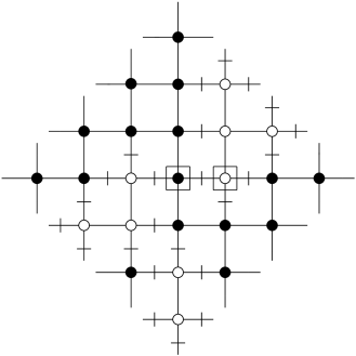
FIG. 1.: One of the $2^{25}$ configurations of an Ising cluster of 25 spins. Spin up $(\sigma_{i}=+1)$ is denoted by a full circle, spin down $(\sigma_{i}=-1)$ by an open circle. Broken bonds are marked with a little bar. Here $E=-6$ and $B=-10$. The central spin $\sigma_{0}=+1$ and one of its first neighbours $\sigma_{1}=-1$ are identified by little square. This configuration contributes one count to $\Omega_{+-}(-6,-10)=57642$.

Clusters of increasing particle numbers are selected in two different ways. A possible systematic series of clusters is constructed by choosing a spin to be the central spin and successively including shells of nearest neighbours. Hence, the first cluster of $z+1$ spins is made up of the central spin and its $z$ nearest neighbours. The next cluster consists of the first cluster and the shell of nearest neighbours of the border spins of the first cluster. By this way a new cluster is made up of the previous one together with the nearest neighbours of the boundary sites of the original cluster. This method has the advantage that assemblies of the same shape are build up. Fig. 1 displays the cluster of 25 spins emerging from this method for a two-dimensional square lattice. For the topology of the square lattice a cluster consists of $L$ rows of length $L$ perpendicular to the bisector of a quadrant of the plane and of $L-1$ short rows of length $L-1$ between the longer ones. Hence the number of spins in a cluster is given by $N=L^{2}+(L-1)^{2}$. The construction of successive clusters leads to a series of clusters with 5, 13, 25, 41, 61, 85, 113, 145, and 181 spins for the two-dimensional square lattice which can be handled with the available computational capacities. For the triangular lattice clusters of 7, 19, 37, 61, 91, and 127 spins emerge. In this geometry the basic row and the central row have the lengths $L$ and $2L-1$, respectively. However to avoid additional computational effort due to the length of the central row for the treatment of the triangular lattice we alternatively use the clusters of the square lattice by inserting additional bonds between the sites of the rows of lengths $L$ and $L-1$ so that all sites have the coordination number 6 of the triangular topology. In three dimensions the equivalent procedure would be restricted to only one, or at most two system sizes by the available storage capacities. This imposes a less systematic approach. The clusters are constructed by adding successive shells of neighbours of the central spin. With the nearest neighbours of the central spin one obtains a cluster of 7 spins, with the next nearest neighbours the size is 19, then 27, 33, 57, and so on. The cluster of 57 spins that consists of the central spin and includes all spins up to the 5th neighbours was the largest one which could be handled in three dimensions. This way of selecting clusters for the three-dimensional case has the disadvantage that the various assemblies do not have the same geometry.

Once the density of states is known physical quantities are easily evaluated. For example the expectation value of the central spin is given by

$$\left<\sigma_{0}\right>=\sum_{\sigma_{0},\sigma_{1}}\sigma_{0}Z_{\sigma_{0},\sigma_{1}}/Z$$ (14)

with the restricted partition functions

$$Z_{\sigma_{0},\sigma_{1}}=\sum_{E,B}\Omega_{\sigma_{0},\sigma_{1}}(E,B)\exp\left(-(E+\mu B)/k_{B}T\right)$$ (15)

and the total partition function

$$Z=\sum_{\sigma_{0},\sigma_{1}}Z_{\sigma_{0},\sigma_{1}}\;.$$ (16)

Similarly the expectation value of the spin $\sigma_{1}$ is computed from (11). The unknown homogeneous magnetisation $\mu$ of the sites outside the cluster must be determined self consistently. When the expectation value $\left<\sigma_{0}\right>$ of the central spin is calculated as a function of $\mu$ and $T$ the temperature might be adjusted such that $\left<\sigma_{0}\right>$ is equal to $\mu$:

$$\left<\sigma_{0}\right>(T)=\mu(T)\;.$$ (17)

Thereby the rigid external magnetisation is moved further away from the central spin and an improvement of the plain molecular field approximation is observed [10]. This is the usual condition to determine the molecular field discussed in the literature. Nevertheless only the central spin is directly related to the rigid background magnetisation through the self-consistency equation so that the expectation values of the central spin and one of its neighbour spins are different. In our approach the condition

$$\left<\sigma_{0}\right>(T)=\left<\sigma_{1}\right>(T)$$ (18)

is used instead. This condition, which implicitly determines $\mu$ as a function of $T$, ensures that the spin in the centre of the cluster and its neighbouring spins have the same expectation value so that at least in the central part of the cluster the equivalence of the spins is implemented. The spins in the centre of the cluster are not directly coupled to the rigid background magnetisation. In the extended molecular field approximation based on condition (18), fluctuations of the expectation value of a spin near the border of the cluster are suppressed due to the direct coupling to the homogeneous background magnetisation whereas the central spin can develop comparatively large fluctuations. The behaviour of the central spin in the approximation used is consequently most closely related to the corresponding behaviour of a spin in the infinite system. The same holds for the interaction energies of bonds in the centre compared to those of bonds near the boundary of the cluster. These aspects suggest that the calculation of physical quantities should be restricted to the central part of the cluster where the condition of homogeneity is rather well fulfilled.

FIG. 2.: Order parameters as function of temperature (full lines) as obtained from the cluster molecular field approximation for various two-dimensional Ising models defined on a square lattice. System sizes from right to left: 13, 25, 41, 61, 85, 114 145, and 181 spins. The spontaneous magnetisation of the infinite system is shown as a dashed line. For systems treated in the cluster molecular field approximation the order parameter sets in abruptly at a pseudo-critical temperature, see Table I. At low temperatures the finite size order parameters follow closely the spontaneous magnetisation of the infinite system.

After solving the implicit equation (18) for the molecular field all physical quantities can be evaluated using the density of states (11). The order parameter of the system is determined from $\left<\sigma_{0}\right>$. Note that in the limit $T\to 0$ the interaction of the border spins of the cluster with the homogeneously magnetised background forces all spin variables to be in the spin state $\sigma=1$ of the spins outside the cluster. For the Ising model the order parameter is given by

$$m_{I}(T)=\left<\sigma_{0}\right>(T)$$ (19)

and for the $q$-state Potts model one has

$$m_{P}(T)=\frac{q\left<\sigma_{0}\right>(T)-1}{q-1}\;.$$ (20)

In the cluster molecular field approach the order parameter is exactly zero at high temperatures. When decreasing the temperature the order parameter of the Ising model exhibits a sudden onset at the temperature $T_{c,N}$ indicating a transition to a magnetised phase. The abrupt appearance of a finite order parameter defines the pseudo-critical temperature of the finite system. Fig. 2 illustrates this temperature dependent behaviour of the order parameter in the case of the square lattice Ising model. It is instructive to compare the pseudo-critical temperatures resulting from equations (17) and (18). For a cluster of $N=145$ spins defined on the square lattice our approach (18) leads to the value $k_{B}T_{c,N}/J_{I}=2.37096$ ($T_{c,N}/T_{c}=1.045$, where $k_{B}T_{c}/J_{I}=2/\ln(1+\sqrt{2})$ is the critical temperature of the two-dimensional Ising model defined on the square lattice), which should be compared to the value 2.57524 ($T_{c,N}/T_{c}=1.135$) obtained when using the self-consistency equation (17) [10]. A similar remarkable improvement is also achieved for three-dimensional clusters: for $N=57$ spins our pseudo-critical temperature is $k_{B}T_{c,N}/J_{I}=4.6627$ ($T_{c,N}/T_{c}=1.034$), much closer to the value $4.5115$ of the infinite system than the value $5.0018$ ($T_{c,N}/T_{c}=1.109$) resulting from Eq. (17) [10]. The pseudo-critical temperatures of the Ising model for various lattice topologies are summarised in Table I and Table II for the two-dimensional and the three-dimensional systems, respectively.

In Fig. 3 we show the order parameter for the three-state Potts model defined on a square lattice as a function of temperature for a series of cluster sizes. For all clusters a jump in the order parameter is observed, thus disclosing the discontinuous character of the phase transition in the MFA. This jump gets smaller when the number of cluster spins is increased reflecting the softening of the first order character of the phase transition with increasing cluster size. In the limit $N\longrightarrow\infty$ the jump will disappear completely in accordance with the continuous phase transition taking place in the bulk three-state Potts model. The temperature at which the jump occurs is deduced from the behaviour of the free energy. The values of these transition temperatures are displayed in Table III for the square and the triangular lattice.

We estimate the internal energy from the bonds of the central spin with its $z$ neighbour spins which yields

$$u(T)=\frac{z}{2}\sum_{\sigma_{0},\sigma_{1}}I(\sigma_{0},\sigma_{1})Z_{\sigma_{0},\sigma_{1}}/Z\;.$$ (21)

TABLE I.: The pseudo-critical temperatures $T_{c,N}$ of the two-dimensional Ising model defined on the square (sq) and the triangular (tr) lattice.

$N$	sq	tr
$\infty$	$2.26919$	$3.64096$
$181$	$2.36008$	$\ldots$
$145$	$2.37096$	$3.82574$
$113$	$2.38480$	$3.85042$
$85$	$2.40294$	$3.88338$
$61$	$2.42778$	$3.92602$
$41$	$2.46380$	$3.99458$
$25$	$2.52078$	$4.0804$
$13$	$2.62534$	$4.27958$
$5$	$2.88539$	$4.72088$

TABLE II.: The pseudo-critical temperatures $T_{c,N}$ of the three-dimensional Ising model on the simple cubic (sc) lattice.

$N$	sc
$\infty$	$4.5115$
$57$	$4.66266$
$33$	$4.69361$
$27$	$4.69367$
$19$	$4.74872$
$7$	$4.93261$

TABLE III.: The transition temperatures of the three-state Potts models defined on the square (sq) and the triangular (tr) lattice.

$N$	sq	tr
$\infty$	$0.99497$	$1.58493$
$85$	$1.01937$	$1.62849$
$61$	$1.02396$	$1.63619$
$41$	$1.03051$	$1.64813$
$25$	$1.04074$	$1.66267$
$13$	$1.05957$	$1.69818$

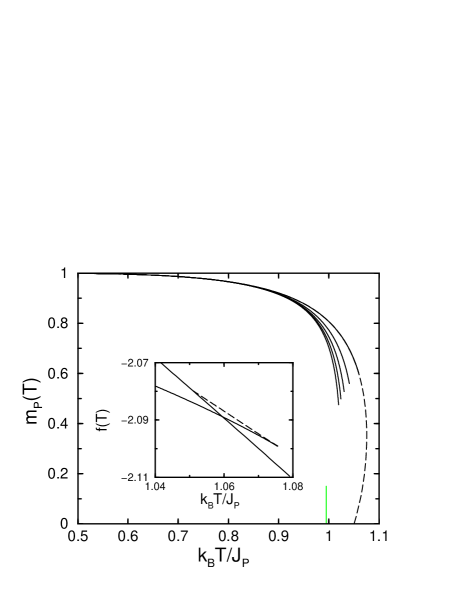
FIG. 3.: Temperature dependent order parameters of three-state square lattice Potts models derived within the cluster molecular field approximation (full lines). The exactly treated clusters contain (from right to left) 13, 25, 41, 61, and 85 spins. The discontinuous character of the phase transition in the cluster molecular field approximation is displayed by the jump of the order parameter. The unstable solution for a system with 13 spins is shown as a dashed line. The grey line indicates the location of the critical point of the infinite system: $k_{B}T_{c}/J_{P}=1/\ln(\sqrt{3}+1)\approx 0.995$. Inset: free energies obtained for a cluster with 13 spins within the cluster molecular field approximation. The free energy of the stable high and low temperature phases are shown as full lines whereas the dashed line is the free energy of the unstable solution. The intersection of the full lines yields the transition temperature listed in Table III.

From the internal energy one now gets the specific heat

$$c(T)=\frac{du(T)}{dT}\;.$$ (22)

The specific heat is also related to the entropy of the central spin through the relation

$$c(T)=T\frac{ds(T)}{dT}\;.$$ (23)

This allows the computation of the free energy

$$f(T)=u(T)-Ts(T)$$ (24)

from the knowledge of the internal energy. Solving equation (23) for the entropy $s(T)$ one obtains the free energy

$$f(T)=u(T)-T\int_{T_{0}}^{T}d\tau\frac{c(\tau)}{\tau}$$ (25)

with $T_{0}$ being some arbitrarily chosen temperature representing the constant of integration. The free energy of the Potts model for the cluster with 13 spins in the vicinity of the transition point is shown in the inset of Fig. 3. The solution of (20) that minimises the free energy is physically stable. This leads to the kink of the free energy at the transition temperature again indicating the discontinuity of the phase transition for finite $N$.

Next we consider the response of the central spin to an external field that acts exclusively on the central spin itself. In order to evaluate this zero field susceptibility one has to differentiate the magnetisation with respect to a magnetic field that acts only on the central spin variable $\sigma_{0}$:

$$\chi(T)=\lim_{h\to 0}\frac{\partial m(T,h)}{\partial h}\;.$$ (26)

To obtain an analytic expression for the susceptibility of the Ising model we add a magnetic field term to the Hamiltonian:

$$H_{I}\rightarrow H_{I}-h\sigma_{0}\;.$$ (27)

When evaluating the susceptibility one has to bear in mind that one gets a field-dependent molecular field $\mu=\mu(T,h)$ due to this additional external field $h$. This has the consequence that (26) depends on the derivative of $\mu$ with respect to the magnetic field $h$. However, the order parameter $m$ is given by the two equivalent equations $m=\left<\sigma_{0}\right>$ and $m=\left<\sigma_{1}\right>$ so that one of them can be used to eliminate $\partial\mu/\partial h$ from (26). Differentiating $\left<\sigma_{0}\right>$ with respect to $h$ one obtains the expression

$$\chi(T,h)=\frac{1}{k_{B}T}\left[\left<\sigma_{0}^{2}\right>-\left<\sigma_{0}\right>^{2}+\frac{\partial\mu}{\partial h}(\left<\sigma_{0}\right>\left<B\right>-\left<\sigma_{0}B\right>)\right]\;.$$ (28)

On the other hand differentiation of $\left<\sigma_{1}\right>$ yields

$$\chi(T,h)=\frac{1}{k_{B}T}\left[\left<\sigma_{0}\sigma_{1}\right>-\left<\sigma_{0}\right>^{2}+\frac{\partial\mu}{\partial h}(\left<\sigma_{0}\right>\left<B\right>-\left<\sigma_{1}B\right>)\right]\;.$$ (29)

Combining these two relations in order to eliminate the derivative of the molecular field results in the desired expression of the zero-field susceptibility for temperatures below $T_{c,N}$:

$$\chi(T) = \frac{1}{k_{B}T}\left[\left<\sigma_{0}^{2}\right>-\left<\sigma_{0}\right>^{2}\right.$$ (31)

$$-\left.\frac{(\left<\sigma_{0}\right>\left<B\right>-\left<\sigma_{0}B\right>)(\left<\sigma_{0}^{2}\right>-\left<\sigma_{0}\sigma_{1}\right>)}{\left<\sigma_{0}B\right>-\left<\sigma_{1}B\right>}\right]\;.$$

The first two terms in the square brackets represent the ordinary fluctuation formula for the susceptibility. The additional third term arises from the coupling to the molecular field. Its denominator vanishes in the limit $T\to T_{c,N}$ yielding a diverging susceptibility for $T\to T_{c,N}$ as expected for the molecular field approach. Fig. 4 displays the zero field susceptibility of the two-dimensional Ising model defined on the square lattice for different cluster sizes.

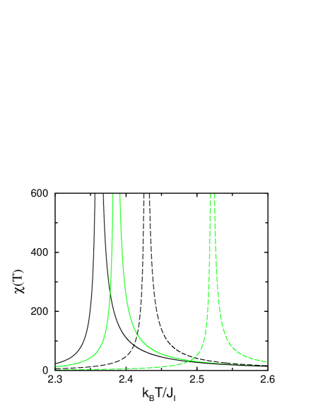
FIG. 4.: Zero field susceptibilities as function of temperature obtained from the cluster molecular field treatment of two-dimensional square lattice Ising clusters, see Eq. (31). The susceptibilities diverge at the pseudo-critical temperatures. The Ising clusters contain 25, 61, 113, and 181 spins.

For the $q$-state Potts model the magnetic field acts on the central spin only if it is in the spin state $\sigma$ of the sites outside the cluster:

$$H_{P}\rightarrow H_{P}-h\delta(\sigma_{0},\sigma)\;.$$ (32)

The susceptibility of the Potts model for temperatures below the pseudo-critical point of the finite cluster is then given by

$$\chi(T) = \frac{q}{q-1}\frac{1}{k_{B}T}\left[\left<\sigma_{0}\delta(\sigma_{0},\sigma)\right>-\left<\sigma_{0}\right>\left<\delta(\sigma_{0},\sigma)\right>\right.$$ (34)

$$-\left.\frac{(\left<\sigma_{0}\right>\left<B\right>-\left<\sigma_{0}B\right>)(\left<\sigma_{0}\delta(\sigma_{0},\sigma)\right>-\left<\sigma_{1}\delta(\sigma_{0},\sigma)\right>)}{\left<\sigma_{0}B\right>-\left<\sigma_{1}B\right>}\right]\;.$$

This expression for the Potts model has the same structure as the corresponding expression (31) of the Ising model. However the susceptibility of the Potts model does not diverge as the molecular field displays a jump at the transition temperature.

III Molecular field finite size scaling theory

In this Section we present a phenomenological finite size scaling theory for our cluster molecular field approximation. We consider both the reduced temperature and the reduced energy as scaling variables and discuss the relative size of the corrections to scaling. Our data are then analysed in the following Section using the framework of the molecular field finite size scaling to be exposed in the following subsection.

A Finite size scaling for the temperature picture

The spontaneous magnetisation of the cluster molecular field approximation displays the characteristics of spontaneous symmetry breaking. This allows an unambiguous definition of the pseudo-critical temperature $T_{c,L}$ of the finite system of linear extension $L$ taken to be $N^{1/d}$ where $d$ is the dimensionality of the lattice. The spontaneous magnetisation near this pseudo-critical temperature then behaves like

$$m_{sp,L}(t^{\prime})=A_{L}(-t^{\prime})^{\beta^{\prime}}$$ (35)

where the reduced temperature $t^{\prime}$ is defined as

$$t^{\prime}=\frac{T-T_{c,L}}{T_{c,L}}$$ (36)

and where $\beta^{\prime}=0.5$ is the molecular field critical exponent. For increasing clusters the influence of the molecular field which acts only on the boundary becomes weaker so that the approximation eventually becomes exact in the limit $L\to\infty$. In the infinite system the spontaneous magnetisation vanishes like

$$m_{sp}(t)=A(-t)^{\beta}$$ (37)

for small reduced temperatures $t$ which is related to the critical temperature $T_{c}=T_{c,\infty}$ of the infinite system by

$$t=\frac{T-T_{c}}{T_{c}}\;.$$ (38)

The fractional shift $\tau_{L}$ is given by [18]

$$\tau_{L}=\frac{T_{c}-T_{c,L}}{T_{c}}\sim-DL^{-\lambda}$$ (39)

with the shift exponent $\lambda=1/\nu$ where $\nu$ is the critical exponent of the correlation length. Equation (39) and (36) are combined to yield

$$t^{\prime}=t+\tau_{L}+O(\tau^{2}_{L})$$ (40)

for large $L$. Equation (39) can be used to obtain an approximation of the transition temperature in the thermodynamic limit. This is exploited in Section IV.

For sufficiently small $t^{\prime}$ we assume that the spontaneous magnetisation of the finite system of extension $L$ is given by

$$m_{sp,L}(t^{\prime})=L^{p}\phi(t^{\prime}L^{1/\nu})\;.$$ (41)

The function $\phi(x)$ is universal showing no further $L$-dependence. The exponent $p$ in (41) is obtained by taking the limit $L\to\infty$ for fixed temperature $T\neq T_{c}$. In this limit equation (41) reduces to (37) yielding

$$\phi(x)\sim x^{\beta}\mbox{ as }x\to\infty\;.$$ (42)

The residual $L$ dependence is cancelled out if $p=-\beta/\nu$. Hence the finite size scaling relation

$$L^{\beta/\nu}m_{sp,L}(t^{\prime})=\phi(t^{\prime}L^{1/\nu})$$ (43)

follows.

At this point we have to mention that an unambiguous definition of the linear extension of our finite clusters is not possible. This crucial fact was already pointed out in [7]. For our investigations we choose $L=N^{1/d}$ but other definitions are also possible. For the three-dimensional systems our choice is especially problematic as the clusters do not have the same geometry. We will come back to this point in Section IV when discussing our numerical data.

From equation (35) follows that the universal function $\phi$ behaves like a square root for small scaling variables, i.e.

$$\phi(t^{\prime}L^{1/\nu})=A_{\phi}\sqrt{-t^{\prime}L^{1/\nu}}\;,$$ (44)

for $t^{\prime}\to 0$ and fixed $L$. Taking the limit $t^{\prime}\to 0$ and comparing with relation (41) the finite size scaling law

$$A_{L}=A_{\phi}L^{\frac{\beta^{\prime}-\beta}{\nu}}$$ (45)

for the amplitudes of the magnetisation of the finite systems is derived.

In an analogous way we obtain a finite size scaling relation for the susceptibility. In the molecular field approach the susceptibility diverges with the molecular field critical exponent $\gamma^{\prime}=1$. We then have the scaling relation

$$L^{-\gamma/\nu}\chi_{L}(t^{\prime})=\psi(t^{\prime}L^{1/\nu})\;,$$ (46)

where for small scaling variables the universal function $\psi$ is given by

$$\psi(t^{\prime}L^{1/\nu})=A_{\psi}\,(t^{\prime}L^{1/\nu})^{-1}\;.$$ (47)

One also derives, in complete analogy with Eq. (45), a finite size scaling law involving the finite size amplitudes of the susceptibility. Note that this relation was already used in references [7, 10] to get estimates for the critical exponent $\gamma$. All these relations show that the critical exponents of the infinite system are encoded in the amplitudes of the corresponding quantity of the finite system. It is precisely this fact which will allow the determination of critical exponents from the cluster molecular field approximation. It is also worth noting that in the present approach the critical temperature of the infinite system is not needed for the determination of critical exponents.

B Finite size scaling for the energy picture

The internal energy of a system is given by the expectation value (21). The expression $u_{L}=u_{L}(T)$ can be inverted in order to obtain the temperature as a function of the internal energy of the system. All physical quantities can then be expressed as functions of the internal energy. In the following subsections this transformation from the temperature picture to the energy picture is discussed for systems displaying either an algebraically or a logarithmically diverging specific heat in the thermodynamic limit.

1 Algebraically diverging specific heat

Consider the spontaneous magnetisation near the pseudo-critical point of the finite system:

$$m_{sp,L}(t^{\prime})=A_{\phi}L^{\frac{\beta^{\prime}-\beta}{\nu}}\sqrt{-t^{\prime}}(1+B_{L}t^{\prime}+\ldots)$$ (48)

where a correction term to the leading behaviour with the $L$-dependent amplitude $B_{L}$ is explicitly taken into account. From finite size scaling theory one obtains a similar expression for the (intensive) zero-field specific heat near $t^{\prime}=0$ for negative $t^{\prime}$:

$$c_{h=0,L}(t^{\prime})=aL^{\frac{\alpha-\alpha^{\prime}}{\nu}}(1+2b_{L}t^{\prime}+\ldots)$$ (49)

with an $L$-dependent amplitude of the linear correction term. Here it is assumed that the singularity of the specific heat of the infinite system is characterised by $\alpha\neq 0$. The case of a logarithmic divergence is deferred to the next subsection. Note also that the specific heat in molecular field approximation does not diverge. It exhibits a jump singularity, hence one has the exponent $\alpha^{\prime}=0$. At the pseudo-critical point of the finite system, i.e. $t^{\prime}=0$, equation (49) reduces to

$$C_{L}=c_{h=0,L}(0)=aL^{\frac{\alpha-\alpha^{\prime}}{\nu}}\;.$$ (50)

This relation can be used to estimate the true critical exponent $\alpha$ from the maxima of the specific heat of the various finite systems.

As

$$c_{h=0,L}=\frac{du(T)}{dT}=\frac{du}{dt^{\prime}}\frac{dt^{\prime}}{dT}=\frac{1}{T_{c,L}}\frac{du}{dt^{\prime}}$$ (51)

integration of (49) gives

$$\varepsilon^{\prime}(t^{\prime})=u_{L}(t^{\prime})-u_{c,L}$$ (52)

with $u_{c,L}$ being the constant of integration. This constant is just the pseudo-critical energy of the finite system. The expression for $\varepsilon^{\prime}(t^{\prime})$ can be inverted for small $t^{\prime}$ to give

$$t^{\prime}=\frac{1}{T_{c,L}a}L^{-\alpha/\nu}\varepsilon^{\prime}-\frac{b_{L}}{T_{c,L}^{2}a^{2}}L^{-2\alpha/\nu}\varepsilon^{\prime 2}+\ldots$$ (53)

in the asymptotic limit $\varepsilon^{\prime}\to 0$. Plugging this result in equation (48) one finally obtains

$$m_{sp,L}(\varepsilon^{\prime}) = A_{\phi}L^{\frac{\beta^{\prime}-\beta_{\varepsilon}}{\nu_{\varepsilon}}}\sqrt{\frac{-\varepsilon^{\prime}}{aT_{c,L}}}$$ (55)

$$\left(1+L^{-\alpha/\nu}\frac{1}{aT_{c,L}}(B_{L}-b_{L})\varepsilon^{\prime}+\ldots\right)$$

with the renormalised exponents $\beta_{\varepsilon}=\frac{\beta}{1-\alpha}$ and $\nu_{\varepsilon}=\frac{\nu}{1-\alpha}$. These renormalised critical exponents describe the singular behaviour of the various thermostatic quantities of the infinite system in the energy picture [19]. The reformulation also yields the finite size scaling relation

$$L^{\beta_{\varepsilon}/\nu_{\varepsilon}}m_{sp,L}(\varepsilon^{\prime})=\tilde{\phi}\left(\frac{\varepsilon^{\prime}L^{1/\nu_{\varepsilon}}}{T_{c,L}}\right)$$ (56)

for the energy picture with a scaling variable that contains the transition temperature of the finite system. In a completely analogous way the reformulation can be done for other physical quantities like the susceptibility. For large systems the pseudo-critical temperature $T_{c,L}$ is close to the critical temperature of the infinite system so that is can be replaced by $T_{c}$. However, as we are dealing with very small clusters the additional $L$-dependence in the scaling variable due to $T_{c,L}$ can not be neglected. Similar to equation (39) one obtains the shift relation for the pseudo-critical energy:

$$e_{L}=\varepsilon_{c,\infty}-\varepsilon_{c,L}\sim-D_{\varepsilon}L^{-1/\nu_{\varepsilon}}\;.$$ (57)

The proposed scaling variable for the energy picture and the corresponding scaling relations are tested in Section IV.

In equation (55) the amplitude of the linear correction term contains the amplitudes $B_{L}$ and $b_{L}$ of the temperature picture. Moreover a prefactor $L^{-\alpha/\nu}$ appears which will lead to a suppression of the leading correction term compared to the corresponding expression (48) in the temperature picture if the critical exponent $\alpha$ is positive. This suppression is determined by the prefactor together with the $L$-dependence of the amplitudes $B_{L}$ and $b_{L}$. If the amplitudes grow strongly enough with the system size the suppression becomes weaker for increasing $L$. Note however that a reduction of the linear corrections in the energy picture will eventually always take place even if this reduction becomes weaker for larger cluster sizes. For a system with a negative exponent the correction term in the energy picture is blown up relative to the temperature picture. The investigation of this interesting consequence in the $3d$ Heisenberg model as an example of a system with $\alpha<0$ is left to future studies.

2 Logarithmically diverging specific heat

With slight modifications the above discussed transfer to the energy picture is carried out for the case of a logarithmically diverging specific heat $c=-A\ln t$ of the infinite system. A prominent example of such a system is the two-dimensional Ising model. In this case the amplitude $C_{L}$ (i.e. the maximum) of the finite system specific heat varies as [20]

$$C_{L}=A\ln L^{1/\nu}+\xi=A^{\prime}\ln L+\xi\;.$$ (58)

FIG. 5.: Specific heat maxima as function of $\ln L$ for small two-dimensional Ising clusters defined on a square lattice. The linear extension $L$ is given by $L=\sqrt{N}$ where $N$ is the total number of spins forming the cluster. The dashed line results from fitting these data to Eq. (58), with $A^{\prime}=0.562$ and $\xi=1.76$.

Fig. 5 shows equation (58) for the $2d$ Ising model in the extended molecular field approximation. The depicted linear behaviour is characterised by the slope $A^{\prime}=0.562$ and the intercept $\xi=1.76$ with the vertical axis. For sufficiently large system sizes the $L$-independent constant $\xi$ can be neglected relative to the increasing contribution from the logarithmic term. As relatively small systems are considered in the molecular field approximation discussed here this constant is explicitly taken into consideration. The arguments used to replace the variable $t^{\prime}$ by the internal energy still apply and give rise to the relation

$$m_{sp,L}(\varepsilon^{\prime}) = A_{\phi}L^{\frac{\beta^{\prime}-\beta_{\varepsilon}}{\nu_{\varepsilon}}}\sqrt{\frac{-\varepsilon^{\prime}}{(A^{\prime}\ln L+\xi)T_{c,L}}}$$ (60)

$$\left(1+\frac{1}{(A^{\prime}\ln L+\xi)T_{c,L}}(B_{L}-b_{L})\varepsilon^{\prime}+\ldots\right)\;.$$

The linear correction term is again diminished by an additional $L$-dependent prefactor as already observed for systems with $\alpha>0$. This form of the magnetisation suggests the finite size scaling law

$$L^{\beta_{\varepsilon}/\nu_{\varepsilon}}m_{sp,L}(\varepsilon^{\prime})=\tilde{\phi}\left(\frac{\varepsilon^{\prime}L^{1/\nu_{\varepsilon}}}{(A^{\prime}\ln L+\xi)T_{c,L}}\right)=\tilde{\phi}\left(\frac{\varepsilon^{\prime}L^{1/\nu_{\varepsilon}}}{C_{L}T_{c,L}}\right)$$ (61)

with a slightly modified scaling variable. This modified scaling variable in the energy picture is investigated for the two-dimensional Ising model in the next Section. Note however that the factor causing the suppression of the linear correction term of the magnetisation is now integrated into the scaling variable. This has the consequence that the reduction of the corrections to scaling in (61) are solely controlled by the relative size of the amplitudes $B_{L}$ and $b_{L}$. Therefore it has to be expected that the reduction of the corrections are weaker than those in the case of an algebraically diverging specific heat.

IV Critical quantities

In this Section we extract critical quantities like critical exponents or transition temperatures of the infinite system from the molecular field data of the corresponding finite systems. Apart from the molecular field finite size scaling relations presented in the previous Section the notion of the effective critical exponent provides another way to obtain critical exponents from finite system quantities [21].

The effective critical exponent $\beta_{eff,N}$ of the order parameter is defined by expressing the temperature dependent spontaneous magnetisation $m_{N}$ in the form

$$m_{N}=A\,t^{\beta_{eff,N}(T)}\;,$$ (62)

where $t=(T_{c}-T)/T_{c}$ and $T_{c}$ is again the critical temperature of the infinite system. The temperature dependent effective exponent is obtained by differentiating relation (62):

$$\beta_{eff,N}(T)=\frac{d\ln(m_{N})}{d\ln t}\;.$$ (63)

Fig. 6 shows the effective exponent of the two-dimensional Ising model for the different clusters on the square lattice together with the effective critical exponent $\beta_{eff,\infty}$ of the infinite system [22]. As the pseudo-critical temperatures of the finite systems are above the critical temperature $T_{c}$ of the infinite system the spontaneous magnetisation $m_{N}(T)$ is finite at $T_{c}$ and therefore the effective exponent has to vanish at $T_{c}$. It is also observed that the effective exponents of the largest clusters are closer to the corresponding curve of the infinite system than those of the small clusters. From the effective exponents estimates for the true critical exponent $\beta$ may be extracted by means of linear extrapolation. To this end an extrapolated exponent $\beta_{ext,N}$ is defined by

$$\beta_{ext,N}(T)=\beta_{eff,N}(T)+\frac{d\beta_{eff,N}(T)}{dT}(T_{c}-T)\;.$$ (64)

This extrapolated exponent is displayed in Fig. 7 for the square lattice again together with $\beta_{ext,\infty}$ of the infinite system. Note that the effective exponent depends on the critical temperature of the infinite lattice. For models with an unknown value of $T_{c}$ a reliable estimate has to be obtained from the finite system pseudo-critical temperatures. This can be achieved by using the finite size scaling relation (39).

FIG. 6.: Effective critical exponents $\beta_{eff,N}$ versus temperature for different square lattice Ising clusters. The system sizes are the same as those in Fig. 2, the lowest line resulting from the cluster with 13 spins. These curves directly follow from the logarithmic derivative of the spontaneous magnetisations displayed in Fig. 2 with respect to the temperature. The dashed line is the effective critical exponent of the infinite system, yielding the critical exponent $\beta=1/8$ in the limit $T\longrightarrow T_{c}$.

FIG. 7.: Temperature dependent extrapolated exponents $\beta_{ext,N}(T)$ derived from the effective critical exponents shown in Fig. 6, see Eq. (64). The dashed line is again the corresponding quantity of the infinite system. The inset demonstrates a peculiarity of the $2d$ Ising model. The extrapolated exponent of the infinite system overshoots the asymptotic value 1/8 and this is also true for the cluster MFA results for $N=145$ and 181.

In the next Subsections we investigate our molecular field data for the various systems using both finite size scaling relations and effective exponents.

A Two-dimensional Ising models

Using the cluster molecular field approximations we studied two-dimensional nearest neighbour Ising models defined on the square and on the triangular lattices as well as an Ising model with both ferromagnetic nearest and next-nearest neighbour interactions defined on the square lattice. The extrapolated exponent from Eq. (64) allows us to obtain reliable values for the order parameter critical exponent $\beta$, as shown in Fig. 7 for the square lattice model with only nearest neighbour interactions. The best estimate for $\beta$ is obtained from the value of the temperature where the extrapolated exponents for the two largest systems ($N=145$ and $N=181$) still coincide, yielding $\beta\approx 0.126$ which should be compared to the exact value $\beta_{ex}=1/8$. This overestimation of only $0.5\%$ is rather remarkable considering the smallness of the systems under consideration. Note however that the slight overshooting above the true value 1/8 is not an artifact of our approximation, it is due to the peculiar behaviour of the exact solution of the infinite system, see the inset of Fig. 7.

A similar behaviour is also observed for the other two-dimensional Ising models. In these cases the overshooting is somewhat larger, yielding a slightly increased value for $\beta$. Thus we obtain the value $\beta\approx 0.128$ for the triangular lattice, still in very good agreement with the exact result.

Other critical exponents, as for example the critical exponent $\gamma$ of the susceptibility, might be derived in the same way. In the present study, however, we restrict ourselves to the small system sizes where the density of states can be computed exactly. For these systems the extrapolated exponents obtained from the susceptibility do not yet present a plateau, making an estimation of $\gamma$ rather tedious. Here, the molecular field finite size scaling theory of Section III is an interesting alternative for extracting critical quantities, as discussed in the following.

Let us start by probing the finite size scaling relations (43) and (61) of the spontaneous magnetisation in the temperature as well as in the energy picture. Note that relation (61) has to be used instead of (56) as the specific heat of the two-dimensional model presents a logarithmic divergence with $\alpha=0$. Plotting the scaled magnetisation as a function of the scaling variable and setting $L=N^{1/d}$, $d$ being the number of space dimensions, the best data collapse as derived from a least-square fit procedure or from a more sophisticated approach [23] yields the values of the critical exponents. The resulting data collapses are shown in Fig. 8 for the nearest neighbour Ising model defined on the square lattice where the smallest systems with 5 and 13 spins have been discarded. Hereby the critical exponents in the temperature picture take the values $\beta=0.127$ and $\nu=1.01$ (see Fig. 8a), while in the energy picture (see Fig. 8b) the best data collapse is achieved for $\beta_{\varepsilon}=0.124$ and $\nu_{\varepsilon}=1.02$. This convincingly shows that the finite size scaling relations derived in Section III are indeed fulfilled by our scaled data. Again, one has to stress the remarkable agreement between our estimates of the order parameter critical exponents and the exact value 1/8, based on data obtained for very small system sizes.

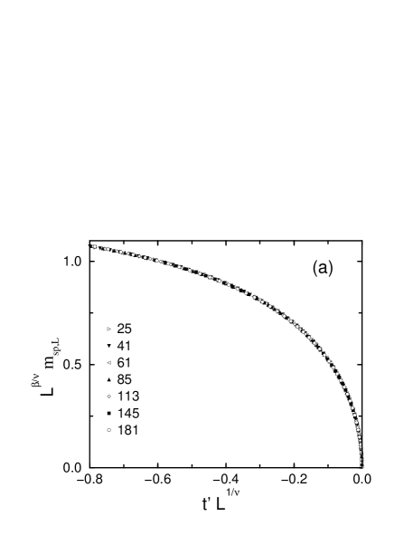
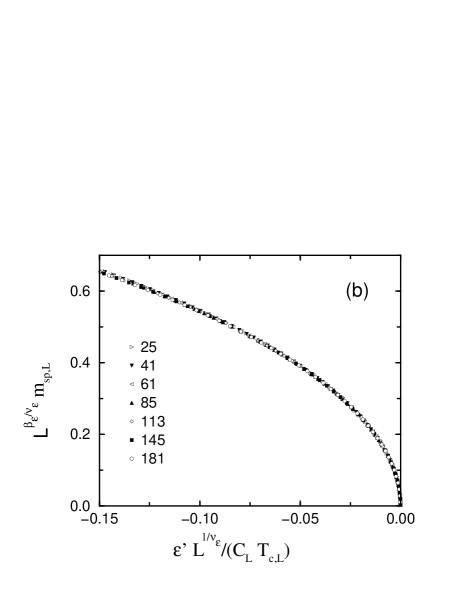
FIG. 8.: Scaled magnetisations of Ising clusters defined on a square lattice, see Fig. 2, as function of different scaling variables: (a) in the temperature picture, see Eq. (43), and (b) in the energy picture, see Eq. (61). The best data collapse yields the following values for the critical exponents: (a) $\beta=0.127$, $\nu=1.01$, (b) $\beta_{\varepsilon}=0.124$, $\nu_{\varepsilon}=1.02$.

Fig. 9 displays the scaled susceptibilities as function of the scaled reduced temperature. The values of the critical exponents $\gamma=1.77$ (to be compared with the exact value $\gamma_{ex}=1.75$) and $\nu=1.01$ again result from the best collapse of the scaled data. The same can be done in the energy picture where we obtain $\gamma_{\varepsilon}=1.80$ and $\nu_{\varepsilon}=1.02$, in reasonable agreement with the exact values. This shows that the finite size scaling theory enables us to obtain reliable values for critical exponents also in cases where an analysis of effective exponents does not succeed.

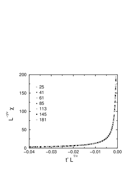
FIG. 9.: Scaled susceptibilities obtained for square lattice Ising clusters in the cluster molecular field approximation, see Fig. 4, as function of the scaled reduced temperature. The values $\gamma=1.77$ and $\nu=1.01$ of the critical exponents result from the best data collapse.

At this stage we have to emphasise again that no non-universal quantities of the infinite system enter the molecular field finite size scaling theory. Especially, the exact location of the critical point is not needed. On the other hand, using the value of $\nu$ obtained from finite size scaling together with the pseudo-critical temperatures of the three largest systems listed in Table I, a remarkable good estimation of the critical temperature follows from Eq. (39): $k_{B}T_{c}/J_{I}=2.266$ in excellent agreement with the exact value $k_{B}T_{c}/J_{I}=2/\ln(1+\sqrt{2})\approx 2.269$.

Before closing this subsection, we note that almost identical estimates are obtained for critical quantities when studying the triangular model: $\beta=0.127$, $\beta_{\varepsilon}=0.125$, $\gamma=1.78$, $\gamma_{\varepsilon}=1.80$, $\nu=1.03$, $\nu_{\varepsilon}=1.03$, and $k_{B}T_{c}/J_{I}=3.631$ (exact: $3.634$). The discrepancies are somewhat larger for the square lattice clusters where the next-nearest neighbour interactions have also been taken into account. We obtain $\beta=0.120$ and $\gamma=1.86$, for example, analysing systems with up to 81 spins.

B Three-dimensional Ising model

When trying to extract critical quantities for the three-dimensional Ising model from the cluster molecular field approximation, we are faced with two difficulties: (1) only systems with a very small number of spins ($\leq 57$) can be handled exactly and (2) the various clusters have different geometries, as explained in Section II. Especially the second point makes a finite size scaling analysis much more problematic, as discussed below. But let us start again by looking at the effective exponent derived from the spontaneous magnetisation. Fig. 10 shows the extrapolated exponent obtained for the different system sizes. The estimated value of 0.316 for the critical exponent $\beta$ is slightly smaller than the expected value $0.326$. This is due to the finite-size effects which for our small systems set in already at rather low temperatures. Fig. 10 also displays an oddity due to the different cluster geometries: on the dashed line the extrapolated exponents of two different system sizes, $N=27$ and $N=33$, are almost indistinguishable. Looking at the raw data, one observes that, by coincidence, due to the difference in the geometries, the cluster molecular field approximation yields virtually identical spontaneous magnetisations for these two clusters.

FIG. 10.: Extrapolated exponents $\beta_{ext,N}$ versus temperature for different three-dimensional Ising clusters defined on a cubic lattice. The quantities derived for systems with 27 and 33 spins are indistinguishable (indicated by the single dashed line).

The difficulties originating from the difference in geometry are enhanced when looking at the finite size scaling behaviour in three dimensions. In fact, the rather naive identification $L=N^{1/d}$, which works very well in two dimensions with identical geometries, is inadequate when different cluster geometries are involved. Sticking to this definition of $L$, we are only able to obtain simultaneously a good data collapse for all the quantities of interest (magnetisation and susceptibility as function of both reduced temperature and reduced energy) when the sizes $N=27$ and $N=33$ are omitted. This procedure then yields the following values for the critical exponents: $\beta=0.32$, $\beta_{\varepsilon}=0.41$, $\gamma=1.23$, $\gamma_{\varepsilon}=1.45$, $\nu=0.63$ and $\nu_{\varepsilon}=0.69$. Whereas in the temperature picture the values of the critical exponents agree nicely with the values given in the literature ($\beta=0.326$, $\gamma=1.24$, $\nu=0.63$), some discrepancies show up in the energy picture (for example, one expects 0.367 for $\beta_{\varepsilon}$), even if the overall agreement is still very satisfactory with regard to the smallness of our systems.

A possible way to circumvent some of the difficulties arising from the difference in cluster geometry would be to eliminate $L$ altogether in Eq. (43) resp. (56) by exploiting [7] the relation (39) resp. (57). However, this would introduce the necessity to determine precisely the location of the critical point beforehand.

An estimate of the critical exponent $\alpha$ of the infinite three-dimensional Ising system may be obtained by applying relation (50) for the maxima of the specific heat of the finite cluster systems. Using the system sizes 19 and 57 one obtains the value $\alpha=0.132$, again in reasonable agreement with the literature value $\alpha=0.109$.

In Section III we already discussed briefly the possible reduction of the correction to scaling terms when going from the temperature to the energy picture. Denoting the amplitude of the linear correction term in (55) by

$$K_{L}=L^{-\alpha/\nu}\frac{1}{a}(B_{L}-b_{L})$$ (65)

the ratio $B_{L}/K_{L}$ may serve as a measure of the suppression of the linear correction term in (55) compared to the corresponding term in (48). Note that the pseudo-critical temperature is not integrated into this ratio as $T_{c,L}$ appears in the scaling variable of the energy picture. For the magnetisation of the three-dimensional clusters this ratio is of the order 8. Similarly the ratio $B_{L}/(B_{L}-b_{L})$ describes the reduction of the correction term for a system with a logarithmically diverging specific heat. Again the factors appearing in the scaling variable of (61) are excluded from the ratio. For the two-dimensional Ising system in the cluster molecular field approximation this ratio is of the order 6. In both cases the corrections to scaling are suppressed in the energy picture as expected from the considerations in Section III. It is also observed in our data that the suppression decreases slightly with increasing system size for the range of extensions $L$ investigated in our cluster molecular field approximation.

Finally, we again get a very good estimate of the critical temperature from Eq. (39). Inserting the value $\nu=0.63$ coming from the best data collapse of the scaled data as well as the pseudo-critical temperatures of the systems with 7, 19, and 57 spins, we find $k_{B}T_{c}/J_{I}=4.5208$ which should be compared to the literature value $k_{B}T_{c}/J_{I}=4.5115$.

C Three-state Potts models

Let us close this Section by discussing three-state Potts models on square and triangular lattices. In these cases the cluster molecular field approximation displays a discontinuous transition for all finite clusters, as illustrated in Fig. 3 by the jump of the order parameters. At first sight this fact seems to rule out the possible determination of critical quantities from our small systems. However, we show in the following that our methods of analysing the data in principle still allow us to obtain reliable values for the critical quantities.

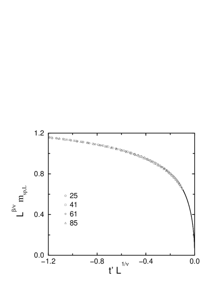
FIG. 11.: Scaled magnetisations of Potts clusters defined on a square lattice, see Fig. 3, as function of the reduced temperature scaling variable. Real data are shown by symbols, data obtained from a prolongation of the polynomial fits to $m_{sp}=0$, see main text, by the full lines. The best data collapse is achieved for the critical exponent values $\beta=0.11$ and $\nu=0.76$.

In the present situation the analysis of effective critical exponents has the great advantage that only data computed for temperatures lower than the critical temperature of the infinite system are involved. Therefore the discontinuous behaviour of our small systems observed at temperatures above the critical temperature does in this case not interfere with the determination of the critical exponents. Thus the extrapolated critical exponents computed for square lattice systems with up to 85 spins yield the value $\beta=0.104$ for the order parameter critical exponent, in good agreement with the exact value $\beta_{ex}=1/9$. On the other hand the molecular field finite size scaling analysis is deeply affected by the discontinuity of the phase transitions as here data obtained in close vicinity to the transition points play a prominent role. In fact, the main problem lies in the values of the pseudo-critical temperatures which enter the definition of the scaling variables. Using the transition temperatures given by the kinks in the cluster molecular field free energies, see inset of Fig. 3, does not lead to a collapse of the scaled data. A better result is obtained by fitting the spontaneous magnetisations of the finite systems to polynomials of second order and then inserting the temperatures where these polynomial functions hit the temperature axis into the scaling variables. This approach leads to an acceptable data collapse for the order parameter, as shown in Fig. 11, the critical exponents thereby taking the values $\beta=0.11$ and $\nu=0.76$. The value of $\beta$ again nicely agrees with the exact result but a slight discrepancy prevails for $\nu$ as the exact value is 5/6. With regard to the crudeness of our approach, this is still a very satisfactory result. However, we did not succeed in extracting the critical exponent $\gamma$ from the susceptibility data in a similar way. Finally, inserting the value $\nu=0.76$ into Eq. (39) together with the temperatures obtained from the polynomial fits, we end up with the estimate $k_{B}T_{c}/J_{P}=0.998$ for the critical temperature, very close to the exact value $k_{B}T_{c}/J_{P}=1/\ln(\sqrt{3}+1)\approx 0.995$.

V Conclusion

The advantages and shortcomings of molecular field theory are well known. On the one hand this approximation provides a rather simple way of obtaining analytical results even in complicated systems. Usually, the results of the molecular field approximation are qualitatively correct. On the other hand, however, large quantitative discrepancies are found when comparing these predictions with exact results or with estimations obtained by numerical methods and/or more sophisticated analytical approaches. This is especially the case when considering systems with a continuous phase transition as the molecular field approximation always yields classical values for the critical exponents irrespective of, for example, the dimensionality of the system. Furthermore, critical temperatures are usually overestimated by a considerable amount.

In this work we have shown that the correct values of critical quantities can nevertheless be obtained from systematic improvements of the molecular field approximation. We thereby insert spin clusters of variable sizes into a homogeneously magnetised background and determine the molecular field acting exclusively on the border spins by imposing a condition of homogeneity in the central part of the cluster. The interactions inside the clusters are treated exactly by computing the density of states as function of the internal energy and of the interaction energy with the molecular field.

The data computed in this cluster molecular field approximation can then be analysed in various ways in order to extract the values of critical quantities. We have discussed in this work two rather complementary approaches, one approach involving effective critical exponents where only data located at temperatures below the critical temperature of the infinite system enter, the other being a molecular field finite size scaling theory (which in the temperature picture is related to that developed by Suzuki [6, 7, 8, 9, 10, 11]) where the true critical exponents result from the best collapse of the rescaled data. In the latter approach the data located in close vicinity to the pseudo-critical temperatures are of main interest.

With these methods data resulting from the cluster molecular field treatment of various two- and three-dimensional Ising models as well as of two-dimensional three-state Potts models have been investigated. In all these cases we have shown that critical temperatures and critical exponents can be determined with a surprisingly high precision with regard to the smallness of our spin clusters. In two dimensions we have the nice situation that clusters of various sizes with the same shape can be handled by the available computational capacities. This is different in three dimensions where our computational resources do not allow us to handle spin clusters of various sizes having the same geometry. In fact, these restrictions are imposed by our choice to compute the density of states in a numerically exact manner. In principle larger system sizes could be investigated by Monte Carlo simulations, using one of the highly efficient methods for computing the density of states which have been developed recently [17]. However, very good numerical data would be needed in order to obtain the strength of the molecular field as a function of the temperature from Eq. (18). Especially the accurate determination of the pseudo-critical temperature requires a density of states of extremely high precision not easily achievable in a computer simulation. We therefore expect that data obtained from Monte Carlo simulations may not permit a molecular field finite size scaling analysis. However, they should be very useful for the investigations of effective critical exponents, especially when dealing with quantities like the susceptibility or the specific heat for which the small systems considered in this work did not allow a determination of the values of the critical exponents.

Further progress along the lines developed here can be achieved by noting that the homogeneity condition in the central part of the cluster renders our cluster molecular field approximation superior to more traditional approaches. However, the spin expectation value is still not identical in the whole cluster. Here a scheme developed by Galam [12] could be very useful. In that cluster molecular field scheme a cluster consisting of the central spin and of its $z$ neighbours is constructed such that the homogeneity is extended to the whole cluster. It is, however, not immediately obvious how to generalise this scheme to larger clusters containing not only the central spin and its nearest neighbours. Nevertheless we expect that the construction of homogeneously magnetised clusters (be it by the Galam scheme or by a different one) would further improve the systematic cluster molecular field approximation and yield even better values for the critical quantities.

Appendix

In this appendix we describe how the density of states is evaluated in a numerically exact way. For simplicity consider a square lattice which consists of $L$ rows of length $L$. In our case the density of states depends on two extensive quantities, the interaction energy $E$ of the spins inside the cluster and the interaction energy $B$ of border spins with spins $\sigma_{k}=1$ outside the cluster. In other physical contexts the density of states can depend on other extensive quantities, e.g. the interaction energy and the magnetisation. The density of states $\Omega(E,B)$ of the cluster is worked out by successively performing the trace over the $q^{L}$ states of a row of spins. A similar method has already been discussed in the literature for a density of states depending only on one extensive parameter [24, 25, 26]. Let $k=1,\ldots,q^{L}$ denote the configurations of the row of spins and $l=1,\ldots,L$ the rows of the cluster. Suppose $l$ rows of the cluster are already built up and the density of states of the incomplete cluster is given by $\omega_{l}(k,E,B)$. If the next row is added additional internal and external interactions of this row with the already built up cluster and the spins outside have to be included. Let ${\mathcal{E}}_{k^{\prime},k}$ denote the interaction energy of the microstate $k^{\prime}$ of the last row of the yet incomplete cluster with the microstate $k$ of the row to be added in the next step. Similarly ${\mathcal{B}}_{k}$ denotes the additional external energy. Of course ${\mathcal{B}}_{k}$ does not contain the contributions of those bonds of the new row which will become internal bonds when the next row is added. Then the density of states of the extended cluster consisting now of $l+1$ rows is given by

$$\omega_{l+1}(k,E,B) = \sum_{k^{\prime},E^{\prime},B^{\prime}}\omega_{l}(k^{\prime},E^{\prime},B^{\prime})$$ (67)

$$\delta(E,E^{\prime}+{\mathcal{E}}_{k^{\prime},k})\delta(B,B^{\prime}+{\mathcal{B}}_{k})\;.$$

The density of states of the complete cluster is then obtained as

$$\Omega(E,B)=\sum_{k}\omega_{L}(k,E,B)\;.$$ (68)

The described method is easily generalised to densities of states depending on more than two parameters.

REFERENCES

- [1] P. Weiss, J. Phys. Rad., Paris 6, 667 (1907).
- [2] H. A. Bethe, Proc. Roy. Soc. London A150, 552 (1935).
- [3] R. E. Peierls, Proc. Cambridge Philos. Soc. 32, 477 (1936).
- [4] P. R. Weiss, Phys. Rev. 74, 1493 (1948).
- [5] H. Müller-Krumbhaar and K. Binder, Z. Physik 254, 269 (1972).
- [6] M. Suzuki, Phys. Lett. 116A, 375 (1986).
- [7] M. Suzuki and M. Katori, J. Phys. Soc. Jpn. 55, 1 (1986).
- [8] M. Suzuki, J. Phys. Soc. Jpn. 55, 4205 (1986).
- [9] M. Suzuki, M. Katori, and X. Hu, J. Phys. Soc. Jpn. 56, 3092 (1987).
- [10] M. Katori and M. Suzuki, J. Phys. Soc. Jpn. 56, 3113 (1987).
- [11] X. Hu, M. Katori, and M. Suzuki, J. Phys. Soc. Jpn. 56, 3865 (1987).
- [12] S. Galam, Phys. Rev. B 54, 15991 (1996).
- [13] G. Kamieniarz, R. Dekeyser, G. Musiał, L. Dȩbski, and M. Bieliński, Phys. Rev. E 56, 144 (1997).
- [14] F. Y. Wu, Rev. Mod. Phys. 54, 235 (1982).
- [15] T. Kihiara, Y. Midzuno, and J. Shizume, J. Phys. Soc. Jpn. 9, 681 (1954).
- [16] L. Mittag and M. J. Stephen, J. Phys. A 7, L109 (1974).
- [17] A. Hüller and M. Pleimling, Int. J. Mod. Phys. C, in print, cond-mat/0110090.
- [18] M. N. Barber, Finite-Size Scaling, in Phase transition and Critical Phenomena (C. Domb and M. S. Green, eds.), Vol. 8, p. 145, London (1983).
- [19] M. Promberger and A. Hüller, Z. Phys. B 97, 341 (1995).
- [20] A. E. Ferdinand and M. E. Fisher, Phys. Rev. 185, 832 (1969).
- [21] M. Pleimling and W. Selke, Eur. Phys. J. B 1, 385 (1998).
- [22] B. M. McCoy and Tai Tsun Wu. The Two-Dimensional Ising Model. Harvard University Press (Cambridge, Mass., 1973).
- [23] S. M. Bhattacharjee and F. Seno, J. Phys. A: Math. Gen. 34, 6375 (2001).
- [24] K. Binder, Physica 62, 508 (1972).
- [25] R. J. Creswick, Phys. Rev. E 52, 5735 (1995).
- [26] R. J. Creswick and S.-Y. Kim, Phys. Rev. E 56, 2418 (1997).