Spin-polarized stable phases of the 2-D electron fluid at finite temperatures.

Abstract

The Helmholtz free energy $F$ of the interacting 2-D electron fluid is calculated nonperturbatively using a mapping of the quantum fluid to a classical Coulomb fluid $[$Phys. Rev. Letters, 87, 206 (2002)$]$. For density parameters $r_{s}$ such that $\sim 25<r_{s}$, the fluid is unpolarized at all temperatures $t=T/E_{F}$, where $E_{F}$ is the Fermi energy. For lower densities, the system becomes fully spin polarized for $t$ smaller than $\sim 0.35$, and partially polarized for $\sim 0.35<t<2$, depending on the density. At $r_{s}\sim 25-30$, and $t\sim 0.35$, an ”ambispin” phase where $F$ is almost independent of the spin polarization is found. These results support recent claims, based on quantum Monte Carlo results, for a stable, fully spin-polarized phase at $T$ = 0 for $r_{s}$ larger than $\sim 25-26$.

Introduction. The physics of the uniform two-dimensional electron gas (2DEG) depends crucially on the “coupling parameter” $\Gamma$ = (potential energy)/(kinetic energy) arising from the Coulomb interactions. The $\Gamma$ for the 2DEG at $T=0$ and mean density $n$ is equal to the mean-disk radius $r_{s}=(\pi n)^{-1/2}$ per electron. In the absence of a magnetic field or disorder effects, the density parameter $r_{s}$, the spin polarization $\zeta$ and the temperature $T$ are the only relevant physical variables. As the coupling constant increases, the 2DEG becomes more like a “liquid”, but here we continue to loosely call it an electron “gas”. A knowledge of the phase diagram at arbitrary $r_{s}$, $\zeta$ and $T$ is of crucial importance to a clear understanding of many intriguing phenomena (metal-insulator transitionrevmod , 2-D electrons in CuO layers, spin-dependent processes etc.) associated with the 2DEG.

A number of recent studiesvarsen ; atta ; prl2 have suggested that the 2DEG at $T$ =0 becomes fully spin-polarized for $r_{s}>r_{c}$ with $r_{c}\sim 25-30$. However the energy difference between the unpolarized and polarized phases is very close to the statistical uncertainty of the methods used. We have completed a study of this transition at finite temperatures where the energy differences for a larger data base become more significant and reveal a rich phase diagram which is fully consistent with the claimed $T=0$ polarized-fluid regime. It turns out that the partially degenerate strongly correlated 2DEG supports partially spin-polarized phases. This is particularly interesting since the 3DEG has also been recently shown to have partially spin-polarized stable phasesichi3dphase

The finite-$T$ phase diagram is examined using a computationally simple, conceptually novel method for calculating the quantum-PDFs and other properties (e.g, static response). The method has been applied to the 2DEGprl2 , the 3DEGprl1 ; prb00 , and hydrogen fluidshyd , at arbitrary coupling, spin polarization and temperature. It is based on identifying a “quantum temperature” $T_{q}$ such that the correlation energy of the corresponding classical Coulomb fluid at $T_{q}$ is equal to that of the quantum fluid at $T=0$. After that, hypernetted-chain (HNC) methods are used for the classical fluid. This classical mapping of quantum fluids within the HNC was named the CHNC. The application of the CHNC method to the 2DEG required the inclusion of short-range correlation effects (“bridge terms”) going beyond the usual HNC approximation. The resulting CHNC procedure for the 2DEG proved to be remarkably accurateprl2 . In fact even an application of CHNC at $T$ = 0, and without bridge corrections was examined by Bulutay and Tanatar and found to be very usefulbalutay .

We use Hartree atomic units, and consider a unit area $A$ with $n$ particles per unit area, with $n$ = $1/(\pi r_{s}^{2})$. The number density of each spin species is $n_{i}=n(1+\sigma_{i}\zeta)/2$, where i=1,2 would indicate up or, down spins with $\sigma_{i}=\pm 1$. The spin polarization $\zeta$ = $(n_{1}-n_{2})/n$. The total Helmholtz free energy per unit area, $F$, has the form $F_{0}+F_{x}+F_{c}$, where $F_{0}$, $F_{x}$, $F_{c}$ are the non-interacting, first-order exchange, and correlation, contributions to $F$. Thus all effects beyond first-order exchange are lumped into $F_{c}$, a convention used in density functional theory (DFT). The DFT exchange-correlation free energy would hence be $F_{xc}$ = $F_{x}+F_{c}$. In indicating spin-components we use the notation $F_{i}^{0},F_{i}^{x}$, and $F_{i}^{c}$ etc. The canonical ensemble is used so that the Helmholtz free energy is directly determined, unlike in the approach where the grand-potential $\Omega$ is determined in terms of the chemical potential which has to be inverted to obtain the density. This means $F_{0}$ and $F_{x}$ (being the first-order exchange) are determined in terms of the non-interacting chemical potential $\mu_{0}$, while $F_{c}$ has to be determined via a coupling constant integration, as discussed by us in ref prb00 ; pdw84 and in Dundrea et aldundrea .

The non-interacting free energy. Isihara and others have considered the expansion of the free energy about $T=0$ and obtained the leading terms in $r_{s}$, and $T$ isihara . However, the thermodynamic functions near $T=0$ have a particularly unfavourable structure for constructing such expansions. Since our calculations are nonperturbative, we evaluate $F_{0}$ etc., numerically, without expansion.

Using the the relation, $F_{0}=E_{0}-TS_{0}$, where $E_{0}$ and $S_{0}$ are the noninteracting internal energy and the entropy, $F_{0}$ can be calculated. An independent evaluation is obtained from the relation $F_{0}=n\mu_{0}-E_{0}$. Also, at $T=0$, we have, in Hartrees

$$F_{i}^{0}/n=E_{i}^{0}/n=(1+\sigma_{i}\zeta)^{2}/4r_{s}^{2}$$ (1)

Defining the Fermi function $f(e)=1/(1+exp(\beta e-\eta))$ where $\beta=1/T$, $\eta=\mu^{0}/T$,

$$n_{i} = (T/2\pi)I_{0}(\eta_{i})$$ (2)

$$E_{i} = (T^{2}/pi)I_{1}(\eta_{i})$$ (3)

$$F_{i}^{0} = n_{i}\mu_{i}^{0}-E_{i}^{0}$$ (4)

where the Fermi integral $I_{\nu}(z)$ is defined as

$$I_{\nu}(z)=\int_{0}^{\infty}\frac{dxx^{\nu}}{1+e^{x-z}}$$ (5)

The $I_{0}$ integral can be evaluated explicitly to give:

$$\eta_{i} = log[exp(1/t_{i})-1],\,\,t_{i}=E_{i}^{F}/T$$ (6)

$$E_{i}^{F} = E_{F}(1+\sigma_{i}\zeta),\,\,E_{F}=\pi n$$ (7)

The $I_{1}$ integral can be evaluated directly or reexpressed in terms of the dilogarithm function. We have evaluated $F_{0}$ by several methods; the dilog function was evaluated using the CERN library routine.

The exchange contribution to the free energy. The first-order unscreened exchange free energy $F_{x}$ consists of $F_{x}^{i}$, where $i$ denotes the spin species. At $T=0$ these reduce to the exchange energies:

$$E_{i}^{x}/n=-\frac{8}{3\surd{\pi}}n_{i}^{1/2}$$ (9)

Hence,

$$E_{x}/n=(E_{1}^{x}+E_{2}^{x})/n=-\frac{8}{3\pi r_{s}}[x_{1}^{3/2}+x_{2}^{3/2}]$$ (10)

where $x_{1}$ and $x_{2}$ are the fractional compositions $(1\pm\zeta)/2$ of the two spin species. At finite $T$, we have:

$$F_{i}^{x}/E_{i}^{x}=\frac{3}{16}t_{i}^{3/2}\int_{-\infty}^{\eta_{i}}\frac{I^{2}_{-1/2}(u)du}{(\eta_{i}-u)^{1/2}}$$ (11)

Here $I_{-1/2}$ is the Fermi integral. The total exchange free energy is $F_{x}=\Sigma F_{i}^{x}$. The accurate numerical evaluation of Eq. 11 requires the removal of the square-root singularity by adding and subtracting, e.g, $I^{2}(-|\eta|)/(v-|eta|)^{1/2}$ for the case where $\eta$ is negative, and $v=u$, and so on.

A real-space formulation of $F_{x}$ = $F_{1}^{x}+F_{2}^{x}$ using the zeroth-order PDFs fits naturally with the CHNC approach. Thus

$$F_{x}/n=n\int\frac{2\pi rdr}{r}\sum_{i<j}h^{0}_{ij}(r)$$ (12)

Here $h^{0}_{ij}(r)=g^{0}_{ij}(r)-1$. In the non-interacting system at temperature $T$, the antiparallel $h^{0}_{12}$, viz., $g_{12}^{0}(r,T)-1$, is zero while

$$h_{11}^{0}({\bf r})=-\frac{1}{n_{i}^{2}}\Sigma_{{\bf k}_{1},{\bf k}_{2}}n(k_{1})n(k_{2})e^{i({\bf k}_{1}-{\bf k}_{2}){\bf\cdot}{\bf r}}\,\,=\,-[f(r)]^{2}$$

Here k,r are 2-D vectors and $n(k)$ is the Fermi occupation number at the temperature $T$. At $T=0$ $f(r)=2J_{1}(k_{i}r)/k_{r}$ where $J_{1}(x)$ is a Bessel function. We have numerically evaluated the exchange free energy by both methods,i.e, Eq. 11 and Eq. 12, as a numerical check.

Correlation free energy. The correlation contribution, $F_{c}$ is evaluated together with the exchange contribution $F_{x}$ via a coupling constant integration over the distribution functions as follows:

$$F_{xc}/n=\int_{0}^{1}d\lambda n\int\frac{2\pi rdr}{r}\sum_{i<j}h_{ij}(r,\lambda)$$ (13)

Thus we need the interacting PDFs $g_{ij}(r,\lambda)$ for each $r_{s}$, $\zeta$ and $T$ for a number of values (we have used 7 values) of the coupling constant $\lambda$. The PDFs were evaluated using the CHNC method, as described in Ref.[prl2, ]. We present a brief summary of the CHNC method in the context of the present study.

Brief summary of the CHNC method. The essence of the CHNC method is to start from the quantum mechanical $g^{0}(r)$ of the non-interacting problem and build up the interacting $g(r)$ by classical methods.

The fluid of mean density $n$ contains two spin species with concentrations $x_{i}$ = $n_{i}/n$. While $T$ is the physical temperature of the 2DEG, we consider a classical fluid of temperature $T_{cf}$ = $1/\beta_{cf}$. Since the leading dependence of the energy on temperature is quadratic, we assume that $T_{cf}$= ${\surd{(T^{2}+T_{q}^{2})}}$ where $T_{q}$ is the quantum correction. This is clearly valid for $T=0$ and for high $T$, and was justified in more detail in ref. prb00, . The “quantum temperature” $T_{q}$ was shown to be given byprl2 ,

$$t=T_{q}/T_{F}=2/[1+0.86413(r_{s}^{1/6}-1)^{2}]$$ (14)

where the Fermi temperature $T_{F}$ is simply the Fermi energy $E_{F}=1/r_{s}^{2}$ in our units. In effect $T_{q}$ is really a single-parameter representation of the density-functional 2D correlation energy.

The HNC equations for the PDFs of a classical fluid, and the Ornstein-Zernike(OZ) relations arehncref :

$$g_{ij}(r) = exp[-\beta_{cf}\phi_{ij}(r)+h_{ij}(r)-c_{ij}(r)+B_{ij}(r)]$$

$$h_{ij}(r) = c_{ij}(r)+\Sigma_{s}n_{s}\int d{\bf r}^{\prime}h_{i,s}(|{\bf r}-{\bf r}^{\prime}|)c_{s,j}({\bf r}^{\prime})$$ (15)

This equation involves two quantities, viz., (i) the pair-potential $\phi_{ij}(r)$, (ii) the bridge function $B_{ij}(r)$rosen ; yr2d . The other terms, e.g, $c(r)$, is the “direct correlation function” of the OZ equations, while $h_{ij}(r)$ = $g_{ij}(r)$-1.

Pair-potential. The $\phi_{ij}(r)$ is the pair potential between the species $i,j$. For two electrons this is just the Coulomb potential $V_{cou}(r)$. If the spins are parallel, the Pauli principle prevents occupation of the same spatial orbital. This effect is equivalent to a “Pauli exclusion potential”, ${\cal P}(r)$ which when used in the HNC equation reproduces the $g^{0}_{ij}(r)$. Thus $\phi_{ij}(r)$ becomes ${\cal P}(r)\delta_{ij}+V_{cou}(r)$. The Coulomb potential $V_{cou}(r)$ for a pair of point-charge electrons is $1/r$. However, an electron at the temperature $T_{cf}$ is localized to within a thermal wavelength. Thus, we use a “diffraction corrected” form

$$V_{cou}(r)=(1/r)[1-e^{-rk_{th}}]$$ (16)

In the case of the 2DEG $k_{th}$ was explicitely determined by numerically solving the Schrodinger equation for a pair of 2-D electrons in the potential $1/r$ and calculating the electron density in each normalized statepdwkth . That is, by solving the 2-D Schrodinger equation (only $s\,$-waves are needed for the $r\to 0$ case):

$$\frac{d^{2}R}{dr^{2}}+\frac{1}{r}\frac{dR}{dr}+2m^{*}(\frac{k^{2}}{2}-\frac{1}{r})R=0$$ (17)

Here $m^{*}$ = 1/2 is the effective mass of the electron pair. The radial function has the asymptotic form:

$$R(r,k)\to[\frac{2}{\pi kr}]^{1/2}cos(kr-\frac{m^{*}}{k}ln(r)+\delta_{2d})$$ (18)

The “on-top” density $n(0)$ for electrons at the temperature $1/\beta$ is:

$$\frac{n(0)}{n}=\frac{\int^{\infty}_{0}k^{2}dkexp(-\beta k^{2}/2m^{*})R^{2}(0,k)}{\int^{\infty}_{0}k^{d}dkexp(-\beta k^{2}/2m^{*})}$$ (19)

Using the same form for the diffraction correction, i.e., $V_{d}(r)$=exp$(-k_{th}r)/r$, it was found that

$$k_{th}/k^{0}_{th}=1.158T_{cf}^{0.103}$$

where $T_{cf}$ is in a.u., and $k^{0}_{th}$ is the de Broglie thermal momentum $(2\pi m^{*}T_{cf})^{1/2}$.

Bridge contribution. The “bridge” term arises from higher-order cluster interactions. They seem to play a role similar to the “back-flow corrections” used in QMC trial wavefunctionskwon . Since the Pauli exclusion already acts to reduce clustering of parallel spin electrons, the $B_{ii}$ bridge corrections are unimportant. In Ref. prl2 we included the $B_{12}$ terms via a simple hard-disk bridge function,yr2d with a hard-disk packing fraction $\eta_{p}=0.1175r_{s}^{1/3}(T_{cf}/E_{F})$. Since $t=T_{cf}/E_{F}$ is itself a function of $r_{s}$, the zero temperature packing fraction $\eta_{p}(T=0)$ is just a function of $r_{s}$. In generalizing the above expression to finite $T$, we note that $r_{s}$ is simply the coupling constant $\gamma=P.E/K.E$ per electron. We take the potential energy $P.E$ = $1/r_{s}$ for a p͡air of electrons, and evaluate the kinetic energy ($K.E.$) from the non-interacting internal energy as in Eq. 2. Then the finite temperature hard-disk packing fraction is given by

$$\eta_{p}=0.235\gamma^{1/3}/[1+0.86413(\gamma^{1/6}-1)^{2}]$$ (20)

The next step is to use the $\phi_{ij}(r)$, and solve the coupled HNC+Bridge and OZ equations for the two-component interacting  fluid. Evaluation at several values of the coupling constant and integration as in Eq. 13 leads to the correlation free energy.

Figure 1: The phase diagram of the 2DEG as a function of the density parameter $r_{s}$ and temperature, showing fully and partially spin-polarized stable phases. The region near the dotted lines near $r_{s}\sim 25$ and $t\sim 0.35$ represents an ”ambispin” phase where the free energy is almost independent of the spin polarization.

Results. The fluid-phase with the lowest Helmholtz free energy $F(r_{s},T,\zeta)$ is the stable phase. We have evaluated $F$ for the range $t$ =$T/E_{F}<$ 2, and 5 $<r_{s}<40$, and usually for five values of $\zeta$ and found that the stable phase is the unpolarized (paramagnetic) phase for higher temperatures and densities. The initial suggestion of Varsano and Senatore that the 2DEG at $T$=0 is spin polarized near $r_{s}\sim 30$, and the more recent discussion by Attaccalite et al., that a transition occurs at $r_{s}$=25.7 are greatly strengthened by our results at finite-$T$. At $T$=0 we find a $\zeta=0\to\zeta=1$ transition at $r_{s}=r_{c}(\zeta:0\to 1)=26.7\pm 0.8$, but the stabilization energy is within the inherent uncertainities of the CHNC method. However, when taken together with all the results for neighbouring finite-$T$ values, a more plausible picture emerges ( Fig. 1). When the temperature is increased, the value of $r_{c}(\zeta:0\to 1)$ decreases somewhat and then begins to increase. However, when $t$ reaches $\sim 0.35$, partially polarized states with $\zeta\sim 0.7$ to 0.9 begin to compete for stability. This partially polarized state remains stable as long as the temperature is sufficiently low. An interesting aspect of the partially polarized regime is the existence of “ambi-spin” regions where the spin projection is NOT unambiguously determined since the energy differences as a function of the polarization are very small ( see below). For $t>\sim 1.5$, the stable phase becomes the usual unpolarized (paramagnetic) phase.

A plot of the energy difference $\Delta F(r_{s},t,\zeta)=F(\zeta)-F(0)$, as a function of the spin polarization is shown in Fig. 2 at several temperatures and $r_{s}$ values close to one of the transition lines. Thus the $t=0.05$ curve is at $r_{s}\sim 25.86$ which corresponds to $r_{c}(\zeta:0\to 1)$. This curve is similar to that given in Fig. 1 of Ref. atta . However, the the transition regions near $r_{s}\sim 26$ and $t\sim 0.35$ provides an example of a phase where the Helmholtz fee energy is almost independent of the spin polarization. Such an “ambispin phase” would be very sensitive to any external effects (impurities etc.,) that we have not considered in this study. The regions in Fig. 1 close to the dotted line, begining from the ”triangular” region near $r_{s}\sim 25$ and $t\sim 0.35$ are such regions. The partially spin polarized state is quite unusual since, in some regions, a very light deviation from $\zeta=1$ leads to a significantly large stability. Thus the curve at $t=0.5$ is typical of densities near $r_{s}\sim 30-32$ where the partially polarized stable is very close to unity but differs slightly from unity.

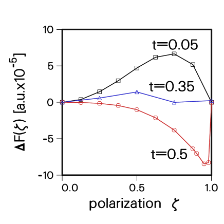
Figure 2: The polarization dependence of the Helmholtz free energy plotted as $\Delta F(\zeta)=F(r_{s},t,\zeta)-F(r_{s},t,0)$ at several temperatures and densities close to a tranition (see the text).

At $T=0$ the liquid phase becomes a Wigner crystal near $r_{s}\sim 35$. However, as the temperature is increased, this value will also increase. At low temperatures the crystal would be in equilibrium with the fully spin polarized phase. We have not investigated the equilibrium between the solid and liquid phases.

Thus the finite-$T$ 2DEG system provides many intriguing questions while complementing our understanding of the $T=0$ system. Our computer codes for generating the PDFs, the $f_{xc}((r_{s},T,\zeta)$ and related properties of the 2D electron fluid may prove to be useful for further studies of this system. The codes may be accessed via the internetweb .

In conclusion, we have evaluated the total Helmholtz free energy $F(r_{s},T,\zeta)$ = $F_{0}+F_{x}+F_{c}$, in the canonical ensemble, for a range of $r_{s}<$ 40, $t\leq 2$, and $0\leq z\leq 1$. The terms $F_{0}$ and $F_{x}$ were evaluated by several methods, without resorting to perturbation expansions, while the $F_{c}$ was evaluated via a coupling constant integration of the pair-distribution functions obtained from the CHNC equations. The finite-$T$ results are consistent with recent claims, based on quantum Monte Carlo calculations, of the existence of a fully spin-polarized stable phase at $T$ =0 and $r_{s}\sim 25-26$. Our results show that the finite-$T$ phase diagram of the clean, uniform 2DEG contains stable fully and partially spin-polarized phases. Ambispin phases where the free energy is quasi-independent of the spin polarization are also found. It is hoped that these results would stimulate new experiments and finite-$T$ QMC simulations.

References

- (1) electronic mail address: chandre@cm1.phy.nrc.ca
- (2) E. Abrahams, S. V. Kravchenko, and M. Sarachick, Rev. Mod. Phys. 73, 251 (2001)
- (3) D. Varsano et al., Europhys. Lett., 53, 348 (2001)
- (4) C. Attaccalite et al., Phys. Rev. Lett.88, 256601 (2002)
- (5) François Perrot and M. W. C. Dharma-wardana, Phys. Rev. Lett. 87, 206404 (2001)
- (6) D.P. Young et al, Nature (London) 397, 412 (1999), S. Ichimaru, Phys. Rev. Lett. 84, 1843 (1999)
- (7) M. W. C. Dharma-wardana and F. Perrot, Phys. Rev. Lett. 84, 959 (2000)
- (8) François Perrot and M. W. C. Dharma-wardana, Phys. Rev. B, 62, 14766 (2000)
- (9) M. W. C. Dharma-wardana and F. Perrot, Phys. Rev. B
- (10) C. Bulutay and B. Tanatar, Phys. Rev. B 65, 195116 (2002)
- (11) A. Isihara and T. Toyoda Phys Rev B, vol 21, p3358, 1980
- (12) F. Perrot and M.W.C. Dharma-wardana, Phys. Rev. A 30, 2619 (1984)
- (13) R. B. Dundrea et al, Phys. Rev. B 34, 2097 (1986)
- (14) J. M. J. van Leeuwen, J. Gröneveld, J. de Boer, Physica 25, 792 (1959)
- (15) F. Lado, S. M. Foiles and N. W. Ashcroft, Phys. Rev. A 26, 2374 (1983) Y. Rosenfeld, Phys. Rev. A 35, 938 (1987)
- (16) Y. Rosenfeld, Phys.Rev. A bf42, 5978 (1990), M. Baus et al., J. Phys. C: Solid State Phys. 19, L463 (1986)
- (17) François Perrot and M. W. C. Dharma-wardana, unpublished.
- (18) Y.Kwon et al., Phys. Rev. B 48, 12037 (1993)
- (19) http://nrcphy1.nrc.ca/ims/qp/chandre/chnc/