Kondo effect in quantum dots coupled to ferromagnetic leads

Abstract

We study the Kondo effect in a quantum dot which is coupled to ferromagnetic leads and analyse its properties as a function of the spin polarization of the leads. Based on a scaling approach we predict that for parallel alignment of the magnetizations in the leads the strong-coupling limit of the Kondo effect is reached at a finite value of the magnetic field. Using an equation-of-motion technique we study nonlinear transport through the dot. For parallel alignment the zero-bias anomaly may be split even in the absence of an external magnetic field. For antiparallel spin alignment and symmetric coupling, the peak is split only in the presence of a magnetic field, but shows a characteristic asymmetry in amplitude and position.

The Kondo effect hewson-book in electron transport through a quantum dot (QD) with an odd number of electrons is experimentally well established goldhaber ; kondo-odd . Screening of the dot spin due to the exchange coupling with lead electrons yields, at low temperatures, a Kondo resonance. The main goal of the present work is to investigate how ferromagnetic leads influence the Kondo effect. In the extreme case of half-metallic leads, minority-spin electrons are completely absent, i.e., the screening of the dot spin is not possible, and no Kondo-correlated state can form. What happens, however, for the generic case of partially spin polarized leads? How does the spin-asymmetry affect the Kondo effect? Is there still a strong coupling limit, and how are transport properties modified?

Based on a poor man’s scaling analysis we first show that the strong-coupling limit can still be reached in this case if an external magnetic field is applied. This is familiar from the Kondo effect in QDs with an even number of electrons sasaki ; cobden ; kondo-even-theory-1 ; kondo-even-theory-2 , which occurs at finite magnetic fields, although the physical mechanism is different in the present case. In the second part of the paper we analyze within an equation-of-motion (EOM) approach the nonlinear transport through the QD. We find that for parallel alignment of the lead magnetizations the zero-bias anomaly is split. This splitting can be removed by appropriately tuning the strength of an external magnetic field $B$. In the antiparallel configuration of the lead magnetizations no splitting occurs at zero field.

The Anderson Hamiltonian for a QD with a single level at energy $\epsilon_{0}$ coupled to ferromagnetic leads is

$$H = \sum_{rk\sigma}\varepsilon_{rk\sigma}c_{rk\sigma}^{\dagger}c_{rk\sigma}+\epsilon_{0}\sum_{\sigma}d_{\sigma}^{\dagger}d_{\sigma}+Ud_{\uparrow}^{\dagger}d_{\uparrow}d_{\downarrow}^{\dagger}d_{\downarrow}$$ (1)

$$+\sum_{rk\sigma}(V_{rk}d_{\sigma}^{\dagger}c_{rk\sigma}+V^{*}_{rk}c_{k\sigma}^{\dagger}d_{\sigma})+g\mu_{B}BS_{z}\;,$$

where $c_{rk\sigma}$ and $d_{\sigma}$ are the Fermi operators for electrons with wavevector $k$ and spin $\sigma$ in the leads, $r=L,R$, and in the QD, $V_{rk}$ is the tunneling amplitude, $S_{z}=(d_{\uparrow}^{\dagger}d_{\uparrow}-d_{\downarrow}^{\dagger}d_{\downarrow})/2$, and the last term is the Zeeman energy of the dot. (Stray fields from the leads are neglected.) We assume identical leads and symmetric coupling, $V_{Lk}=V_{Rk}$. The ferromagnetism of the leads is accounted for by different densities of states (DOS) $\nu_{r\uparrow}(\omega)$ and $\nu_{r\downarrow}(\omega)$ for up and down-spin electrons.

In the following we study the two cases of parallel (P) and antiparallel (AP) alignment of the leads’ magnetic moments. For the AP configuration and zero magnetic field and bias voltage, the model is equivalent (by canonical transformation glazman ) to a QD coupled to a single lead with DOS $\nu_{L\uparrow}+\nu_{R\uparrow}=\nu_{L\downarrow}+\nu_{R\downarrow}$. In this case, the usual Kondo resonance forms, which is the same as for nonmagnetic electrodes hewson-book .

This changes for the P configuration. In this case, there is an overall asymmetry for up and down spins, say $\nu_{L\uparrow}+\nu_{R\uparrow}>\nu_{L\downarrow}+\nu_{R\downarrow}$. To understand how this asymmetry affects the Kondo physics we apply the poor man’s scaling technique anderson , performed in two stages haldane . In the first stage, charge fluctuations dominate and lead to a renormalization of the QD’s levels. Since the renormalization for the spin-down level is stronger than for spin-up, a level splitting between the two spin orientations is generated. This is one of the key mechanism for all the effects discussed below. To reach the strong-coupling limit it is, therefore, essential to apply an external magnetic field to compensate for the generated spin splitting. In the second stage, the resulting model is mapped onto a Kondo Hamiltonian and the degrees of freedom involving spin fluctuations are integrated out. For simplicity we assume for the scaling analysis flat DOSs $\nu_{r\sigma}$ and neglect the $k$-dependence of the tunnel amplitudes $V_{rk}=V$.

First we reduce the cutoff $D$ from $D_{0}$, which is the smaller value of the bandwidth and the onsite repulsion $U$ haldane . Charge fluctuations lead to the scaling equations

$$\frac{d\epsilon_{\sigma}}{d\ln(D_{0}/D)}=\frac{\Gamma_{\bar{\sigma}}}{2\pi}$$ (2)

where we defined $\Gamma_{\sigma}=2\pi|V|^{2}\sum_{r}\nu_{r\sigma}$, and $\bar{\sigma}$ is opposite to $\sigma$. This yields the solution $\Delta\widetilde{\epsilon}=\widetilde{\epsilon}_{\uparrow}-\widetilde{\epsilon}_{\downarrow}=-(1/\pi)P\Gamma\ln(D_{0}/D)+\Delta\epsilon_{0}$, where $P=(\nu_{r\uparrow}-\nu_{r\downarrow})/(\nu_{r\uparrow}+\nu_{r\downarrow)}$ measures the spin polarization in the leads, $\Gamma=(\Gamma_{\uparrow}+\Gamma_{\downarrow})/2$ and $\Delta\epsilon_{0}=g\mu_{B}B$ is the Zeeman splitting. The empty-dot state $|0\rangle$ hybridizes with states where the dot is singly occupied $|1\sigma\rangle$ with either spin up or down, while the singly-occupied state $|1\sigma\rangle$ only hybridizes with the empty-dot state $|0\rangle$ (for $U\gg|\epsilon|$ - asymmetric Anderson model). Because of the spin-dependent DOS in the leads the hybridization is spin-dependent, which is the physical origin of the generated $\Delta\widetilde{\epsilon}$.

To describe Kondo physics (for $\widetilde{\epsilon}<0$) we terminate haldane the scaling of Eq. (2) at $\widetilde{D}\sim-\widetilde{\epsilon}$, and perform a Schrieffer-Wolff transformation. Using the renormalized parameters $\widetilde{D}$ and $\widetilde{\epsilon}$ we get the effective Kondo Hamiltonian

$$H_{\rm Kondo}=\sum_{rr^{\prime}kk^{\prime}}\{J_{+}S^{+}c^{{\dagger}}_{rk\downarrow}c_{r^{\prime}k^{\prime}\uparrow}+J_{-}S^{-}c^{{\dagger}}_{rk\uparrow}c_{r^{\prime}k^{\prime}\downarrow}+$$

$$S_{z}(J_{z\uparrow}c^{{\dagger}}_{rk\uparrow}c_{r^{\prime}k^{\prime}\uparrow}-J_{z\downarrow}c^{{\dagger}}_{rk\downarrow}c_{r^{\prime}k^{\prime}\downarrow})\}\,,$$ (3)

plus the term $-2S_{z}\tilde{D}(\nu_{\uparrow}J_{z\uparrow}-\nu_{\downarrow}J_{z\downarrow})$ and a potential scattering term. The initial values for the coupling constants are $J_{+}=J_{-}=J_{z\uparrow}=J_{z\downarrow}={|V|^{2}/|\widetilde{\epsilon}|}\equiv J_{0}$. To reach the strong-coupling limit we tune the external magnetic field $B$ such that the total effective Zeeman splitting vanishes, $\Delta\widetilde{\epsilon}=0$ (the field $B$ will also slightly modify the DOS in the leads kondo-even-theory-1 ). During the second stage of scaling spin fluctuations will renormalize the three coupling constants $J_{+}=J_{-}\equiv J_{\pm}$, $J_{z\uparrow}$, and $J_{z\downarrow}$ differently. The scaling equations are

$$\frac{d(\nu_{\pm}J_{\pm})}{d\ln(\widetilde{D}/D)} = \nu_{\pm}J_{\pm}(\nu_{\uparrow}J_{z\uparrow}+\nu_{\downarrow}J_{z\downarrow})$$ (4)

$$\frac{d(\nu_{\sigma}J_{z\sigma})}{d\ln(\widetilde{D}/D)} = 2(\nu_{\pm}J_{\pm})^{2}$$ (5)

with $\nu_{\pm}=\sqrt{\nu_{\uparrow}\nu_{\downarrow}}$, $\nu_{\sigma}\equiv\sum_{r}\nu_{r\sigma}$ com_models . To solve these equations we observe that $(\nu_{\pm}J_{\pm})^{2}-(\nu_{\uparrow}J_{z\uparrow})(\nu_{\downarrow}J_{z\downarrow})=0$ and $\nu_{\uparrow}J_{z\uparrow}-\nu_{\downarrow}J_{z\downarrow}=J_{0}P(\nu_{\uparrow}+\nu_{\downarrow})$ is constant as well. I.e., there is only one independent scaling equation. All coupling constants reach the stable strong-coupling fixed point $J_{\pm}=J_{z\uparrow}=J_{z\downarrow}=\infty$ at the Kondo energy scale, $D\sim k_{B}T_{K}$. For the P configuration the Kondo temperature in leading order,

$$T_{\rm K}(P)\approx\widetilde{D}\exp\left\{-{1\over(\nu_{\uparrow}+\nu_{\downarrow})J_{0}}\,{{\rm arctanh}(P)\over P}\right\}\;,$$ (6)

depends on the polarization $P$ in the leads. It is a maximum for nonmagnetic leads, $P=0$, and vanishes for $P\rightarrow 1$.

Finally, we point out an interesting consequence of the spin polarization in the leads. With nonmagnetic leads, the Kondo Hamiltonian couples the spin of the QD to the spin of the leads only, but not to its charge. To analyze the analogous situation in our case, we introduce the (pseudo) spin $\vec{\sigma}=(1/2)\sum_{kk^{\prime}rr^{\prime}\sigma\sigma^{\prime}}c^{\dagger}_{kr\sigma}\sigma_{\sigma\sigma^{\prime}}c_{k^{\prime}r^{\prime}\sigma^{\prime}}/(2\widetilde{D}\sqrt{\nu_{\sigma}\nu_{\sigma^{\prime}}})$, where the spin-dependent normalization factor is crucial to ensure the proper spin commutation relations, and the (pseudo) charge $en=e\sum_{kk^{\prime}rr^{\prime}\sigma}c^{\dagger}_{kr\sigma}c_{k^{\prime}r^{\prime}\sigma}/(2\widetilde{D}\nu_{\sigma})$. The last term in Eq. (3) can, then, be written as $2\widetilde{D}(\nu_{\uparrow}J_{z\uparrow}+\nu_{\downarrow}J_{z\downarrow})\sigma_{z}S_{z}$ plus $\widetilde{D}(\nu_{\uparrow}J_{z\uparrow}-\nu_{\downarrow}J_{z\downarrow})nS_{z}$. The first term is analogous to the Kondo model with nonmagnetic leads, while the second term couples spin to charge. The latter does not scale up and the associated additional renormalization of the Zeeman splitting, $-(1/\pi)P\Gamma$, is negligible as compared to $\Delta\widetilde{\epsilon}$ in the limit $D_{0}\gg|\epsilon|$.

The unitary limit for the P configuration can be achieved by tuning the magnetic field appropriately, as discussed above. In this case, the maximum conductance through the QD is $G_{{\rm max},\sigma}^{P}=e^{2}/h$ per spin, i.e., the same as for nonmagnetic leads. This yields that the amplitude of the Kondo resonance for up and down spin at the Fermi level are different, since $G_{{\rm max},\sigma}^{P}\sim\Gamma_{\sigma}(E_{\rm F})\rho_{\sigma}(E_{\rm F})$, and therefore, $\rho_{\uparrow}(E_{\rm F})/\rho_{\downarrow}(E_{\rm F})=(1-P)/(1+P)$. For the AP configuration, the maximal conductance is reduced, $G_{{\rm max},\sigma}^{AP}=(1-P^{2})e^{2}/h$, and vanishes for $P\rightarrow 1$.

In the remainder of this article we analyze the DOS of the QD and address nonequilibrium transport. For a qualitative discussion we should employ the simplest technique which accounts for both the formation of Kondo resonances and the influence of the spin-dependent renormalization of the dot level on spin fluctuations. The equation-of-motion (EOM) technique with the usual decoupling procedure meir ; EOM for higher order Green functions (GF) satisfies the first requirement but not the second. We, therefore, extend this scheme by calculating the level splitting $\Delta\widetilde{\epsilon}$ self-consistently. For a more quantitative analysis one could include higher-order (than usually) Green’s functions in the EOM approach or higher-order diagrams in the resonant-tunneling-approximation konig , or use more advanced schemes such as real-time konig2 or numerical RG costi1 methods. These techniques are, however, much more complex com_slaveboson and are not pursued here.

Within the Keldysh formalism, the transport current $I=\sum_{\sigma}I_{\sigma}$ through a QD for $\Gamma_{{\rm R}\sigma}(\omega)=\lambda_{\sigma}\Gamma_{{\rm L}\sigma}(\omega)$ is

$$I_{\sigma}=\frac{e}{\hbar}\int d\omega\frac{\Gamma_{{\rm L}\sigma}(\omega)\Gamma_{{\rm R}\sigma}(\omega)}{\Gamma_{{\rm L}\sigma}(\omega)+\Gamma_{{\rm R}\sigma}(\omega)}[f_{\rm L}(\omega)-f_{\rm R}(\omega)]\rho_{\sigma}(\omega)$$ (7)

where $\rho_{\sigma}(\omega)=-(1/\pi)\,{\rm Im}\,G^{\rm ret}_{\sigma}(\omega)$. For strong interaction ($U\rightarrow\infty$) the retarded Green’s function is

$$G^{\rm ret}_{\sigma}(\omega)=\frac{1-\langle n_{\bar{\sigma}}\rangle}{\omega-\epsilon_{\sigma}-\Sigma_{0\sigma}(\omega)-\Sigma_{1\sigma}(\omega)+i0^{+}}$$ (8)

where $\Sigma_{0\sigma}(\omega)=\sum_{k\in{\rm L,R}}|V_{k}|^{2}/(\omega-\varepsilon_{k\sigma})$ is the self-energy for a noninteracting QD, while

$$\Sigma_{1\sigma}(\omega,\Delta\widetilde{\epsilon})=\sum_{k\in{\rm L,R}}\frac{|V_{k}|^{2}f_{\rm L/R}(\varepsilon_{k\bar{\sigma}})}{\omega-\sigma\Delta\widetilde{\epsilon}-\varepsilon_{k\bar{\sigma}}+i\hbar/2\tau_{\bar{\sigma}}}$$ (9)

appears for interacting QDs only. The average occupation of the QD with spin $\sigma$ is obtained from $\langle n_{\sigma}\rangle=-(i/2\pi)\int d\omega\,G^{<}_{\sigma}(\omega)$. Extending the standard derivation meir , we replaced on the r.h.s. of Eq. (9) $\Delta\epsilon\rightarrow\Delta\widetilde{\epsilon}$, where $\widetilde{\epsilon}_{\sigma}$ is found self-consistently from the relation

$$\widetilde{\epsilon}_{\sigma}=\epsilon_{\sigma}+{\rm Re}[\Sigma_{0\sigma}(\widetilde{\epsilon}_{\sigma})+\Sigma_{1\sigma}(\widetilde{\epsilon}_{\sigma},\Delta\widetilde{\epsilon})]\,,$$ (10)

which describes the renormalized dot-level energy, where the real part of the denominator of Eq. (8) vanishes hewson-book . We emphasize that without this self-consistency relation the Kondo resonances will, in general, appear at different positions, which disagree with the conclusions from the scaling analysis sergueev . The procedure simulates higher-order contributions and the influence of the renormalization of the dot level on spin fluctuations. Following Ref. meir we introduce, in heuristic way, a lifetime $\tau_{\sigma}(\mu_{\rm L},\mu_{\rm R},\widetilde{\epsilon}_{\uparrow},\widetilde{\epsilon}_{\downarrow})$ which describes decoherence due to a finite bias voltage $V$ or level splitting $\Delta\widetilde{\epsilon}$. It is obtained in second-order perturbation theory and depends on the electrochemical potentials in the leads, $\mu_{\rm L(R)}$, and the level positions. Again, we replace the bare levels by the renormalized ones. In the numerical results presented below we use Lorentzian bands of width $D=100\Gamma$.

For nonmagnetic leads, $P=0$ and zero magnetic field, $B=0$, the proposed approximation is identical to the standard EOM scheme meir . For finite magnetic field, $B\neq 0$, the self-consistency condition yields a splitting of the Kondo resonances which is slightly smaller than $2g\mu_{B}B$, in agreement with both experimental goldhaber and theoretical findings moore ; costi2 . For $B=0$ and $P>0$ in the parallel configuration, we obtain a value of the splitting $\Delta\widetilde{\epsilon}$ comparable to the result from scaling, Eq. (2).

In Fig. 1 we plot the DOS of the QD for spins in AP and P configurations with spin polarization $P=0.2$ in the leads. In the AP configuration there is one Kondo resonance [Fig. 1(a)] and the DOS is the same as for the case of nonmagnetic leads. For the P configuration, however, the Kondo resonance splits [Fig. 1(c)], which can be compensated by an external magnetic field $B$ [Fig. 1(d)]. In the latter case, the amplitude of the Kondo resonance for spin down significantly exceeds that for spin up (as discussed above). A finite bias voltage, $\mu_{\rm R}-\mu_{\rm L}=eV>0$, again leads to a splitting for both the AP and the P configurations, [Fig. 1(b) and (e)]. In the AP configuration, the amplitude of the upper and the lower Kondo peak appear asymmetric [Fig. 1(b)].

In Fig. 2 we show the differential conductance as a function of the transport voltage. For nonmagnetic leads, there is a pronounced zero-bias maximum [Fig. 2(a)], which splits in the presence of a magnetic field [Fig. 2(b)]. For magnetic leads and parallel alignment, we find a splitting of the peak in the absence of a magnetic field [Fig. 2(c)], which can be tuned away by an appropriate magnetic field [Fig. 2(d)]. In the AP configuration, the opposite happens, no splitting at $B=0$ [Fig. 2(e)] but finite splitting at $B>0$ [Fig. 2(f)] with an additional asymmetry in the peak amplitudes as function of the bias voltage. This asymmetry is related to the asymmetry in the amplitude of DOS [Fig. 1(b)]. All these findings are in good agreement with our scaling analysis. In Fig. 2(g) we show the tunnel magnetoresistance (TMR) which can be much larger than for conventional TMR systems. Finally, we find that the positions of the peaks in the AP configuration in the presence of a magnetic field are slightly shifted as a function of the polarization $P$ [Fig. 2(h)]. This can be explained in the similar way as in Ref. kondo-even-theory-2 by an additional level splitting $\delta\Delta\widetilde{\epsilon}=(1/4\pi)\,P\,\Gamma/\widetilde{\epsilon}\,eV$ at finite bias voltages due to spin accumulation in the QD.

We finally comment on the observability of our proposal. Ferromagnetic systems usually have strong spin-orbit coupling which could lead to spin-flip relaxation and, thus, could destroy the Kondo effect. On the other hand, recent observation of Aharonov-Bohm oscillations in a ferromagnetic ring kasai proved coherent transport, i.e., the formation of the Kondo cloud in ferromagnetic leads might be possible as well. How can one attach ferromagnetic leads to a QD? A conceivable realization might be to put carbon nanotubes in contact to ferromagnetic leads ago . The Kondo effect has been observed already for nonmagnetic electrodes cobden ; bachtold . Alternatively one might use magnetic tunnel junctions with magnetic impurities in the barrier, or spin-polarized STM ralph ; wiesendanger .

In conclusion, we presented a qualitative study of the Kondo effect in QDs coupled to ferromagnetic leads. In particular we found a splitting of the Kondo resonance for parallel alignment of the leads magnetizations, even in the absence of a magnetic field. Our results are based on a poor man’s scaling approach and an EOM technique. Further investigations on a more quantitative level using more advanced techniques would be desirable.

We thank L. Borda, J. von Delft, L. Glazman, B. Jones, Yu.V. Nazarov, A. Rosch, H. Schoeller, A. Tagliacozzo, M. Vojta and A.Zawadowski for discussion. Support by the Research Project KBN 5 P03B 091 20 and the DFG through the CFN and the Emmy-Noether program is acknowledged.

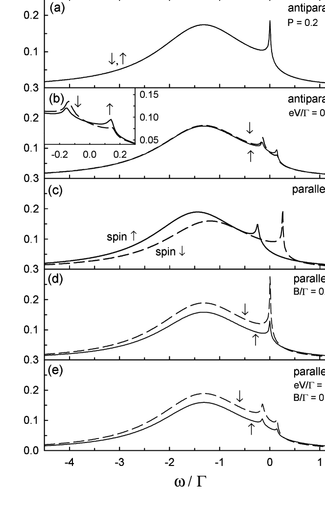
Figure 1: Spin dependent DOS for spin up (solid line) and spin down (dashed), calculated for P and AP alignment (as indicated), for a spin polarization of the leads $P=0.2$. The parts (d,e) include the effect of an applied magnetic field $B$ and (b,e) of an applied bias voltage $V$. The other parameters are: $T/\Gamma=0.005$ and $\epsilon/\Gamma=-2$.

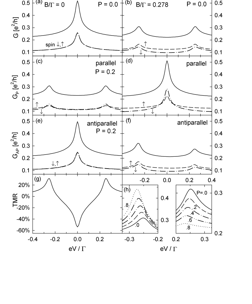
Figure 2: Total differential conductance (solid lines) as well as the contributions for spin up (dashed) and the spin down (dotted-dashed) vs. the applied bias voltage $V$ at zero magnetic field $B=0$ (a,c,e) and at finite magnetic field (b,d,f,h) for normal (a,b) and ferromagnetic leads with parallel (c,d) and antiparallel (e,f,h) alignment of the lead magnetizations. Part (g) shows the tunnel magnetoresistance, ${\rm TMR}=(G_{\rm P}-G_{\rm AP})/G_{\rm AP}$, for the cases (c) and (e). (h) The conductance $G_{\rm AP}/(1-P^{2})$ for several values of $P$ as indicated. Other parameters are as in Fig. 1

References

- (1) A. C. Hewson, The Kondo Problem to Heavy Fermions, Cambridge Univ. Press (1993).
- (2) D. Goldhaber-Gordon et al., Nature (London) 391, 156 (1998).
- (3) S. M. Cronenwett et al., Science 281, 540 (1998); F. Simmel et al., Phys. Rev. Lett. 83, 804 (1999); J. Schmid et al., Phys. Rev. Lett. 84, 5824 (2000); W. G. van der Wiel et al., Science 289, 2105 (2000).
- (4) S. Sasaki et al., Nature (London) 405, 764 (2000);
- (5) J. Nygård, D. H. Cobden, and P. E. Lindelof, Nature (London) 408, 342 (2000).
- (6) M. Pustilnik, Y. Avishai, and K. Kikoin, Phys. Rev. Lett. 84, 1756 (2000); M. Eto and Yu. V. Nazarov, Phys. Rev. B 64, 085322 (2001).
- (7) M. Pustilnik and L. I. Glazman, Phys. Rev. Lett. 85, 2993 (2000); Phys. Rev. B 64, 045328 (2001).
- (8) L. I. Glazman and M. E. Raikh, JETP Lett. 47, 452 (1988); T. K. Ng and P. A. Lee, Phys. Rev. Lett. 61, 1768 (1988).
- (9) P. W. Anderson, J. Phys. C 3, 2439 (1970).
- (10) F. D. M. Haldane, Phys. Rev. Lett. 40, 416 (1978).
- (11) We note that the (spin-dependent) DOS and the (spin-independent) tunneling amplitudes enter the scaling equations Eqs. (2), (4) and (5) only via the combination . As a consequence, all the conclusions drawn in this paper are valid also for a system with spin-dependent tunneling amplitudes but nonmagnetic leads.
- (12) Y. Meir, N. S. Wingreen and P. A. Lee, Phys. Rev. Lett. 70, 2601 (1993); N. S. Wingreen and Y. Meir, Phys. Rev. B 49, 11 040 (1994).
- (13) The approximations used here within the EOM scheme are rather crude. Its validity range is limited to temperatures above . In this regime, while quantitative precision for quantities such as the Kondo temperature and the occupation number are not achieved the main physical effects are well described (see Ref. meir and references therein).
- (14) J. König, J. Schmid, H. Schoeller, and G. Schön, Phys. Rev. B 54, 16 820 (1996).
- (15) The slave boson technique in the non-crossing approximation does not describe the influence of magnetic fields properly meir , whereas the mean field approximation overestimates the magnetic order, especially dorin for large , since it neglects quantum fluctuations.
- (16) V. Dorin and P. Schlottmann, Phys. Rev. B 47, 5095 (1993); J. Appl. Phys. 73, 5400 (1993).
- (17) H. Schoeller and J. König, Phys. Rev. Lett. 84, 3686 (2000).
- (18) T. A. Costi, A. C. Hewson, and V. Zlatić, J. Phys.: Cond. Mat. 6, 2519 (1994).
- (19) In [N. Sergueev et al., Phys. Rev. B 65, 165303 (2002)] the authors analyze the Anderson model by using an equations-of-motions scheme without the additional self-consistency assumption and found no splitting of zero-bias anomaly.
- (20) J. E. Moore, X-G. Wen, Phys. Rev. Lett. 85, 1722 (2000).
- (21) T. A. Costi, Phys. Rev. Lett. 85, 1504 (2000); Phys. Rev. B 64, 241310 (2001).
- (22) S. Kasai, T. Niiyama, E. Saitoh, and H. Miyajima, Appl. Phys. Lett. 81, 316 (2002).
- (23) K. Tsukagoshi, B. W. Alphenaar, and H. Ago, Nature (London) 401, 572 (1999).
- (24) M. R. Buitelaar, A. Bachtold, T. Nussbaumer, M. Iqbal, and C. Schönenberger, Phys. Rev. Lett. 88, 156801 (2002).
- (25) D. C. Ralph and R. A. Buhrman, Phys. Rev. Lett. 72, 3401 (1994).
- (26) A. Kubetzka, M. Bode, O. Pietzsch, and R. Wiesendanger, Phys. Rev. Lett. 88, 057201 (2002).