Photoemission in the High $T_{c}$ Superconductors

Summary.

We review angle resolved photoemission spectroscopy (ARPES) results on the high $T_{c}$ superconductors, focusing primarily on results obtained on the quasi-two dimensional cuprate Bi₂Sr₂CaCu₂O₈ and its single layer counterpart Bi₂Sr₂CuO₆. The topics treated include the basics of photoemission and methodologies for analyzing spectra, normal state electronic structure including the Fermi surface, the superconducting energy gap, the normal state pseudogap, and the electron self-energy as determined from photoemission lineshapes.

1 Introduction

Angle resolved photoemission spectroscopy (ARPES) has played a major role in the elucidation of the electronic excitations in the high temperature cuprate superconductors. Several reasons have contributed to this development. First, the great improvement in experimental resolution, both in energy and momentum, aided by the large energy scales present in the cuprates, allows one to see features on the scale of the superconducting gap. More recently the resolution has improved to such an extent, that now features in traditional superconductors like Nb and Pb, with energy scales of a meV, can be observed by ARPES Yokoya .

Second, most studies have focused on $Bi_{2}Sr_{2}CaCu_{2}O_{8}$ (Bi2212) and its single layer counterpart, $Bi_{2}Sr_{2}CuO_{6}$ (Bi2201). These materials are characterized by weakly coupled BiO layers, with the longest interplanar separation in the cuprates. This results in a natural cleavage plane, with minimal charge transfer. This is crucial for ARPES, since it is a surface sensitive technique; for the photon energies typically used, the escape depth of the outgoing electrons is only of the order of $\sim 10\AA$. For this reason, we elect to concentrate on these materials in the current article, since the data are known to be reproducible among the various groups.

The third reason is the quasi-two dimensionality of the electronic structure of the cuprates, which permits one to unambiguously determine the momentum of the initial state from the measured final state momentum, since the component parallel to the surface is conserved in photoemission. Moreover, in two dimensions, ARPES directly probes the the single particle spectral function, and therefore offers a complete picture of the many body interactions inherent in these strongly correlated systems.

There are other reasons to point out as well. For example, the very incoherent nature of the excitations near the Fermi energy in the normal state does not allow the application of traditional techniques, such as the de Haas van Alphen effect. The electrons simply do not live long enough to complete a cyclotron orbit. Another important reason why ARPES has played a major role is the highly anisotropic nature of the electronic excitations in the cuprates, which means that momentum resolved probes are desirable when attempting to understand these materials.

It is satisfying to compare the earlier ARPES papers to more recent ones, and observe the remarkable progress the field has undergone. But this satisfaction must be tempered by the knowledge that the current literature is still full of unresolved issues. Undoubtedly, some of what is described here will be viewed in a new light in the future, and we will try to point out the contentious points, but the reader must keep in mind that the writers, by necessity, approach this task with their own set of biases. For a complementary view, the reader is refered to the recent review by Damascelli, Shen and Hussain RMP . An earlier review of ARPES studies of high $T_{c}$ superconductors can be found in the book by Lynch and Olson LYNCH .

2 Basics of Angle-Resolved Photoemission

The basics of angle-resolved photoemission have been described in detail in the literatureHUFNER . We will limit ourselves to a brief review of some salient points, emphasizing those aspects of the technique which will be useful in understanding ARPES studies of high $T_{c}$ superconductors. We start by looking at a simple independent particle picture, and subsequently include the effects of strong interactions.

The simplest model of ARPES is the three step model 3STEP , which separates the process into photon absorption, electron transport through the sample, and emission through the surface. In the first step, the incident photon with energy $h\nu$ is absorbed by an electron in an occupied initial state, causing it to be promoted to an unoccupied final state, as shown in Fig. 1a. There is conservation of energy, such that

$$h\nu=BE+\Phi+E_{\rm kin}$$ (1)

where $\Phi$ is the work function, and $BE$ and $E_{\rm kin}$ are the binding and kinetic energies of the electron, respectively. We will not discuss the subsequent two steps of the three step model, photoelectron transport to the surface and transmission through the surface into the vacuum, as they only affect the number of emitted electrons, and thus the absolute intensity HUFNER .

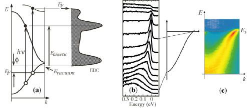
Figure 1: a: Independent particle approximation view of ARPES; To the right is the resulting energy distribution curve (EDC); b: Experimental EDCs along a path in momentum space in Bi2212; c: Intensity map from these data.

The kinetic energy of the electrons is measured by an electron energy analyzer. If the number of emitted electrons is then plotted as a function of their kinetic energy, as shown in Fig. 1, peaks are found whenever an allowed transition takes place. Eq. (1) then yields the kinetic energy of the electron if the work function is known. Measuring $\Phi$ accurately is not a trivial task, but fortunately, in the case of a metallic sample one does not need to know $\Phi$. By placing the sample in electrical contact with a good metal (e.g., polycrystalline gold) one can measure the binding energy in the sample with respect to the chemical potential (Fermi level $E_{f}$) of Au. The photoemission signal from Au will simply be a Fermi function convolved with the experimental energy resolution, and from the mid point of its leading edge one estimates $E_{f}$.

The existence of the sample surface breaks (discrete) translational invariance in the direction normal to the surface. However, two-dimensional translational invariance in the the directions parallel to the surface is still preserved, and thus ${\bf k}_{\parallel}$, the component of the electron momentum parallel to the surface, is conserved in the emission process. This allows us to obtain the in-plane momentum of the initial state by identifying it with the parallel momentum of the emitted electron

$$k_{\parallel}=\sqrt{{{2mE_{\rm kin}}\over\hbar}}\sin\theta\cos\phi$$ (2)

of the outgoing electron emitted along the $(\theta,\phi)$ direction with a kinetic energy $E_{\rm kin}$, as shown in Fig. 2a.

The momentum perpendicular to the sample surface $k_{z}$ is not conserved, and thus knowledge of the final state $k_{z}^{f}$ does not permit one to say anything useful about the initial state $k_{z}^{i}$, except in the case where ${\bf k}_{\parallel}=0$, in which case $k_{z}^{i}=k_{z}^{f}$. We should emphasize that a given outgoing electron corresponds to a fixed, but apriori unknown, $k_{z}^{i}$. In materials with three-dimensional electronic dispersion it is, of course, essential to fully characterize the initial state, and many techniques have been developed to estimate $k_{z}^{i}$; see Ref. HUFNER . Aside from making ${\bf k}_{\parallel}=0$ as described above, one can vary the incident photon energy $h\nu$ thereby changing the kinetic energy of the outgoing electron. For fixed ${\bf k}_{\parallel}$ this amounts to changing the initial state $k_{z}$. (One also has to take into account the changes in intensity brought about by the photon energy dependence of the matrix elements).

We will not be much concerned about methods of $k_{z}$ determination here, since the high $T_{c}$ cuprates are quasi-two-dimensional (2D) materials with, in many cases (e.g., Bi2212), no observable $k_{z}$-dispersion. In fact, this makes ARPES data from 2D materials much easier to interpret, and is one of the reasons for the great success of the ARPES technique for the cuprates. In the remainder of this article, we will use the symbol ${\bf k}$ to simply denote the two-dimensional momentum parallel to the sample surface, unless explicitly stated otherwise.

In the independent particle approximation, the ARPES intensity as a function of momentum ${\bf k}$ (in the 2D Brillouin zone) and energy $\omega$ (measured with respect to the chemical potential) is given by Fermi’s Golden Rule as

$$I(k,\omega)\propto\left|{\left\langle{\psi_{f}}\right|{\bf A\cdot p}\left|{\psi_{i}}\right\rangle}\right|^{2}f(\omega)\delta(\omega-\varepsilon_{k})$$ (3)

where $\psi_{i}$ and $\psi_{f}$ are the initial and final states, $\bf p$ is the momentum operator, and $\bf A$ the vector potential of the incident photon SURFACEPE . Here $f(\omega)=1/[\exp(\omega/T)+1]$ is the Fermi function at a temperature $T$ in units where $\hbar=k_{B}=1$. It ensures the physically obvious constraint that photoemission only probes occupied electronic states.

For noninteracting electrons, the emission at a given ${\bf k}$ is at a sharp energy $\epsilon_{\bf k}$ corresponding to the initial state dispersion. As we will discuss below, the effect of interactions (either electron-electron or electron-phonon) is to replace the delta function by the one-particle spectral function, which is a non-trivial function of both energy and momentum. Although now the peaks will in general shift in energy and acquire a width, the overall intensity is still governed by the same matrix element as in the non-interacting case. Thus the lessons learned from studying general properties of the matrix elements are equally applicable in the fully interacting case.

2.1 Matrix Elements and Selection Rules

The dipole matrix element $M_{fi}=\left\langle{\psi_{f}}\right|{\bf A}\cdot{\bf p}\left|{\psi_{i}}\right\rangle$ is in general a function of the the momentum ${\bf k}$, of the incident photon energy $h\nu$, and of the polarization ${\bf A}$ of the incident light. Here we discuss dipole selection rules which arise from very general symmetry constraints imposed on $M_{fi}$, and which are very useful in interpreting ARPES data. Our approach is a simplified version of Hermanson’s analysis HERMANSON .

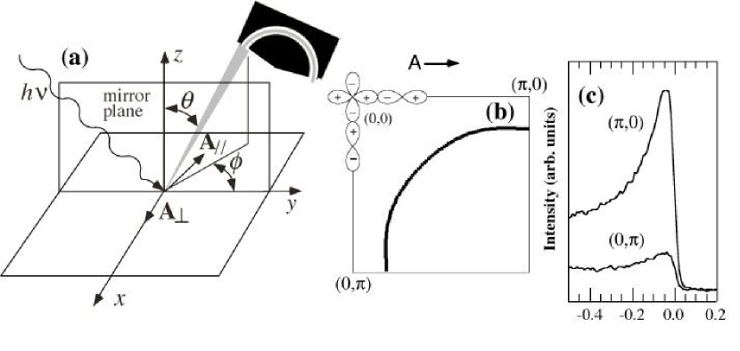
Figure 2: (a) Arrangement of the photon beam and detector in order to make use of the photoemission selection rules. (b) Symmetry of the Cu$3d_{x^{2}-y^{2}}$ orbitals hybridized with the O$2p$ orbitals. (c) EDCs showing the symmetry of the orbitals in (b) obtained at $\hbar\nu=$22 eV.

Let the photon beam be incident along a plane of mirror symmetry of the sample (${\cal M}$), with detector placed in the same mirror plane; see Fig. 2(a). The final state $\psi_{f}$ must then be even with respect to reflection in ${\cal M}$, because if it were odd the wave function would vanish at the detector. (For this discussion it is simpler to imagine changing the photon polarization, keeping the detector fixed. In the actual experiment, however, it is the polarization which is fixed and the detector is moved when checking dipole selection rules.)

The dipole transition is allowed if the entire matrix element has an overall even symmetry. Thus two possibilities arise. (1) For an initial state $\psi_{i}$ which is even with respect to ${\cal M}$, the light polarization ${\bf A}$ must also be even, i.e. parallel to ${\cal M}$. (2) For an initial state odd with respect to ${\cal M}$, ${\bf A}$ must also be odd, i.e. perpendicular to ${\cal M}$. This can be summarized as:

$$\left\langle{\psi_{f}}\right|{\bf A}\cdot\hat{\bf p}\left|{\psi_{i}}\right\rangle\left\{{\matrix{{\psi_{i}\,\,even\,\,\left\langle+\right|+\left|+\right\rangle\,\,\Rightarrow\,\,{\bf A}\,\,even}\cr{\psi_{i}\,\,odd\,\,\left\langle+\right|-\left|-\right\rangle\,\,\Rightarrow\,\,{\bf A}\,\,odd}\cr}}\right.$$ (4)

Consider hybridized $Cu3d-O2p$ initial states, as shown in Fig. 2(b), which have a $d_{x^{2}-y^{2}}$ symmetry about a Cu site. These states are even under reflection in $(0,0)-(\pi,0)$ (i.e. the plane defined by this symmetry axis and the z-axis) and odd with respect to $(0,0)-(\pi,\pi)$. Therefore, measurement along the $(0,0)-(\pi,0)$ direction will be dipole-allowed (forbidden) if the polarization vector A is parallel (perpendicular) to this axis. Fig. 2(c) shows that, consistent with an initial state which is even about $(0,0)-(\pi,0)$, the signal is maximized when ${\bf A}$ lies in the mirror plane and minimized when ${\bf A}$ is perpendicular to this plane. (The reasons for small non-zero intensity in the dipole forbidden geometry are the small, but finite, ${\bf k}$-window of the experiment and the possibility of a small misalignment of the sample). Similarly, we have checked experimentally (for Bi2212 in the Y-quadrant where there are no superlattice complications) that the initial state is consistent with odd symmetry about $(0,0)-(\pi,\pi)$ (see also Ref. SHEN_REVIEW ).

While the dipole matrix elements are strongly photon energy dependent, the selection rules are, of course, independent of photon energy. This has been checked by measurements at 22 eV and 34 eV.mesot01 All of these results are consistent with the fact that we are probing $Cu3d-O2p$ initial one-electron states with $d_{x^{2}-y^{2}}$ symmetry. We will see below that these selection rules are extremely useful in disentangling the main CuO₂ “band” from its umklapp images due to the superlattice in Bi2212.

2.2 The One-Step Model

The three-step model of photoemission gives a very useful zeroth order description of the photoemission process, but it needs to be put on a firmer footing, both as regards the calculation of photoemission intensities from ab-initio electronic structure calculations, and also for developing a deeper understanding of how many-body effects influence ARPES spectra. We now briefly review the so called “one-step” model of photoemission with these goals in mind.

Ever since Hertz and Hallwachs discovered photoemissionHERTZ , it is known that the photo-electron current at the detector is proportional to the incident photon flux, i.e., to the square of the vector potential. Thus photoemission measures a nonlinear response function, and the relevant correlation function is a three current correlator, as first emphasized by Schaich and Ashcroft ASHCROFT . It is instructive to briefly review their argument. As in standard response function calculations, let’s look at an expansion of the current at the detector (the response) in powers of the vector potential of incident photons (the perturbation). Let ${\bf R}$ be the location of the detector in vacuum and ${\bf r}$ denote points inside the sample. The zeroth order contribution $\langle 0|j_{\alpha}({\bf R},t)|0\rangle$ vanishes as there are no currents flowing in the ground state $|0\rangle$ of the unperturbed system. The linear response also vanishes, with $\langle 0|j_{\alpha}({\bf R},t)j_{\beta}({\bf r},t^{\prime})|0\rangle=0$ and $\langle 0|j_{\alpha}({\bf r},t^{\prime})j_{\beta}({\bf R},t)|0\rangle=0$, since there are no particles at the detector, in absence of the electromagnetic field, and $j_{\beta}({\bf R},t)|0\rangle=0$. Thus the leading term which survives is

$$\langle j_{\gamma}({\bf R},t)\rangle\propto\int d{\bf r}^{\prime}dt^{\prime}d{\bf r}^{\prime\prime}dt^{\prime\prime}A_{\alpha}({\bf r}^{\prime},t^{\prime})A_{\beta}({\bf r}^{\prime\prime},t^{\prime\prime})$$ (5)

$$\langle 0|j_{\alpha}({\bf r}^{\prime},t^{\prime})j_{\gamma}({\bf R},t)j_{\beta}({\bf r}^{\prime\prime},t^{\prime\prime})|0\rangle$$ (6)

where only current operators inside the sample act on the unperturbed ground state on either side and the current at the detector is sandwiched in between.

[width=.5]feynman2.epsf

Figure 3: Diagrams contributing to the three-current correlator of ARPES. The physical processes that each diagram represents is discussed in the text.

The three current correlation function can be represented by the triangle diagram shown in Fig. 3(A) CAROLI , where the line between the two external photon vertices is the Greens function of the “initial state” or “photo-hole” and the two lines connecting the photon vertex to the current at the detector represent the “photo-electron” which is emitted from the solid. There is a large literature on the evaluation of the (bare) triangle diagram incorporating the results of ab-initio electronic structure calculations of a semi-infinite solid, including the effects of realistic surface termination and multiple scattering effects in the photo-electron final states. Detailed calculations using this formalism were first carried out by Pendry PENDRY for a system with one atom per unit cell, and later generalized to more complex crystals LARSON ; LINDBERG ; HOPKINSON .

This approach is very reliable for calculating photoemission intensities, and gives important information about “matrix element effects”, i.e., the dependence of the ARPES intensity on ${\bf k}$, and on the incident photon energy and polarization. (It does not, however, shed light on the many-body aspects of the lineshape). Such ab-initio methods have been extensively used by Bansil, Lindroos and coworkers BANSIL for the high $T_{c}$ cuprates.

As an example of the usefulness of ab-initio methods, we show the comparison between the observed and calculated ARPES intensities for YBCO in Fig. 4. Since the calculated intensity is a sensitive function of the termination plane, such a comparison suggests that the crystal breaks at the chains, a conclusion later confirmed by STM measurements DELOZANNE . In fact, it was the complexity of the termination in YBCO, plus the fact that none of the possible cleavage planes of YBCO are charge neutral, and thus involve significant charge transfer, that convinced us to focus primarily on the Bi-based cuprates (Bi2212 and Bi2201). These materials have two adjacent BiO planes which are van der Waals bonded, and thus cleavage leads to neutral surfaces which are not plagued by uncontrolled surface effects. The highly two-dimensional Bi-based cuprates are thus ideal from the point of view of ARPES studies.

[width=1]onestepcomp.epsf

Figure 4: Comparison of the photoemission intensity of states along the zone diagonal in YBCO with (a) even polarization and (b) odd polarization, showing that this state is odd with respect to reflection about the diagonal to the Cu-O bond direction. (c) Comparison of the photoemission intensity to the observed one as a function of polarization. The detailed polarization comparison gives confidence to the interpretation of the observed peak as arising from the Cu-O plane states.

2.3 Single-Particle Spectral Function

Although the one step model gives a reasonable interpretation of the overall intensity in the photoemission process, much of what we really want to learn from the experiment relates to the spectral lineshape, which, as we will show, is strongly influenced by correlations. We must then ask ourselves the important question of how the initial state lineshape enters the ARPES intensity and to what extent this is revealed in the observed lineshape. Although a fully rigorous justification of a simple interpretation of ARPES spectra is not available at the present time, a reasonable case can be made for analyzing the data in terms of the single particle spectral function of the initial state.

We begin by considering the various many body renormalizations of the bare triangle diagram which are shown in Fig. 3. These renormalizations can arise, in principle, from either electron-phonon or electron-electron interactions. These self energy effects and vertex corrections are easy to draw, but impossible to evaluate in any controlled calculation. Nevertheless, they are useful in obtaining a qualitative understanding of the the various processes and estimating their relative importance. Diagram (B) represents the self-energy corrections to the occupied initial state that we are actually interested in studying; (C) and (D) represent final state line-width broadening and inelastic scattering; (E) is a vertex correction that describes the interaction of the escaping photo-electron with the photo-hole in the solid; (F) is a vertex correction which combines features of (D) and (E). (An additional issue in a quantitative theory of photoemission is related to the modification of the external vector potential inside the medium, i.e., renormalizations of the photon line. These are considered in detail in Ref. BANSIL ).

If the sudden approximation is valid, we can neglect the vertex corrections: the outgoing photo-electron is moving so fast that it has no time to interact with the photo-hole. Let us make simple time scale estimates for the cuprates with 15 - 30 eV (ultraviolet) incident photons. The time $t$ spent by the escaping photo-electron in the vicinity of the photo-hole is the time available for their interaction. A photoelectron with a kinetic energy of (say) 20 eV has a velocity $v=3\times 10^{8}$ cm/s. The relevant length scale, which is the smaller of the screening radius (of the photo-hole) and the escape depth, is $\sim 10\AA$. Thus $t=3\times 10^{-16}$ s, which should be compared with the time scale for electron-electron interactions (which are the dominant source of interactions at the high energies of interest): $t_{ee}=(2\pi)/\omega_{p}=4\times 10^{-15}$ s, using a plasma frequency $\omega_{p}=1$ eV for the cuprates (this would be even slower if c-axis plasmons are involved). If $t\ll t_{ee}$, then we can safely ignore vertex corrections. From our very crude estimate $t/t_{ee}=0.1$, so that the situation with regard to the validity of the impulse approximation is not hopeless, but clearly, experimental checks are needed, and we present these in the next subsection.

Very similar estimates can be made for renormalizations of the outgoing photo-electron due to its interaction with the medium; again electron-electron interactions dominate at the energies of interest. The relevant length scale here is the escape depth, which leads to a process of self-selection: those electrons that actually make it to the detector with an appreciable kinetic energy have suffered no collisions in the medium. Such estimates indicate that the “inelastic background” must be small and we will show how to experimentally obtain its precise dependence on ${\bf k}$ and $\omega$ later.

Finally, one expects that final state linewidth corrections are small for quasi-2D materials based on the estimates made by Smith et al. SMITH In fact, this is yet another reason for the ease of interpreting ARPES data in quasi-2D materials. A clear experimental proof that these effects are negligible for Bi2212 will be presented later, where it will be seen that deep in the superconducting state, a resolution limited leading edge is obtained for the quasiparticle peak.

2.4 Spectral Functions and Sum Rules

Based on the arguments presented in the preceding subsection, we assume the validity of the sudden approximation and ignore both the final-state linewidth broadening and the additive extrinsic background. Then (B) is the only term that survives from all the terms described in Fig. 3 and the ARPES intensity is given by hedin ; NK

$$I({\bf k},\omega)=I_{0}({\bf k})f(\omega)A({\bf k},\omega)$$ (7)

where ${\bf k}$ is the initial state momentum in the 2D Brillouin zone and $\omega$ the energy relative to the chemical potential. The prefactor $I_{0}({\bf k})$ includes all the kinematical factors and the square of the dipole matrix element (shown in Eq. 3), $f(\omega)$ is the Fermi function, and $A({\bf k},\omega)$ is the one-particle spectral function which will be described in detail below.

We first describe some general consequences of Eq. 7 based on sum rules and their experimental checks. The success of this strategy employed by Randeria et al. NK greatly strengthens the case for a simple $A({\bf k},\omega)$ interpretation of ARPES data.

The one-particle spectral function represents the probability of adding or removing a particle from the interacting many-body system, and is defined as $A({\bf k},\omega)=-(1/\pi){\rm Im}G({\bf k},\omega+i0^{+})$ in terms of the Green’s function. It can be written as the sum of two pieces $A({\bf k},\omega)=A_{-}({\bf k},\omega)+A_{+}({\bf k},\omega)$, where the spectral weight to add an electron to the system is given by $A_{+}({\bf k},\omega)=Z^{-1}\sum_{m,n}e^{-\beta{\cal E}_{m}}|\langle n|c^{\dagger}_{\bf k}|m\rangle|^{2}\delta(\omega+{\cal E}_{m}-{\cal E}_{n})$, and that to extract an electron is $A_{-}({\bf k},\omega)=Z^{-1}\sum_{m,n}e^{-\beta{\cal E}_{m}}|\langle n|c_{\bf k}|m\rangle|^{2}\delta(\omega+{\cal E}_{n}-{\cal E}_{m})$. Here $|m\rangle$ is an exact eigenstate of the many-body system with energy ${\cal E}_{m}$, $Z$ is the partition function and $\beta=1/T$. It follows from these definitions that $A_{-}({\bf k},\omega)=f(\omega)A({\bf k},\omega)$ and $A_{+}({\bf k},\omega)=\left[1-f(\omega)\right]A({\bf k},\omega)$, where $f(\omega)=1/[\exp(\beta\omega)+1]$ is the Fermi function. Since an ARPES experiment involves removing an electron from the system, the simple golden rule Eq. 3 can be generalized to yield an intensity proportional to $A_{-}({\bf k},\omega)$

We now discuss various sum rules for $A({\bf k},\omega)$ and their possible relevance to ARPES intensity $I({\bf k},\omega)$. While the prefactor $I_{0}$ depends on ${\bf k}$ and also on the incident photon energy and polarization, it does not have any significant $\omega$ or $T$ dependence. Thus the energy dependence of the ARPES lineshape and its $T$ dependence are completely characterized by the spectral function and the Fermi factor. The simplest sum rule $\int_{-\infty}^{+\infty}d\omega A({\bf k},\omega)=1$ is not useful for ARPES since it involves both occupied (through $A_{-}$) and unoccupied states ($A_{+}$). Next, the density of states (DOS) sum rule $\sum_{\bf k}A({\bf k},\omega)=N(\omega)$ is also not directly useful since the prefactor $I_{0}$ has very strong ${\bf k}$-dependence. However it may be useful to ${\bf k}$-sum ARPES data $N_{p}(\omega)=\sum_{\bf k}I_{0}({\bf k})A({\bf k},\omega)$ in an attempt to simulate the angle-integrated photoemission intensity.

The important sum rule for ARPES is

$$\int_{-\infty}^{+\infty}d\omega f(\omega)A({\bf k},\omega)=n({\bf k}),$$ (8)

which directly relates the energy-integrated ARPES intensity to the momentum distribution $n({\bf k})=\langle c^{\dagger}_{\bf k}c_{\bf k}\rangle$. (The sum over spins is omitted for simplicity). Somewhat surprisingly, the usefulness of this sum rule has been overlooked in the ARPES literature prior to Ref. NK .

We first focus on the Fermi surface ${\bf k}={\bf k}_{F}$. One of the major issues, that we will return to several times in the remainder of this article, will be the question of how to define “${\bf k}_{F}$” at finite temperatures in a strongly correlated system which may not even have well-defined quasiparticle excitations, and how to determine it experimentally. For now, we simply define the Fermi surface to be the locus of gapless excitations in ${\bf k}$-space in the normal state, so that $A({\bf k}_{F},\omega)$ has a peak at $\omega=0$.

To make further progress with Eq. (8), we need to make a weak particle-hole symmetry assumption: $A({\bf k}_{F},-\omega)=A({\bf k}_{F},\omega)$ for “small” $\omega$, where “small” means those frequencies for which there is significant $T$-dependence in the spectral function. It then follows that NK $\partial n({\bf k}_{F})/\partial T=0$, i.e., the integrated area under the EDC at ${\bf k}_{F}$ is independent of temperature. To see this, rewrite Eq. (8) as $n({\bf k}_{F})={1\over 2}-{1\over 2}\int_{0}^{\infty}d\omega\tanh\left(\omega/2T\right)\left[A({\bf k}_{F},\omega)-A({\bf k}_{F},-\omega)\right]$, and take its $T$-derivative. It should be emphasized that we cannot say anything about the value of $n({\bf k}_{F})$, only that it is $T$-independent. (A much stronger assumption, $A({\bf k}_{F},-\omega)=A({\bf k}_{F},\omega)$ for all $\omega$, is sufficient to give $n({\bf k}_{F})=1/2$ independent of $T$). We emphasize the approximate nature of the ${\bf k}_{F}$-sum-rule since there is no exact symmetry that enforces it.

We note that we did not make use of any properties of the spectral function other than the weak particle-hole symmetry assumption, and to the extent that this is also valid in the superconducting state, our conclusion $\partial n({\bf k}_{F})/\partial T=0$ holds equally well below $T_{c}$. There is the subtle issue of the meaning of “${\bf k}_{F}$” in the superconducting state. In analogy with the Fermi surface as the “locus of gapless excitations” above $T_{c}$, we can define the “minimum gap locus” below $T_{c}$. We will describe this in great detail in Sect. 5.1 below; it suffices to note here that “${\bf k}_{F}$” is independent of temperature, within experimental errors, in both the normal and superconducting states of the systems studied thus far DING95 .

[width=.5]edcvstatef.epsf

Figure 5: (a) ARPES spectra for Bi2212 at the ${\bf k}_{F}$ point shown in the zone inset in the normal and superconducting states. (b) Integrated intensity as a function of temperature at the same $k$ point.

In Fig. 5(a) we show ARPES spectra for near-optimal Bi2212 ($T_{c}=87$ K) at ${\bf k}_{F}$ along $(\pi,0)$ to $(\pi,\pi)$ at two temperatures: $T=13$ K, which is well below $T_{c}$, and $T=95$ K, which is in the normal state. The two data sets were normalized in the positive energy region, which after normalization was chosen to be the common zero baseline. (The essentially $\omega$-independent emission at positive energies, which is not cut-off by the Fermi function, is due to higher harmonics of the incident photon beam, called “second order light”). For details, see Ref. NK .

In Fig. 5(b) we plot the integrated intensity as a function of $T$ and find that, in spite of the remarkable changes in the lineshape from 95K to 13K, the integrated intensity at ${\bf k}_{F}$ is very weakly $T$-dependent, verifying the sum rule $\partial n({\bf k}_{F})/\partial T=0$. The error bars come from the normalization due to the low count rate in the $\omega>0$ background.

Let us discuss several other potential complications in testing the $T$-independence of the integrated intensity at ${\bf k}_{F}$. Note that matrix elements have no effect on this result, since they are $T$-independent. The same is true for a $T$-independent additive extrinsic background. In an actual experiment the observed intensity will involve convolution of Eq. 7 with the energy resolution and a sum over the ${\bf k}$-values within the momentum window. While energy resolution is irrelevant to an integrated quantity, sharp ${\bf k}$-resolution is of the essence.

The $T$-independence of the integrated intensity is insensitive to the choice of the integration cutoff at negative $\omega$, provided it is chosen beyond the dip feature. It has been observed experimentally that the normalized EDCs at ${\bf k}_{F}$ have identical intensities for all $\omega<-100$meV. This is quite reasonable, since we expect the spectral functions to be the same for energies much larger than the scale associated with superconductivity. The fact that one has to go to 100meV (much larger than $T_{c}\sim 10meV$) in order to satisfy the sum rule suggests that electron-electron interactions are involved in superconductivity.

2.5 Analysis of ARPES Spectra: EDCs and MDCs

In the preceding subsections we have presented evidence in favor of a simple spectral function interpretation of ARPES data on the quasi 2D high $T_{c}$ cuprates. In the process, we saw that the ARPES intensity in Fig. 5 has a nontrivial lineshape which has a significant temperature dependence. We now introduce some of the basic ideas which will be used throughout the rest of the article to analyze and understand the ARPES lineshape.

The one-electron Green’s function can be generally written as $G^{-1}({\bf k},\omega)=G_{0}^{-1}({\bf k},\omega)-\Sigma({\bf k},\omega)$ where $G_{0}({\bf k},\omega)=1/[\omega-\varepsilon_{\bf k}]$ is the Green’s function of the noninteracting system, $\varepsilon_{\bf k}$ is the “bare” dispersion, and the (complex) self-energy $\Sigma({\bf k},\omega)=\Sigma^{\prime}({\bf k},\omega)+i\Sigma^{\prime\prime}({\bf k},\omega)$ encapsulates the effects of all the many-body interactions. Then using its definition in terms of ${\rm Im}G$, we obtain the general result

$$A({\bf k},\omega)={1\over\pi}{{\Sigma^{\prime\prime}({\bf k},\omega)}\over{\left[{\omega-\varepsilon_{\bf k}-\Sigma^{\prime}({\bf k},\omega)}\right]^{2}+\left[{\Sigma^{\prime\prime}({\bf k},\omega)}\right]^{2}}}$$ (9)

We emphasize that this expression is entirely general, and does not make any assumptions about the validity of perturbation theory or of Fermi liquid theory.

New electron energy analyzers, which measure the photoemitted intensity as a function of energy and momentum simultaneously, allow the direct visualization of the spectral function, as shown in Fig. 6, and have also suggested new ways of plotting and analyzing ARPES data. (a) In the traditional energy distribution curves (EDCs), the measured intensity $I({\bf k},\omega)$ is plotted as a function of $\omega$ (binding energy) for a fixed value of ${\bf k}$; and (b) In the new Valla99 momentum distribution curves (MDCs), $I({\bf k},\omega)$ is plotted at fixed $\omega$ as a function of ${\bf k}$.

[width=.5]spectralfn.epsf

Figure 6: (a) The ARPES intensity as a function of ${\bf k}$ and $\omega$ at $h\nu$=22eV and T=40K. main is the main band, and SL a superlattice image. (b) A constant $\omega$ cut (MDC) from (a). (c) A constant ${\bf k}$ cut (EDC) from (a). The diagonal line in the zone inset shows the location of the ${\bf k}$ cut; the curved line is the Fermi surface.

Until a few years ago, the only data available were in the form of EDCs, and even today this is the most useful way to analyze data corresponding to gapped states (superconducting and pseudogap phases). These analyses will be discussed in great detail in subsequent sections. We note here some of the issues in analyzing EDCs and then contrast them with the MDCs. First, note that the EDC lineshape is non-Lorentzian as a function of $\omega$ for two reasons. The trivial reason is the asymmetry introduced by the Fermi function $f(\omega)$ which chops off the positive $\omega$ part of the spectral function. (We will discuss later on ways of eliminating the effect of the Fermi function). The more significant reason is that the self energy has non-trivial $\omega$ dependence and this makes even the full $A({\bf k},\omega)$ non-Lorentzian in $\omega$ as seen from Eq. 9. Thus one is usually forced to model the self energy and make fits to the EDCs. At this point one is further hampered by the lack of detailed knowledge of the additive extrinsic background which itself has $\omega$-dependence. (Although, as we shall see, the MDC analysis give a new way of determining this background).

The MDCs obtained from the new analyzers have certain advantages in studying gapless excitations near the Fermi surface Valla99 ; Kink ; Adam01 . In an MDC the intensity is plotted as a function of $k$ varying normal to the Fermi surface in the vicinity of a fixed ${\bf k}_{F}(\theta)$, where $\theta$ is the angle parametrizing the Fermi surface. For $k$ near $k_{F}$ we may linearize the bare dispersion $\varepsilon_{\bf k}\simeq v_{F}^{0}(k-k_{F})$, where $v_{F}^{0}(\theta)$ is the bare Fermi velocity. We will not explicitly show the $\theta$ dependences of $k_{F}$, $v_{F}^{0}$, or other quantities considered below, in order to simplify the notation.

Next we make certain simplifying assumptions about the remaining ${\bf k}$-dependences in the intensity $I({\bf k},\omega)$. We assume that: (i) the self-energy $\Sigma$ is essentially independent of $k$ normal to the Fermi surface, but can have arbitrary dependence on $\theta$ along the Fermi surface; and (ii) the prefactor $I_{0}({\bf k})$ does not have significant $k$ dependence over the range of interest. It is then easy to see from Eqs. 7 and 9 that $I({\bf k},\omega)$ plotted as function $k$ (with fixed $\omega$ and $\theta$) has the following lineshape. The MDC is a Lorentzian: (a) centered at $k=k_{F}+[\omega-\Sigma^{\prime}(\omega)]/v_{F}^{0}$; with (b) width (HWHM) $W_{M}=|\Sigma^{\prime\prime}(\omega)|/v_{F}^{0}$.

Thus the MDC has a very simple lineshape, and its peak position gives the renormalized dispersion, while its width is proportional to the imaginary self energy. The consistency of the assumptions made in reaching this conclusion may be tested by simply checking whether the MDC lineshape is fit by a Lorentzian or not. Experimentally, excellent Lorentzian fits are invariably obtained (except when one is very near the bottom of the “band” or in a gapped stateMDC01 ).

Finally, note that the external background in the case of MDCs is also very simple. One can fit the MDC (at each $\omega$) to a Lorentzian plus a constant (at worst Lorentzian plus linear in $k$) background. From this one obtains the value of the external background including its $\omega$ dependence. Now this $\omega$-dependent background can be subtracted off from the EDC also, if one wishes to. Note that estimating this background was not possible from an analysis of the EDCs alone.

3 The Valence Band

The basic unit common to all cuprates is the copper-oxide plane, $CuO_{2}$. Some compounds have a tetragonal cell, $a=b$, such as the $Tl$ compounds, but most have an orthorhombic cell, with $a$ and $b$ differing by as much as 3% in YBCO. There are two notations used in the literature for the reciprocal cell. The one used here, appropriate for Bi2212 and Bi2201, has $\Gamma-M$ along the $Cu-O$ bond direction, with $M\equiv(\pi,0)$, and $\Gamma-X(Y)$ along the diagonal, with $Y\equiv(\pi,\pi)$. The other notation, appropriate to YBCO, has $\Gamma-X(Y)$ along the $Cu-O$ bond direction and $\Gamma-S$ along the diagonal. This difference occurs because the orthorhombic distortion in one compound is rotated $45^{\circ}$ with respect to the other. The main effect of the orthorhombicity in Bi2212 and Bi2201 is the superlattice modulation along the $b$ axis, with $Q_{SL}$ parallel to $\Gamma-Y$. Except when refering to this modulation, we will assume tetragonal symmetry in our discussions. For a complete review of the electronic structure of the cuprates, see Ref. PICKETT .

The Cu ions are four fold coordinated to planar oxygens. Apical (out of plane oxygens) exist in some structures (LSCO), but not in others. Either way, the apical bond distance is considerably longer than the planar one, so in all cases, the cubic point group symmetry of the Cu ions is lowered, leading to the highest energy Cu state having $d_{x^{2}-y^{2}}$ symmetry. As the atomic $3d$ and $2p$ states are nearly degenerate, a characteristic which distinguishes cuprates from other 3d transition metal oxides, the net result is a strong bonding-antibonding splitting of the Cu $3d_{x^{2}-y^{2}}$ and O $2p$ $\sigma$ states, with all other states lying in between. In the stochiometric (undoped) material, Cu is in a $d^{9}$ configuration, leading to the upper (antibonding) state being half filled. According to band theory, the system should be a metal. But in the undoped case, integer occupation of atomic orbitals is possible, and correlations due to the strong on-site Coulomb repulsion on the Cu sites leads to an insulating state. That is, the antibonding band “Mott-Hubbardizes” and splits into two, one completely filled (lower Hubbard band), the other completely empty (upper Hubbard band) PHIL .

On the other hand, for dopings characteristic of the superconducting state, a large Fermi surface is observed by ARPES (as discussed in the next section). Thus, to a first approximation, the basic electronic structure in this doping range can be understood from simple band theory considerations. The simplest approximation is to consider the single Cu $3d_{x^{2}-y^{2}}$ and two O $2p$ (x,y) orbitals. The resulting secular equation is OKA

$$\left(\begin{array}[]{ccc}\epsilon_{d}&2t\sin(k_{x}a)&-2t\sin(k_{y}a)\\ 2t\sin(k_{x}a)&\epsilon_{p}&0\\ -2t\sin(k_{y}a)&0&\epsilon_{p}\end{array}\right)$$ (13)

where $\epsilon_{d}$ is the atomic $3d$ orbital energy, $\epsilon_{p}$ is the atomic $2p$ orbital energy, and $t$ is the Cu-O hopping integral. Diagonalization of this equation leads to a non-bonding eigenvalue $E_{nb}=\epsilon_{p}$, and

$$E_{\pm}=\frac{\epsilon_{p}+\epsilon_{d}}{2}\pm\sqrt{(\frac{\epsilon_{p}-\epsilon_{d}}{2})^{2}+4t^{2}(\sin^{2}(k_{x}a)+\sin^{2}(k_{y}a))}$$ (14)

where + refers to antibonding, - to bonding. This dispersion is shown in Fig. 7(a)

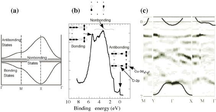
Figure 7: (a) Simple three band estimate of the electronic structure of the Cu-O plane states; (b) EDC showing the whole valence band at the ($\pi,0$) point; c) Intensity map of the whole valence band obtained by taking the second derivative of spectra such as the one in (b). The orbitals in (b) are based on the three band model, where black and white lobes corresponding to positive and negative wavefunctions.

In Fig. 7(b), we show an ARPES spectrum obtained at the $(\pi,0)$ point of the Brillouin zone for Bi2212. Three distinct features can be observed: the bonding state at roughly -6eV, the antibonding state near the Fermi energy, and the rest of the states in between. This rest consists of the non-bonding state mentioned above, as well as the remainder of the Cu $3d$ and O $2p$ orbitals, plus states originating from the other (non Cu-O) planes. It is difficult to identify all of these “non-bonding” states, as their close proximity and broadness causes them to overlap in energy. Perhaps surprisingly, the overall picture of the electronic structure of the valence band has the structure that one would predict by the simple chemical arguments given above, as shown in Fig. 7(c). The most important conclusion that one can derive from Fig 7 is the early prediction by Anderson RVB0 , namely that there is a single state relevant to transport and superconducting properties. This state, the antibonding state in Fig 7, is well separated from the rest of the states, and therefore any reasonable theoretical description of the physical properties of these novel materials should arise from this single state.

Despite these simple considerations, correlation effects do play a major role, even in the doped state. The observed antibonding band width is about a factor of 2-3 narrower than that predicted by band theory OLSON . In fact, the correlation effects are the ones we are most interested in, as they give rise to the many unusual properties of the cuprates, including the superconducting state.

As mentioned above, in the magnetic insulating regime, the picture is quite different. The antibonding band splits into two, with the chemical potential lying in the gap WELLS . Upon doping with electrons or holes, the chemical potential would move up or down. One would then expect to observe small Fermi surfaces, hole pockets centered at $(\pi/2,\pi/2)$ with a volume equal to the hole doping, $x$. These can be generated at the mean field level by folding Fig. 7(a) back into the magnetic zone with Q=$(\pi,\pi)$, and turning on an interaction, $U_{eff}$, between the two folded bands. This can be contrasted with the large Fermi surface of the unfolded case, typically centered at $(\pi,\pi)$ with a volume $1+x$. It is still an open question whether there is a continuous evolution between these two limits, or whether there is a discontinuous change at a metal-insulator transition point. In any case, a proper description of the electronic structure must take the strong electron-electron correlations into account, even in the superconducting regime.

4 Normal State Dispersion and the Fermi Surface

The Fermi surface is one of the central concepts in the theory of metals, with electronic excitations near the Fermi surface dominating all the low energy properties of the system. In this Section we describe the use of ARPES to elucidate the electronic structure and the Fermi surface of the high $T_{c}$ superconductors.

It is important to discuss these results in detail because ARPES is the only experimental probe which has yielded useful information about the electronic structure and the Fermi surface of the planar Cu-O states which are important for high $T_{c}$ superconductivity. Traditional tools for studying the Fermi surface such as the deHaas-van Alphen effect have not yielded useful information about the cuprates, because of the need for very high magnetic fields, and possibly because of the lack of well defined quasiparticles. Other Fermi surface probes like positron annihilation are hampered by the fact that the positrons appear to preferentially probe spatial regions other than the Cu-O planes.

The first issue facing us is: what do we mean by a Fermi surface in a system at high temperatures where there are no well-defined quasiparticles? (Recall that quasiparticles, if they exist, manifest themselves as sharp peaks in the one-electron spectral function whose width is less than their energy, and lead to a jump discontinuity in the momentum distribution at $T=0$.) Clearly, the traditional $T=0$ definition of a Fermi surface defined by the jump discontinuity in $n({\bf k})$ is not useful for the cuprates. First, the systems of interest are superconducting at low temperatures. But even samples which have low $T_{c}$’s have normal state peak widths at $E_{f}$ which are an order of magnitude broader than the temperatureAdam00 ; Adam01 . If, as indicated both by ARPES and transport, sharp quasiparticle excitations do not exist above $T_{c}$, there is no possibility of observing a thermally-smeared, resolution-broadened, discontinuity in $n({\bf k})$.

It is an experimental fact that in the cuprates ARPES sees broad peaks which disperse as a function of momentum and go through the chemical potential at a reasonably well-defined momentum. We can thus adopt a practical definition of the “Fermi surface” in these materials as “the locus of gapless excitations”.

Historically, the first attempts to determine the Fermi surface in cuprates were made on YBCOCAMPUZANO_90 , however, surface effects as well as the presence of chains appear to complicate the picture, so we will focus principally on Bi2212 and Bi2201, which have been studied the most intensively. Other cuprates which have also been studied by ARPES, include the electron-doped material NCCO NCCO and, more recently, LSCO as a function of hole doping LSCO .

We discuss below various methods used for the determination of the spectral function peaks in the vicinity of $E_{f}$. In addition, we supplement these methods with momentum distribution studies, taking due care of matrix element complications. We will then discuss three topics: the extended saddle-point in the dispersion, the search for bilayer splitting in Bi2212, and (in Section 6.4) the doping dependence of the Fermi surface.

4.1 Normal State Dispersion in Bi2212: A First Look

We begin with the results obtained by using the traditional method of deducing the dispersion and Fermi surface by studying the EDC peaks as a function of momentum. This method was used for the cuprates by Campuzano et al.CAMPUZANO_90 , Olson et al.OLSON , and Shen and Dessau SHEN_REVIEW , culminating in the very detailed study of Ding et al.DING_96 . The use of EDC peak dispersion has some limitations which we discuss below. Nevertheless, it has led to very considerable understanding of the overall electronic structure, Fermi surface, and of superlattice effects in Bi2212, and therefore it is worthwhile to review its results first, before turning to more refined methods.

The main results of Ding et al.DING_96 on the electronic dispersion and the Fermi surface in the normal state ($T=95$K) of near-optimal OD Bi2212 ($T_{c}=87$K) using incident photon energies of 19 and 22 eV are summarized in Fig. 8. The peak positions of the EDC’s as a function of ${\bf k}$ are marked with various symbols in Fig. 8(b). The filled circles are for odd initial states (relative to the corresponding mirror plane), open circles for even initial states, and triangles for data taken in a mixed geometry (i.e. the photon polarization was at $45^{\circ}$ to the mirror plane). The Fermi surface crossings corresponding to these dispersing states are estimated from the ${\bf k}$-point at which the EDC peak positions go through the chemical potential when extrapolated from the occupied side. The $k_{F}$ estimates are plotted as open symbols in Fig. 8(a).

We use the following square lattice notation for the 2D Brillouin zone of Bi2212: $\Gamma{\bar{M}}$ is along the CuO bond direction, with $\Gamma=(0,0)$, ${\bar{M}}=(\pi,0)$, $X=(\pi,-\pi)$ and $Y=(\pi,\pi)$ in units of $1/a^{*}$, where $a^{*}=3.83\AA$ is the separation between near-neighbor planar Cu ions. (The orthorhombic a axis is along $X$ and b axis along $Y$).

[width=.5]ns1.epsf

Figure 8: Fermi surface (a) and dispersion (b) obtained from normal state measurements. The thick lines are obtained by a tight binding fit to the dispersion data of the main band with the thin lines $(0.21\pi,0.21\pi)$ umklapps and the dashed lines $(\pi,\pi)$ umklapps of the main band. Open circles in (a) are the data. In (b), filled circles are for odd initial states (relative to the corresponding mirror plane), open circles for even initial states, and triangles for data taken in a mixed geometry. The inset of (b) is a blowup of $\Gamma X$.

In addition to the symbols obtained from data in Fig. 8, there are also several curves which clarify the significance of all of the observed features. The thick curve in Fig. 8(b) is $\epsilon({\bf k})$, a six-parameter tight-binding fit NORMAN_95a to the dispersion data in the $Y$-quadrant; this represents the main CuO₂ “band”. It cannot be overemphasized that, although this dispersion looks very much like band theory (except for an overall renormalization of the bandwidth by a factor of 2 to 3), the actual normal state lineshape is highly anomalous. As discussed in Section 7 below, there are no well defined quasiparticles in the normal state.

The thin curves in Fig. 8(b) are $\epsilon({\bf k}\pm{\bf Q})$, obtained by shifting the main band fit by $\pm{\bf Q}$ respectively, where ${\bf Q}=(0.21\pi,0.21\pi)$ is the superlattice (SL) vector known from structural studies SUPERLATTICE . We also have a few data points lying on a dashed curve $\epsilon({\bf k}+{\bf K}_{\pi})$ with ${\bf K}_{\pi}=(\pi,\pi)$; this is the “shadow band” discussed below.

The thick curve in Fig. 8(a) is the Fermi surface contour obtained from the main band fit, while the Fermi surfaces corresponding to the SL bands are the thin lines and that for the shadow band is dashed. It is very important to note that the shifted dispersion curves and Fermi surfaces provide an excellent description of the data points that do not lie on main band. We note that the main Fermi surface is a large hole-like barrel centered about the $(\pi,\pi)$ point whose enclosed area corresponds to approximately 0.17 holes per planar Cu. One of the key questions is why only one CuO main band is found in Bi2212 which is a bilayer material with two CuO planes per unit cell. We postpone discussion of this important issue to end of this Section.

The “shadow bands” seen above, were first observed by Aebi et al. AEBI in ARPES experiments done in a mode similar to the MDCs by measuring as a function of ${\bf k}$ the intensity $\int_{\delta\omega}d\omega f(\omega)A({\bf k},\omega)$ integrated over a small range $\delta\omega$ near $\omega=0$. The physical origin of these “shadow bands” is not certain at the present time. They were predicted early on to arise from short ranged antiferromagnetic correlations KAMPF . In this case the effect should become stronger with underdoping toward the AFM insulator, for which there is little experimental evidence DING_97 . An alternative explanation is that the shadow bands are of structural origin: Bi2212 has a face-centered orthorhombic cell with two inequivalent Cu sites per plane, which by itself could generate a $(\pi,\pi)$ foldback. Interestingly, it has been recently observed that the shadow band intensity is maximal at optimal doping KORDYUK .

We now turn to the effect of the superlattice (SL) on the ARPES spectra. This is very important, since a lack of understanding of these effects has led to much confusion regarding such basic issues as the Fermi surface topology (see below), and the anisotropy of the SC gap (see Section 5). The data strongly suggest BIO_SL that these “SL bands” arise due to diffraction of the outgoing photoelectron off the structural superlattice distortion (which lives primarily) on the Bi-O layer, thus leading to “ghost” images of the electronic structure at $\epsilon_{\bf k\pm Q}$.

We emphasize the use of polarization selection rules (discussed in Section 2.1) for ascertaining various important points. First, we use them to carefully check the absence of a Fermi crossing for the main band along $(0,0)-(\pi,0)$, i.e. $\Gamma\bar{M}$. Note that the Fermi crossing that we do see near $(\pi,0)$ along $\Gamma\bar{M}$ in Fig. 8(a) is clearly associated with a superlattice umklapp band, as seen both from the dispersion data in Fig. 8(b) and its polarization analysis. This Fermi crossing is only seen in the $\Gamma\bar{M}\perp$ (odd) geometry both in our data and in earlier work DESSAU_93 . Emission from the main $d_{x^{2}-y^{2}}$ band, which is even about $\Gamma\bar{M}$, is dipole forbidden, and one only observes a weak superlattice signal crossing $E_{f}$. (We will return below to newer data at different incident photon energies where the possibility of a Fermi crossing along $\Gamma\bar{M}$ is raised again).

Second, we use polarization selection rules to disentangle the main and SL bands in the $X$-quadrant where the main and umklapp Fermi surfaces are very close together; see Fig. 8(a). The point is that $\Gamma X$ (together with the $z$-axis) and, similarly $\Gamma Y$, are mirror planes, and an initial state arising from an orbital which has $d_{x^{2}-y^{2}}$ symmetry about a planar Cu-site is odd under reflection in these mirror planes. With the detector placed in the mirror plane the final state is even, and one expects a dipole-allowed transition when the photon polarization ${\bf A}$ is perpendicular to (odd about) the mirror plane, but no emission when the polarization is parallel to (even about) the mirror plane. While this selection rule is obeyed along $\Gamma Y$ it is violated along $\Gamma X$. In fact this apparent violation of selection rules in the X quadrant was a puzzling feature of all previous studies SHEN_REVIEW of Bi2212. It was first pointed out in Ref. NORMAN_95b , and then experimentally verified in Ref. DING_96 , that this “forbidden” $\Gamma X||$ emission originates from the SL umklapps. We will come back to the $\Gamma X||$ emission in the superconducting state below.

4.2 Improved Methods for Fermi Surface Determination

We now discuss more recently developed methodologies for Fermi surface determination. The need for these improvements arises in part from the practical difficulty of determining precisely where in ${\bf k}$-space a state goes through $E_{f}$. This problem is particularly severe in the vicinity of the $(\pi,0)$ point of the zone where one is beset by the following complications in both Bi2201 and 2212: (1) The normal state ARPES peaks are very broad. This has important implications about the (non-Fermi-liquid) nature of the the normal state, as discussed later (section 7). (2) The electronic dispersion near $(\pi,0)$ is anomalously flat (“extended saddle-point”). (3) In Bi2212 the superlattice structure complicates the interpretation of the data as described above. Fortunately this complication is greatly reduced in Pb-doped Bi2201 and 2212. (4) The final complication comes from the strong variation of the ${\bf k}$-dependent ARPES matrix elements with incident photon energy. This makes the use of changes in absolute intensity as a function of ${\bf k}$ to estimate Fermi surface crossings highly questionable.

Note that the first two points are intrinsic problems intimately related to the physics of high $T_{c}$ superconductivity, the third is a material-specific problem, while the last is specific to the technique of ARPES. Nevertheless, all of these issues must be dealt with adequately before ARPES data on Bi2212 can be used to yield definitive results on the Fermi surface.

Eliminating the Fermi function: Recall that the peak of the EDC as a function of $\omega$ corresponds to that of $f(\omega)A({\bf k},\omega)$, which in general does not coincide with the peak of the spectral function $A({\bf k},\omega)$. If one has a broad spectral function, which at $k_{F}$ is centered about $\omega=0$, then the peak of the EDC will be at $\omega<0$ (positive binding energy), produced by the Fermi function $f(\omega)$ chopping off the peak of $A$, in addition to resolution effects.

Since the goal is to study the dispersive peaks in $A({\bf k},\omega)$, rather than in the EDC, one must effectively eliminate the Fermi function from the observed intensity. We present two ways of achieving this goal, and illustrate it with data on Bi2201 where it permits us to study the broad and weakly dispersive spectral peaks (points (1) and (2) above) near $(\pi,0)$ without the additional complication of the superlattice.

One approach is simply to divide the data by the Fermi function; more accurately one divides the measured intensity $I(\textbf{k}_{F},\omega)$ by $f(\omega)\ast R(\omega)$, the convolution of the Fermi function with the energy resolution. Although this does not rigorously give the spectral function (because of the convolution), this is a good approximation in situations where the energy resolution is very sharp. An excellent example of such an approach can be seen in the work of Sato et al.sato01 on Pb-doped Bi2201 (Bi_1.80Pb_0.38Sr_2.01CuO_6-δ) which is overdoped with a $T_{c}<4K$. In Fig. 4.2 we show the raw data in the vicinity of $M$ at various temperatures in the left panel and the corresponding data “divided by the Fermi function” in the right panel. The “divided” data permits one to clearly observe the dispersion well above $E_{f}$ particularly at high temperatures, and thereby identify the Fermi crossings with a great degree of confidence.

Left panel: temperature dependence of ARPES intensity of OD Bi2201 ($T_{c}<4K$) along the $(\pi,0)-(\pi,\pi)$ cut. Right panel: same divided by the Fermi function at each temperature convoluted with a Gaussian of width 11 meV (energy resolution). Dotted lines show the energy above $E_{f}$ at which the Fermi function takes a value of 0.03. The solid line in the 140 K data indicates the peak positions obtained by fitting with a Lorentzian.

An alternative approach mesot01 to eliminating the Fermi function is to symmetrize the data. For each ${\bf k}$ define the symmetrized intensity by $I_{\rm sym}(\textbf{k}_{F},\omega)=I(\textbf{k}_{F},\omega)+I(\textbf{k}_{F},-\omega)=I_{0}\,A_{sym}(\textbf{k}_{F},\omega)$. It is easy to show that $I_{\rm sym}(\omega)$ will exhibit a local minimum, or dip, at $\omega=0$ for an occupied ${\bf k}$ state, while it will show a local maximum at $\omega=0$ for an unoccupied ${\bf k}$ state. In practice, then, the Fermi crossing ${\bf k}_{F}$ is determined as follows: All EDCs along a cut are symmetrized and ${\bf k}_{F}$ is identified as the boundary in ${\bf k}$-space between points where $I_{\rm sym}$ has a local maximum versus a local minimum at $\omega=0$. As shown in Ref. mesot01 , these arguments work even in the presence of finite resolution effects. We note that this method, and the one presented above, for eliminating the Fermi function require a very accurate determination of the chemical potential (zero of binding energy).

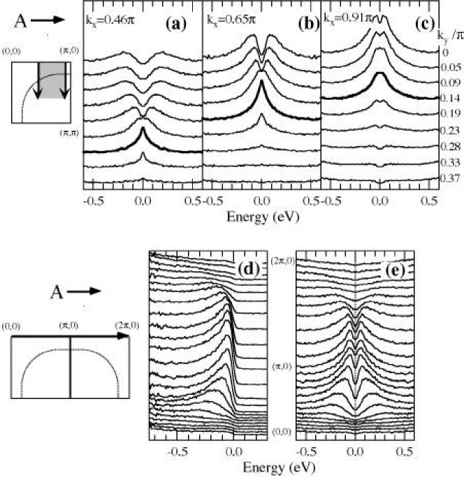
Figure 9: (a,b,c) Symmetrized EDCs along cuts parallel to $(\pi,0)$ to $(\pi,\pi)$ for OD 23K Bi2201 at $T=25K$ using $h\nu=22eV$ photons. The curve corresponding to ${\bf k}_{F}$ along each cut is determined as explained in the text and is shown by a thick line. The lower panel (d) shows EDCs along the $(0,0)\to(2\pi,0)$ direction; panel (e) shows symmetrized curves corresponding to the data in (d) and shows the absence of a Fermi surface crossing along $(0,0)$ to $(\pi,0)$.

In Fig. 9 we show the results mesot01 of a symmetrization analysis for an OD 23K Bi2201 (Bi_1.6Pb_0.4Sr₂CuO_6-δ) sample. From the raw data along cuts parallel to $(\pi,0)$ to $(\pi,\pi)$ (see Fig. 7 of Ref. mesot01 ) and along $(0,0)\to(2\pi,0)$ (shown in Fig. 9(d)) one sees broad peaks whose dispersion is very flat near $(\pi,0)$, thus making it hard to determine ${\bf k}_{F}$ from EDC dispersion alone. Nevertheless, the symmetrized data provide completely unambiguous results: in the top panels (a,b, and c) of Fig. 9 we illustrate the use of symmetrized data to determine ${\bf k}_{F}$ using the criterion described above. Two other features about this analysis are worth noting. First, on approaching ${\bf k}_{F}$ from the occupied side, resolution effects are expected to lead to a flat topped symmetrized spectrum. Second, one expects an intensity drop in the symmetrized spectrum upon crossing ${\bf k}_{F}$, assuming that matrix elements are not strongly ${\bf k}$-dependent. Both of these effects are indeed seen in the data and further help in deducing ${\bf k}_{F}$.

It is equally important to be able to ascertain the absence of a Fermi crossing along a cut. In this respect, the raw data along $(0,0)-(\pi,0)-(2\pi,0)$ in Fig. 9(d)is difficult to interpret: the “flat band” remains extremely close to $E_{f}$ but does it cross $E_{f}$? It is simple to see from the symmetrized data in Fig. 9(e) the answer is “no”. The symmetrized data do not show a peak centered at $\omega=0$ for any ${\bf k}$, thus establishing the absence of a Fermi crossing along this cut.

Intensity Plots: A different method for determining the Fermi surface is to make a 2D plot as a function of ${\bf k}$ of $\int_{\delta\omega}d\omega I({\bf k},\omega)$, the observed intensity integrated over a suitably chosen narrow energy interval $\delta\omega$ about the Fermi energy. At first sight this seems to be a very direct way to find out the ${\bf k}$-space locus on which the low energy excitations live. However, as we discuss below, one has to be very careful in interpreting such plots since one is now focusing on the absolute intensity of the ARPES signal, which can be strongly affected by the ${\bf k}$-dependence of the photoemission matrix elements.

This approach was pioneered in the cuprates by Aebi and coworkers AEBI , and in recent times with the availability of Scienta detectors with dense ${\bf k}$-sampling it has been used by several groups saini97 ; comment99 ; chuang99 ; fretwell00 ; borisenko00 . We show as an example in Fig. 10 results from our group fretwell00 on an optimally doped $T_{c}=90$K Bi2212 sample caveat using $33$eV incident photons.

Before commenting on the controversies about the Fermi surface crossing near the $(\pi,0)$ point, we first examine EDCs along the $\Gamma$Y direction (middle panel of Fig. 10, where the left panel shows a two dimensional plot of the energy and momentum dependent intensity of photoelectrons along the $\Gamma$Y cut). All of the features – main band (MB), superlattice umklapp bands (UB) and the shadow band (SB) – seen before DING_96 and discussed above are confirmed. We also see weaker, second order umklapps from the superlattice (corresponding to $\pm(0.42,0.42)$, twice the superlattice wavevector), which confirms the diffraction origin of the superlattice bands.

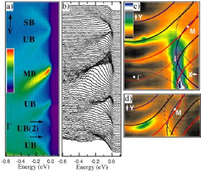
Figure 10: (a) Intensity $I({\bf k},\omega)$ and (b) EDCs along $\Gamma$Y measured on an optimally doped sample (T_c=90K) at T=40K with 33 eV photons polarized along $\Gamma$X. (c) Integrated intensity (-100 to +100 meV) covering the X and Y quadrants of the Brillouin zone. Data were collected on a regular lattice of ${\bf k}$ points (spacing $1^{\circ}$ along $\Gamma$X and $0.26^{\circ}$ along $\Gamma$Y). (d) Integrated intensity ($\pm$ 40 meV) as in (c), but in the normal state (T = 150K). Overlaid on (c) is the main band (black), $\pm$ umklapps (blue/red), and $\pm$ 2nd order umklapps (dashed blue/red lines) Fermi surfaces from a tight binding fit NORMAN_95a .

We now turn to panels (c,d) of Fig. 10 where we plot the integrated intensity within a $\pm$100 meV window about the chemical potential. We note the very rapid suppression of intensity beyond $\sim 0.8\Gamma$M saini97 , which does not occur in data taken with 22eV incident photons. This has led some authors chuang99 ; feng99 to suggest the existence of an electron-like Fermi surface with a crossing at this point. However, Fretwell et al.fretwell00 and independently Borisenko et al.borisenko00 have argued that this Fermi crossing along $(0,0)$ to $(\pi,0)$ is actually due to one of the umklapp bands, and the near optimally doped Fermi surface is indeed hole like as earlier shown by Ding et al.DING_96 .

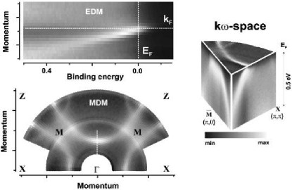
Figure 11: Upper panel: Energy distribution map from the $\Gamma-(\pi,\pi)$ direction in the Brillouin zone of Pb-doped BSCCO recorded at room temperature. Lower panel: momentum distribution map of Pb-doped BSCCO, recorded at room temperature (raw data). White horizontal dashed line represents a ${\bf k}_{F}$-EDC, vertical ones correspond to an $\it{E}_{F}$-MDC. In both cases the gray scale represents the photoemission intensity as indicated. The inset shows the three dimensional $(\it{k}_{x},\it{k}_{y},\omega)$ space, which is probed in ARPES of quasi-2D systems (from Ref.borisenko00 ).

This can be seen most clearly in Pb-doped samples, where the umklapp bands are not visible. In Fig. 11, we show the Fermi energy intensity map of Borisenko et al. borisenko00 , where the hole surface centered around $(\pi,\pi)$ and its shadow band partner are quite apparent.

One of the main reasons for the controversy surrounding the topology of the optimal doped Fermi surface is the fact that data taken at different incident photon energies $h\nu$ lead to different intensity patterns. Our assertion, based on Refs. fretwell00 ; mesot01 , is that the superlattice umklapp band is more noticeable at $h\nu=33$eV compared with 22 eV since matrix element effects suppress the main band intensity at 33 eV. For a detailed discussion about how to discriminate between a main band and superlattice Fermi crossing, we refer the reader to the cited papers, and also to Refs. DING_96 ; mesot01 for the use of polarization selection rules for this purpose.

Matrix Element Effects: There is an important general lesson to be learned from the above discussion which is equally relevant for the $n({\bf k})$ methods to be discussed below. Changes in the ARPES intensities (either integrated over a small energy window or over a large energy range) as a function of ${\bf k}$ can be strongly affected by matrix element effects. This is, of course, obvious from the expression for the the ARPES intensity: $I(\textbf{k},\omega)=I_{0}({\bf k};\nu;\hat{\bf A})f(\omega)A({\bf k},\omega)$. The key question is: after integration over the appropriate range in $\omega$, how do we differentiate between the ${\bf k}$ dependence coming from the matrix elements $I_{0}$ (which we are not interested in per-se) from the ${\bf k}$ dependence coming from the spectral function?

One possibility is to have a priori information about the matrix elements from electronic structure calculations BANSIL . But as we now show, even in the absence of such information, one can experimentally separate the effects of a strong ${\bf k}$-variation of the matrix element from a true Fermi surface crossing. The basic idea is to exploit the fact that changing the incident photon energy one only changes the ARPES matrix elements and not the spectral function (or the resulting momentum distribution) of the initial states.

We will use Bi2201 to illustrate our point since it has all the complications (points (1),(2) and (4)) listed above without the superlattice (point (3)). Fig. 12 (a), from Ref. mesot01 , shows the intensity (integrated over a large energy range) as a function of ${\bf k}$ for OD 23K Bi2201, and highlights the differences between data obtained at 22 eV and 34 eV incident photon energies. At 22 eV the maximum intensity occurs close to $(\pi,0)$ and decreases both toward $(0,0)$ and $(\pi,\pi)$, while at 34 eV there is a strong depression of intensity on approaching $(\pi,0)$, resulting in a shift of the intensity maximum away from $(\pi,0)$.

From the discussion of Section 2.4, we can write the integrated intensity as: $I(\textbf{k})=\int_{-\infty}^{+\infty}d\omega I(\textbf{k},\omega)=I_{0}({\bf k};\nu;{\bf A})n({\bf k})$. We attribute this loss in intensity around $(\pi,0)$ at 34 eV seen in Fig. 12(a) to strong ${\bf k}$-dependence of $I_{0}$ rather than $n({\bf k})$. Experimentally we prove this by showing that the EDCs at the same point in the Brillouin zone obtained at the two different photon energies show exactly the same lineshape, i.e. one can be rescaled onto the other as shown in Fig. 12(b). As an independent check of this, we have also shown that the symmetrization analysis leads to the same conclusion that there is no Fermi crossing along $(0,0)\to(\pi,0)$; see Fig. 9 of Ref. mesot01 .

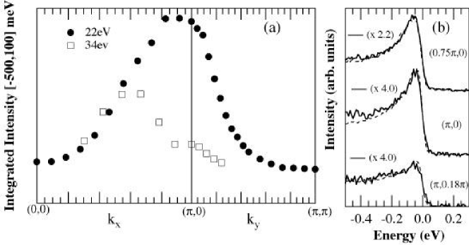
Figure 12: Bi2201-OD23K, (a) Integrated intensity (over the range is $-500$ to $100$ meV) along the $(0,0)\to(\pi,0)\to(\pi,\pi)$ directions for two incident photon energies $h\nu=$22 and 34 eV. (b) Comparison of the ARPES lineshape measured at 22 (dashed lines) and 34 eV (solid lines) at three different ${\bf k}$ points. One curve has been scaled by the multiplicative constant indicated to make it lie on top of the other.

For completeness, we note that another possible source of incident $h\nu$-dependence in ARPES is $k_{z}$-dispersion. If there was c-axis dispersion, different photon energies would probe initial states with different $k_{z}$ values consistent with energy conservation. However the scaling shown in Fig. 12(b) proves that it is the same two-dimensional ($k_{z}$-independent) initial state which is being probed in the data shown here, and the $h\nu$-dependence arises entirely from the different final states that the matrix element couples to.

Methods based on the Momentum Distribution Finally we turn to the use of the momentum distribution sum rule NK (discussed in Section 2.4) in determining the Fermi surface. In principle, locating the rapid variation of $n({\bf k})$ offers a very direct probe of the Fermi surface which we emphasize is not restricted to Fermi liquids. (The $T=0$ momentum distribution for known non-Fermi liquid systems, such as Luttinger liquids in one dimension, do show a inflection point singularity at ${\bf k}_{F}$.) However in practice, one needs to be very careful about the ${\bf k}$-dependence of the matrix elements, as clearly recognized in the original proposal NK .

Here we discuss two approaches using the $n({\bf k})$ method to obtain information about the Fermi surface. The first method is to study the $\bf k$-space gradient of the logarithm of the integrated intensity. The second method is to study the temperature-dependence of the integrated intensity and use the approximate sum rule NK $\partial n({\bf k}_{F})/\partial T=0$ discussed in Section 2.4.

The gradient method was used in our early work DING_96 ; CAMPUZANO_96 where ${\bf k}_{F}$ was estimated from the location of $\max\left|{\nabla_{\bf k}n({\bf k})}\right|$. The same method has also been successfully used later by other authors HUEFNER2 ; SCHABEL . In the presence of strong matrix element effects, it is even more useful to plot the magnitude of the logarithmic gradient: $|\nabla_{\bf k}I({\bf k})|/I({\bf k})$ which emphasizes the rapid changes in the integrated intensity. The logarithmic gradient filters out the less abrupt changes in the matrix elements and helps to focus on the intrinsic variations in $n({\bf k})$.

As an example we show in Fig. 13 the results mesot01 of such an analysis for an OD 0K Bi2201 sample. In the top panels (a) and (c) we show the integrated intensity $I({\bf k})$ around the $(\pi,0)$ point obtained at two different photon energies: 22 eV and 28 eV respectively. In the lower panels 11(b) and (d), we plot $|\nabla_{\bf k}I({\bf k})|/I({\bf k})$. Note that there are large differences between the two top panels, due to different matrix elements at 22 eV and 28 eV. However, as explained above, the logarithmic gradients in the bottom panels, which are more influenced by the intrinsic $n({\bf k})$, are much more similar. The Fermi surface can be clearly seen as two high intensity arcs curving away from the $(\pi,0)$ point. Once matrix element effects are taken care of, the Fermi surface results obtained at the two different photon energies are quite similar, and in good agreement with the results obtained from independent methods like symmetrization on the same data set mesot01 .

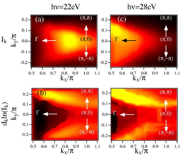
Figure 13: Bi2201-OD0K: (a and c) Integrated intensity (over -350 to +50 meV) $I({\bf k})$ measured at $\hbar\nu=$22 and 28 eV around the $(\pi,0)$ point. Notice that the intensity maximum depends strongly upon the photon energy $\hbar\nu$.(b and d) Corresponding gradient of the logarithm, $|\nabla_{\bf k}I({\bf k})|/I({\bf k})$, the maxima which correspond to Fermi crossings and clearly show that, independent of the photon energy, the Fermi surface consists of a hole barrel centered around $(\pi,\pi)$.

Our final method for the determination of a Fermi crossing goes back to the sum rule NK that we had introduced earlier, $\partial n({\bf k}_{F})/\partial T=0$. Assuming that the matrix elements are $T$-independent on the temperature scales of interest, this immediately implies the integrated intensity at (and only at) ${\bf k}_{F}$ is $T$-independent. In Section 2.4, we had used this sum rule to get confidence in the validity of the single-particle spectral function interpretation of ARPES by verifying at ${\bf k}_{F}$ assuming that ${\bf k}_{F}$ was known (by some other means). Now we can invert the logic: we can look at the $T$ dependence of the integrated intensity, and identify ${\bf k}_{F}$ as that point in ${\bf k}$-space where the integrated intensity is $T$-independent. This is illustrated in Fig. 14 from the work of Sato et al. sato01 , who determine ${\bf k}_{F}$ along the $(\pi,0)-(\pi,\pi)$ cut for a highly OD Bi2201 sample. The result is completely consistent with that obtained by other methods, such as “division by the Fermi function” on the same sample (see Fig. 4.2).

[width=.5]ns7.epsf

Figure 14: Temperature dependence of the integrated ARPES intensity $I({\bf k})$ along the $(\pi,0)-(\pi,\pi)$ cut, obtained by integrating the ARPES intensity from $-100$ to $100$ meV. (An angle-integrated temperature-independent background is subtracted before integration).

EDCs vs MDCs: To conclude this discussion, let us note a very recent development for determining $k_{F}$ and the near-$E_{f}$ dispersion based on the MDCs, which are plots of the ARPES intensity as a function of $k$ (in this case normal to the expected Fermi surface), at various fixed values of $\omega$. As shown in Section 2.5, the MDC peak position in the vicinity of the Fermi surface, i.e, near $({\bf k}={\bf k}_{F},\omega=0)$ is given by: $k=k_{F}+[\omega-\Sigma^{\prime}(\omega)]/v_{F}^{0}$.

Thus $k_{F}$ is determined by the peak location of the MDC at $\omega=0$. The fully renormalized Fermi velocity $v_{F}=v_{F}^{0}/[1-\partial\Sigma^{\prime}/\partial\omega]$ is given by the slope of the MDC peak dispersion. We note that the factor arising from the $k$-dependence of the self-energy is already included in $v_{f}^{0}$, so that $v_{f}^{0}=v_{f}^{\rm bare}[1+\partial\Sigma^{\prime}/\partial\varepsilon_{\bf k}]$. (To see this, note that the analysis of Section 2.5 can be easily generalized to retain the first order term $\partial\Sigma^{\prime}/\partial\varepsilon_{\bf k}$ without spoiling the Lorentzian lineshape of the MDC provided this $k$-dependence does not enter $\Sigma^{\prime\prime}$).

As discussed earlier, the above results derive from the Lorentzian lineshape of the MDC which arises when three conditions are satisfied: the matrix elements do not depend on $k$, the self energy does not depend on $k$ (except for the $(k-k_{F})$ variation of $\Sigma^{\prime}$ noted above) and dispersion can be linearized near the Fermi surface. The validity of these assumptions can be checked self-consistently by the Lorentzian MDC lineshape and the dispersion deduced from the data.

The significance of this approach is that, as emphasized by Kaminski et al.Adam01 , the dispersions of the EDC and MDC peak positions are actually different in the cuprates; see Fig. 53(a) in Section 7.7. This difference arises due to the non-Fermi liquid nature of the normal state, so that the EDC peak dispersion is not given by the condition $\omega-v_{F}^{0}(k-k_{F})-\Sigma^{\prime}=0$ but also involves in general $\Sigma^{\prime\prime}$. In contrast the MDC peak dispersion is rigorously described by the expression described above, and is much simpler to interpret.

We expect that the MDC method for determining the dispersion and $k_{F}$ which has thus far been used mainly along the zone diagonal, will eventually be the method of choice, except when one is very close to the bottom of the band where linearization fails.

4.3 Summary of Results on the Optimally Doped Fermi Surface:

We have discussed a large number of methods for determination of the Fermi surface in Bi2201 and Bi2212 in the previous subsection. These include: (a) dispersion of EDC peaks through $E_{f}$, (b) dispersion of peaks after division by the Fermi function, (c) symmetrization, (d) maps of intensities at $E_{f}$, (e) gradient of $n({\bf k})$, (f) $T$-dependence of $n({\bf k})$, and (g) MDC dispersion. In addition we also discussed using the $h\nu$-dependence of the data and polarization selection rules to eliminate matrix element effects and to identify superlattice Fermi crossings.

The reader might well ask: why so many different methods? The reason is that the development of all of these methods has taken place to deal with the complications of accurately identifying the Fermi surface in the presence of the four problems listed at the beginning of the preceding subsection. Each method has its pros and cons, so that some, like (b) and (c) require very accurate $E_{f}$ determination, which is not the case in (e) and (f) which use energy-integrated intensities. Most methods require dense sampling in $\bf k$ space, while method (f) requires in addition data at several temperatures.

Given the complications of the problem at hand it is important to look for crosschecks and consistency between various ways of determining the Fermi surface. We believe that for optimally doped Bi2201 and 2212 there is unambiguous evidence for a single hole barrel centered about the $(\pi,\pi)$ point enclosing a Luttinger volume of $(1+x)$ holes where $x$ is the hole doping. We discuss further below the issues of the doping-dependence of the Fermi surface and of bilayer splitting in Bi2212.

4.4 Extended Saddle Point Singularity

The very flat dispersion near the $(\pi,0)$ point observed in all of the data is striking. Specifically, along $(0,0)$ to $(\pi,0)$ there is an intense spectral peak corresponding to the main band, which disperses toward $E_{F}$ but stays just below it. This is often called the “flat band” or “extended saddle point”, and appears to exist in all cuprates, though at different binding energies in different materials GOFRON ; DESSAU_93 ; SHEN_REVIEW .

In our opinion this flat band is not a consequence of the bare electronic structure, but rather a many-body effect, because a tight-binding description of such a dispersion requires fine-tuning (of the ratio of the next-near neighbour hopping to the near-neighbour hopping) which would be unnatural even in one material, let alone many.

An important related issue is whether this flat band leads to a singular density of states. It is very important to recognize that, while Fig. 8(b) looks like a conventional band structure, the dispersing states whose “peak positions” are plotted are extremely broad, with a width comparable to binding energy, and these simply cannot be thought of as quasiparticles. This general point is true at all ${\bf k}$’s, but specifically for the flat band region it has the effect of spreading out the spectral weight over such a broad energy range that any singularity in the DOS would be washed out. This is entirely consistent with the fact that other probes (tunneling, optics, etc.) do not find any evidence for a singular density of states either.

4.5 Bilayer Splitting?

On very general grounds, one expects that the two CuO₂ layers in a unit cell of Bi2212 should hybridize to produce two electronic states which are even and odd under reflection in a mirror plane mid-way between the layers. Where are these two states? Why then did we find only one main “band” and only one Fermi surface in Bi2212?

Let us first recall the predictions of electronic structure calculations BAND_THEORY . In systems like Bi2212, the intra-bilayer hopping as a function of the in-plane momentum ${\bf k}$ is of the form OKA ; ILT $t_{\perp}({\bf k})=-t_{z}(\cos k_{x}-\cos k_{y})^{2}$. Thus the two bilayer states are necessarily degenerate along the zone diagonal. However they should have a maximum splitting at $\bar{M}=(\pi,0)$ of order 0.25 eV, which may be somewhat reduced by many-body interactions.

Depending on the exact doping levels and on the presence of Bi-O Fermi surface pockets, which are neither treated accurately in the theory nor observed in the ARPES data, we must obtain one of the two following situations: (1) the bilayer antibonding (A) state is unoccupied while the bonding (B) state is occupied at $(\pi,0)$. This would lead to an A Fermi crossing along $(0,0)-(\pi,0)$ and a B Fermi crossing along $(\pi,0)-(\pi,\pi)$. As described at great length above we did not find evidence for a main band Fermi crossing along $(0,0)-(\pi,0)$ at least for the near optimal doped sample, therefore this possibility is ruled out.

(2) The second possibility is that both the A and B bilayer states are occupied at the $(\pi,0)$. In this case, there should be two (in principle, distinct) Fermi crossings along $(\pi,0)-(\pi,\pi)$, although they might be difficult to resolve in practice. Nevertheless, one would definitely expect to see two distinct occupied states at the $(\pi,0)$ point. Unfortunately, the normal state spectrum at $(\pi,0)$ is so broad in the optimally doped and underdoped materials that it is hard to make a clear case for bilayer splitting. Thus an effort was made to search for this effect in the superconducting state at $T\ll T_{c}$, when a sharp feature (quasiparticle peak) is seen (see Fig. 15) and one might hope that the bilayer splitting should be readily observable.

[width=.5]ns8.epsf

Figure 15: Low temperature (T=13K) EDC’s of near optimal $T_{c}=87$K Bi2212 at $(\pi,0)$ for various incident photon angles. The solid (dashed) line is $18^{\circ}$ ($85^{\circ}$) from the normal. The inset shows the height of the sharp peak for data normalized to the broad bump, at different incident angles.

The issue then is how to interpret the peak-dip-hump structure seen in the ARPES lineshape at $(\pi,0)$ in Fig. 15. The peak-dip-hump structure will be discussed at length in Section 7 below. Nevertheless, here we will briefly address the question of whether: (I) the peak and the hump are the two bilayer split states, which are resolved below $T_{c}$ once the peak becomes sharp? Or (II) is the non-trivial line shape due to many-body effects in a single spectral function $A({\bf k},\omega)$?

Three pieces of evidence will be offered in favor of hypothesis (II) as opposed to (I), so that no bilayer spliting is observable even in the superconducting state of near optimal doped Bi2212. The first evidence comes from studying the polarization dependence of the ARPES matrix elements. For case (I) there are two independent matrix elements which, in general, should vary differently with photon polarization ${\bf A}$, and thus the intensities of the two features should vary independently as ${\bf A}$ is varied. On the other hand, for case (II), the intensities of the two features are governed by a single matrix element. As shown in Fig. 15 it was found in Ref. DING_96 that by varying the z-component of ${\bf A}$, the peak and hump intensities scale together, and thus the peak-dip-hump are all part of a single spectral function for Bi2212.

A second piece of evidence comes from a comparison Mike97 of the normal and superconducting state dispersions near the $(\pi,0)$ point, which will be discussed in detail in connection with Figs. 42 and 43 of Section 7.4. From these data, we argue that there is no evidence for a feature above $T_{c}$, which would correspond to the dispersionless quasiparticle peak below $T_{c}$. Thus the dispersionless peak must be of many-body origin.

The third and final piece of evidence comes from both ARPES and SIS tunneling. In the ARPES data JC99 shown in Fig. 49 of Section 7.6 one sees the striking fact that while the energy scales of both the quasiparticle peak and the $(\pi,0)$ hump increase with underdoping, their ratio is essentialy doping independent. Since the location of the peak is the (maximum) superconducting gap – as discussed in detail in Section 5 – the $(\pi,0)$ hump energy scales with the gap. SIS tunneling data also finds the same correlation on a very wide range of materials (including some which have a single CuO plane) whose gap energies vary by a factor of 30 JohnZ96 . This provides very strong evidence that both the peak and hump are related to many-body effects and not manifestations of bilayer spliting.

We note that Anderson ANDERSON had predicted that many-body effects within a single layer could destroy both the quasiparticles and the coherent bilayer splitting in the normal state. But why the splitting should not be visible in the superconducting state, where sharp quasiparticles do exist, is not clear from a theoretical point of view.

Recently, the above picture has been challenged by a number of authors BILAY1 ; BILAY2 ; BILAY3 . What has become clear is that bilayer splitting is indeed present for heavily overdoped Bi2212 samples, and has been seen now by several groups, including our own. In Fig. 16, we show (a) the bilayer split Fermi surfaces and (b) the bilayer split EDCs observed by the Stanford group for a heavily overdoped ($T_{c}$=65K) Bi2212 sample. Note that the bilayer splitting can even be seen in the umklapp bands. The resulting dispersion is reproduced in Fig. 17, where one sees that the momentum dependence of the splitting follows that expected from electronic structure considerations OKA ; ILT .

[width=.5]feng1.epsf

Figure 16: (a) Bilayer-split Fermi surfaces of heavily overdoped OD65; the two weaker features are their superstructure counter parts. Solid and dashed lines represent the bonding and antibonding Fermi surfaces, respectively. (b) Normal state photoemission spectra of Bi2212 taken at $(\pi,0)$ for three different doping levels. Data were taken with $h\nu$ = 22.7 eV photon. Bars indicate identified feature positions, and triangles indicate possible feature positions. (from Ref. BILAY1 ).

[width=.5]feng2.epsf

Figure 17: (a) Dispersion extracted from heavily overdoped OD65. (b) Energy splitting along the antibonding Fermi surface, which is obtained from data shown in Fig.16. It is simply the binding energy of the bonding band, since the binding energy of the antibonding band is zero at its Fermi surface. The curve is $\frac{1}{2}t_{\bot,\exp}[\cos(k_{x}a)-\cos(k_{y}a)]^{2}$, where $t_{\bot,\exp}$ = 44 $\pm$5 meV. Error bars are due to the uncertainties in determining the energy position (from Ref.BILAY1 ).

How this effect evolves as a function of doping, though, is still controversial. In particular, if it is present for optimal doping, it is difficult to resolve. Moreover, some authors who advocate bilayer splitting still argue that the peak/dip/hump structure in the superconducting state is largely a many-body effect BILAY1 as we adovcate here. This is supported by the fact that the same lineshape is seen in trilayer Bi2223 TRILAYER , where one would expect three features if layer splitting were causing these effects. And similar lineshapes have been seen by tunneling in single layer systems, in support of a many-body interpretation. The reader is refered to Ref. RMP , where the issue of bilayer splitting is discussed in greater detail than here.

5 Superconducting Energy Gap

In this Section, we will first establish how the superconducting (SC) gap manifests itself in ARPES spectra, and then directly map out its variation with ${\bf k}$ along the Fermi surface. This is the only available technique for measuring the momentum dependence of the energy gap, and complements phase-sensitive tests of the order parameter symmetry OP_SYMMETRY . Thus ARPES has played an important role SHEN_93 , DING_GAP in establishing the $d$-wave order parameter in the high $T_{c}$ superconductors OP_SYMMETRY . At the end of the Section, we will discuss the doping dependence of the SC gap and its anisotropy, and the implications of this study for various low temperature experiments like thermal conductivity and penetration depth.

5.1 Particle-Hole Mixing

To set the stage for the experimental results it may be useful to recall particle-hole (p-h) mixing in the BCS framework (even though, as we shall see in Section 7, there are aspects of the data which are dominated by many body effects beyond weak coupling BCS theory). The $BCS$ spectral function is given by

$$A({\bf k},{\omega})=u_{\bf k}^{2}{\Gamma}/{\pi}(({\omega}-E_{\bf k})^{2}+{\Gamma}^{2})+v^{2}_{\bf k}{\Gamma}/{\pi}(({\omega}+E_{\bf k})^{2}+{\Gamma}^{2})$$ (15)

where the coherence factors are $v^{2}_{\bf k}=1-u_{\bf k}^{2}={1\over 2}(1-{\epsilon}_{\bf k}/E_{\bf k})$ and $\Gamma$ is a phenomenological linewidth. The normal state energy ${\epsilon}_{\bf k}$ is measured from $E_{f}$ and the Bogoliubov quasiparticle energy is $E_{\bf k}=\sqrt{\epsilon_{\bf k}^{2}+|\Delta({\bf k})|^{2}}$, where $\Delta({\bf k})$ is the gap function. Note that only the second term in Eq. 15, with the $v_{\bf k}$-coefficient, would be expected to make a significant contribution to the EDCs at low temperatures.

[width=.3]bcsmodel.epsf

Figure 18: Schematic dispersion in the normal (thin line) and superconducting (thick lines) states following BCS theory. The thickness of the superconducting state lines indicate the spectral weight given by the BCS coherence factors $u$ and $v$.

In the normal state above $T_{c}$, the peak of $A({\bf k},{\omega})$ is at $\omega=\epsilon_{\bf k}$ as can be seen by setting $\Delta=0$ in Eq. 15. We would thus expect to see in ARPES a spectral peak which disperses through zero binding energy as ${\bf k}$ goes through ${\bf k}_{F}$ (the Fermi surface). In the superconducting state, the spectrum changes from $\epsilon_{\bf k}$ to $E_{\bf k}$; see Fig. 18. As ${\bf k}$ approaches the Fermi surface the spectral peak shifts towards lower binding energy, but no longer crosses $E_{f}$. Precisely at ${\bf k}_{F}$ the peak is at $\omega=|\Delta({\bf k}_{F})|$, which is the closest it gets to $E_{f}$. This is the manifestation of the gap in ARPES. Further, as ${\bf k}$ goes beyond ${\bf k}_{F}$, in the region of states which were unoccupied above $T_{c}$, the spectral peak disperses back, receding away from $E_{f}$, although with a decreasing intensity (see Eq. 15). This is the signature of p-h mixing.

[width=.5]particlehole.epsf

Figure 19: (a) Superconducting state and (b) normal state EDC’s for a near optimal $T_{c}=87$K Bi2212 sample for a set of ${\bf k}$ values (in units of $1/a$) shown in the Brillouin zone at the top. Note the different binding energy scales in panels (a) and (b).

Experimental evidence for particle-hole mixing in the SC state was first given in Ref. CAMPUZANO_96 . In Fig. 19 we show normal and SC state spectra for Bi2212 for ${\bf k}$’s along the cut shown in the inset. In the normal state data in panel (b) we see the electronic state dispersing through $E_{f}$: the ${\bf k}$’s go from occupied (top of panel) to unoccupied states (bottom of panel). The normal state dispersion is plotted as black dots in Fig. 20 (b). The ${\bf k}_{F}$ obtained from this dispersion is in agreement with that estimated from the $|\nabla_{{\bf k}}n({\bf k})|$ analysis of the normal state data shown in Fig. 20 (a).

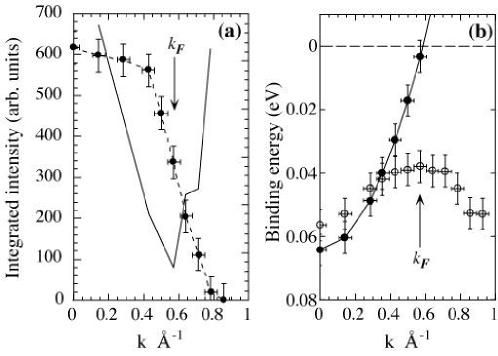
Figure 20: (a) Integrated intensity versus ${{\bf k}}$ from the normal state data of Fig. 19 (b) shown by black dots gives information about the momentum distribution $n({\bf k})$. The derivative of the integrated intensity is shown by the black curve (arbitrary scale). The Fermi surface crossing ${\bf k}={\bf k}_{F}$ is identified by the minimum in the derivative. (b) Normal state dispersion (closed circles) and SC state dispersion (open circles) obtained from EDC’s of Fig. 19. Note the back-bending of the SC state dispersion for ${\bf k}$ beyond ${\bf k}_{F}$ which is a clear indication of particle-hole mixing. The SC state EDC peak position at ${\bf k}_{F}$ is an estimate of the SC gap at that point on the Fermi surface.

We see from Fig. 19 (a) that the SC state spectral peaks do not disperse through the chemical potential, rather they first approach $\omega=0$ and then recede away from it. The difference between the normal and SC state dispersions is clearly shown in Fig. 20 (b).

There are three important conclusions to be drawn from Fig. 20 (b). First, the bending back of the SC state spectrum for ${\bf k}$ beyond ${\bf k}_{F}$ is direct evidence for p-h mixing in the SC state. Second, the energy of closest approach to $\omega=0$ is related to the SC gap that has opened up at the FS, and a quantitative estimate of this gap will be described below. Third, the location of closest approach to $\omega=0$ (“minimum gap”) coincides, within experimental uncertainties, with the ${\bf k}_{F}$ obtained from analysis of normal state data.

In fact by taking cuts in ${\bf k}$-space which which are perpendicular to the normal state Fermi surface one can map out the “minimum gap locus” in the SC state, or for that matter in any gapped state (e.g., the pseudogap regime to be discussed in the following Section). We emphasize that particle-hole mixing leads to the appearance of the “minimum gap locus” and this locus in the gapped state gives information about the underlying Fermi surface. (By this we mean the Fermi surface on which the SC state gap appears below $T_{c}$). In fact, the observation of p-h mixing in the ARPES spectra is a clear way of asserting that the gap seen by ARPES is due to superconductivity rather than of some other origin, e.g., charge- or spin-density wave formation.

5.2 Quantitative Gap Estimates

The first photoemission measurements of the SC gap in the cuprates was by Imer et al.IMER89 using angle-integrated photoemission, and by Olson and coworkers olson2 using angle-resolved photoemission. The first identification of a large gap anisotropy consistent with d-wave pairing was made by Shen and coworkers SHEN_93 . Ding et al.DING95 ; DING_GAP subsequently made quantitative fits to the SC state spectral function to study the gap anisotropy in detail.

We now discuss the quantitative extraction of the gap at low temperatures ($T\ll T_{c}$) following Ding et al.DING_GAP . In Fig. 22, we show the $T=13$K EDCs for an 87K $T_{c}$ sample for various points on the main band FS in the $Y$-quadrant. Each spectrum shown corresponds to the minimum observable gap along a set of ${\bf k}$ points normal to the FS, obtained from a dense sampling of ${\bf k}$-space DENSE . We used 22 eV photons in a $\Gamma Y\perp$ polarization, with a 17 meV (FWHM) energy resolution, and a ${\bf k}$-window of radius 0.045$\pi/a^{*}$.

[width=.5]gaparoundfs.epsf

Figure 21: Bi2212 spectra (solid lines) for an 87K $T_{c}$ sample at 13K and Pt spectra (dashed lines) versus binding energy (meV) along the Fermi surface in the $Y$ quadrant. The photon polarization and BZ locations of the data points are shown in inset to Fig. 22

The simplest gap estimate is obtained from the mid-point shift of the leading edge of Bi2212 relative to a good metal (here Pt) in electrical contact with the sample. This has no obvious quantitative validity, since the Bi2212 EDC is a spectral function while the polycrystalline Pt spectrum (dashed curve in Fig. 21) is a weighted density of states whose leading edge is an energy-resolution limited Fermi function. We see that the shifts (open circles in Fig. 22) indicate a highly anisotropic gap which vanishes in the nodal directions, confirming earlier results by Shen et al. SHEN_93 . These results are qualitatively similar to one obtained from the fits described below.

Next we turn to modeling DING95 ; DING_GAP the SC state data in terms of spectral functions. It is important to ask how can we model the non-trivial line shape (with the dip-hump structure at high $\omega$) in the absence of a detailed theory, and, second, how do we deal with the extrinsic background? We argue as follows: in the large gap region near $(\pi,0)$, we see a linewidth collapse for frequencies smaller than $\sim 3\Delta$ upon cooling well below $T_{c}$. Thus for estimating the SC gap at the low temperature, it is sufficient to look at small frequencies, and to focus on the coherent piece of the spectral function with a resolution-limited leading edge. (Note this argument fails at higher temperatures, e.g., just below $T_{c}$). This coherent piece is modeled by the BCS spectral function, Eq. 15.

The effects of experimental resolution are taken into account via

$${\tilde{I}}({\bf k},\omega)=I_{0}\int_{\delta{\bf k}}d{\bf k}^{\prime}\int_{-\infty}^{+\infty}d\omega^{\prime}R(\omega-\omega^{\prime})f(\omega^{\prime})A({\bf k}^{\prime},\omega^{\prime})$$ (16)

where $R(\omega)$, the energy resolution, is a normalized Gaussian and $\delta{\bf k}$ is the ${\bf k}$-window of the analyzer. In so far as the fitting procedure is concerned, all of the incoherent part of the spectral function is lumped together with the experimental background into one function which is added to the ${\tilde{I}}$ above. Since the gap is determined by fitting the resolution-limited leading edge of the EDC, its value is insensitive to this drastic simplification. To check this, we have made an independent set of fits to the small gap data where we do not use any background fitting function, and only try to match the leading edges, not the full spectrum. The two gap estimates are consistent within a meV. Once the insensitivity of the gap to the assumed background is established, there are only two free parameters in the fit at each ${\bf k}$: the overall intensity $I_{0}$ and the gap $|\Delta|$; the dispersion ${\epsilon}_{\bf k}$ is known from the normal state study, the small linewidth $\Gamma$ is dominated by the resolution.

The other important question is the justification for using a coherent spectral function to model the rather broad EDC along and near the zone diagonal. As far as the early data being discussed here is concerned, such a description is self-consistent DING95 ; DING_GAP , though perhaps not unique, with the entire width of the EDC accounted for by the large dispersion (of about 60 meV within our ${\bf k}$-window) along the zone diagonal. More recent data taken along $(0,0)$ to $(\pi,\pi)$ with a momentum resolution of $\delta{\bf k}\simeq 0.01\pi/a^{*}$ fully justifies this assumption by resolving coherent nodal quasiparticles in the SC state; see Section 7.7.

[width=.5]dwavegap.epsf

Figure 22: $Y$ quadrant gap in meV versus angle on the Fermi surface (filled circles) from fits to the data of Fig. 21. Open symbols show leading edge shift with respect to Pt reference. The solid curve is a d-wave fit to the filled symbols.

The gaps extracted from fits to the spectra of Fig. 21 are shown as filled symbols in Fig. 22. For a detailed discussion of the the error bars (both on the the gap value and on the Fermi surface angle), and also of sample-to-sample variations in the gap estimates, we refer the reader to Ref. DING_GAP . The angular variation of the gap obtained from the fits is in excellent agreement with $|\cos(k_{x})-\cos(k_{y})|$ form. The ARPES experiment cannot of course measure the phase of the order parameter, but this result is in strong support of $d_{x^{2}-y^{2}}$ pairing OP_SYMMETRY . Such an order parameter arises naturally in theories with strong correlations and/or antiferromagnetic spin fluctuations DWAVE . Moreover, the functional form of the anisotropy we find is consistent with electrons in the Cooper pair residing on neighboring Cu sites. That is, ARPES gives information on the spatial range of the pair interaction which is difficult to obtain from other techniques.

Finally we comment on the temperature dependence of the gap. Unfortunately with increasing temperature the linewidth grows and a simple BCS-type modeling (valid for $T\ll T_{c}$) of just the coherent part of the spectral function is not possible. While $T$-dependence of the leading edge can certainly be used as a rough guide, this estimate is affected by both the gap and the linewidth (the diagonal self-energy). We will discuss methods for modeling the SC state data in Section 7.

For completeness, we add a remark clarifying the earlier observation of two nodes in the $X$-quadrant DING95 , and the related non-zero gap along $\Gamma X$ in the $\Gamma X||$ geometry DING95 ; KELLY . It was realized soon afterwards that these observations were related to gaps on the superlattice bands NORMAN_95b , and not on the main band. To prove this experimentally, the $X$-quadrant gap has been studied in the $\Gamma X\perp$ geometry DING_GAP and found to be consistent with $Y$-quadrant $d_{x^{2}-y^{2}}$ result described above.

5.3 Doping Dependence of the SC Gap

There are two important issues to be addressed about the doping dependence: How does the maximum gap change with doping? and how does the gap anisotropy evolve with doping?

ARPES results on underdoped samples show that the maximum gap increases HARRIS_96 ; SNS97 with decreasing hole concentration. For a recent compilation of gap versus doping results JC99 in Bi2212, see Fig. 49 of Section 7.6. Identical results have also been obtained by tunneling spectroscopy STM_GAP . This was at first quite unexpected since $T_{c}$ decreases as one underdopes from optimality. The fact that $2\Delta/k_{B}T_{c}$ is not constant with doping and can become an order of magnitude larger than its BCS weak-coupling value is very clear evidence that the SC phase transition on the underdoping side is qualitatively different from the BCS transition, a point that we will return to in the next Section on pseudogaps.

We next turn to the question of the SC gap anisotropy as a function of doping. In this case it is the behavior of the gap in the vicinity of the node which is the most important since all low temperature $T\ll T_{c}$ thermodynamic and transport properties are controlled by thermal excitation of quasiparticles in the vicinity of the nodes (where the SC gap vanishes on the Fermi surface). These low energy excitations have a Dirac-like spectrum $E({\bf k})=\sqrt{v_{F}^{2}k_{\perp}^{2}+v_{2}^{2}k_{\parallel}^{2}}$ where $k_{\perp}$ ($k_{\parallel}$) are the components of the ${\bf k}$ perpendicular (tangential) to the Fermi surface, and measured from the nodal point. Here $v_{F}$ is the nodal Fermi velocity controlling the dispersion perpendicular to the Fermi surface, while $v_{2}=\partial\Delta_{\bf k}/\partial k_{\parallel}$ is the the gap slope at the nodal point.

The density of states for low energy excitations is then given by $N(\omega)=2\omega/(\pi v_{F}v_{2})$ for $\omega\ll\Delta$ (in units where $\hbar=1$). This leads to characteristic temperature dependences for various low temperature properties with coefficients essentially determined by $v_{F}$ and $v_{2}$. Specifically for $T\ll T_{c}$, the specific heat goes like $C(T)=c_{1}T/(v_{F}v_{2})$; the thermal conductivity goes like $\kappa(T)/T=c_{2}\left(v_{F}/v_{2}+v_{2}/v_{F}\right)$ and the superfluid density goes like $\rho_{s}(T)=\rho_{s}(0)-c_{3}(v_{F}/v_{2})T$. Here $c_{1}$ and $c_{2}$ are known constants while $c_{3}$ contains (apriori unknown) multiplicative Fermi liquid parameters MILLIS ; DURST .

Clearly ARPES has a unique ability to independently measure both $v_{F}$, using the dispersion of the nodal quasiparticle, and $v_{2}$, using the slope of the SC gap at the node. One can then make detailed comparison with various bulk measurements, and thereby test the validity of the description of the low temperature properties of the SC state in terms of weakly interacting quasiparticles MILLIS ; DURST ; CHIAO . This is particularly important given the lack of sharply defined quasiparticles in the normal state of the cuprates.

With these motivations in mind, a detailed measurement of the shape of the superconducting gap in Bi2212 as a function of doping was carried out by Mesot et al.MESOT . Although these measurements were carried out at a time when the energy and momentum resolutions were lower than those currently available, they still give useful information because the gap over the full range of angles over the irreducible zone was measured. Using the simple BCS spectral function fits (described above) and taking into account the measured dispersion and the known energy and momentum resolutions, Mesot et al.found the results shown in Fig. 23. The simple d-wave gap $\Delta=\Delta_{0}\cos(2\phi)$ (Fig. 22) is modified by the addition of the first harmonic $\Delta_{\bf k}=\Delta_{\rm max}[B\cos(2\phi)+(1-B)\cos(6\phi)]$, with $0\leq B\leq 1$. Note that the $\cos(6\phi)$ term in the Fermi surface harmonics can be shown to be closely related to the tight binding function $\cos(2k_{x})-\cos(2k_{y})$, which represents next nearest neighbours interaction, just as $\cos(2\phi)$ is closely related to the near neighbor pairing function $\cos(k_{x})-\cos(k_{y})$. From Fig. 23 we find that while the overdoped data are consistent with $B\simeq 1$, the parameter $B$ decreases as a function of underdoping.

[width=.5]gapvsdoping.epsf

Figure 23: Values of the superconducting gap as a function of the Fermi surface angle $\phi$ obtained for a series of Bi2212 samples with varying doping. Note two different UD75K samples were measured, and the UD83K sample has a larger doping due to sample agingDING_97 . The solid lines represent the best fit using the gap function: $\Delta_{k}=\Delta_{\rm max}[B\cos(2\phi)+(1-B)\cos(6\phi)]$ as explained in the text. The dashed line in the panel of an UD75K sample represents the gap function with B=1.

Before discussing the doping dependence of the results in detail, let us first look at the comparisons between ARPES and other probes near optimality. Low temperature specific heat data on Bi2212 is not available, but the thermal conductivity has been measured by Taillefer and coworkers CHIAO on an optimal $T_{c}=89$K sample. Now one can use the $\kappa/T$ formula given above with the coefficient $c_{2}=k_{B}^{2}n/3\hbar d$, where $n/d$ is the stacking density of CuO₂ planes. It is important to note that $c_{2}$ is not renormalized by either vertex corrections or Fermi liquid parameters DURST . Thus one infers $v_{F}/v_{2}=19$ from the thermal transport data CHIAO , which is in remarkable agreement with the ARPES estimate MESOT of $v_{F}/v_{2}\simeq 20$ coming from the measured values of $v_{F}=2.5\times 10^{7}$ cm/s and $v_{2}=1.2\times 10^{6}$ cm/s for the near optimal $T_{c}=87$K sample of Fig. 23. (We note that in Ref. MESOT we used the notation $v_{\Delta}$ for one-half the gap slope at the node, which is related to $v_{2}$ defined above by $v_{2}=2v_{\Delta}/\hbar k_{F}$.)

The comparison of ARPES results with the slope of the superfluid density $\rho_{s}\sim 1/\lambda^{2}$ obtained from penetration depth measurements is more complicated, as discussed in more detail in Ref. MESOT , for two reasons. Experimentally, there seem to be discrepancies between the $d\lambda^{-2}/dT$ results of various groups, and theoretically the slope of $\rho_{s}$ is renormalized by doping-dependent Fermi liquid parameters MILLIS ; DURST which are not known apriori. These parameters characterize the residual interactions between the nodal quasiparticles in the superconducting state. Thus, e.g., even at optimality the slope $d\lambda^{-2}/dT$ obtained using the ARPES estimate of $v_{F}/v_{2}$ and ignoring Fermi liquid renormalization is almost three times as large as the experimentally measured value of $d\lambda^{-2}/dT$ in near optimal Bi2212 LAMBDA . This indicates the importance of Fermi liquid renormalizations in order to make a quantitative comparison. For more details on the doping dependence of these renormalizations, see Ref. MILLIS ; MESOT ; M2S .

Finally, let us return to the doping dependence of the results of Fig. 23. In contrast to the maximum gap (at the $(\pi,0)-(\pi,\pi)$ Fermi surface crossing) increasing as a function of underdoping, noted earlier, we see the gap slope at the node, which determines $v_{2}$, decreasing with underdoping. This is a result of the doping dependence of the $B$ parameter introduced above.

This surprising observation raises several questions. First, could the flattening at the node be, in fact, evidence for a “Fermi arc”, a line of gapless excitations, in the underdoped materials, especially since such arcs are seen above $T_{c}$ (See Sect. 6.3 for further discussion of Fermi arcs in underdoped materials). Given the error bars on gap estimates in Fig. 23, it is impossible to rule out arcs in all the samples. Nevertheless, it is clear that there are samples (especially OD87K, UD80K and UD75K) where there is clear evidence in favor of a point node rather than an arc at low temperatures. Furthermore, it is very important to note that a linear $T$ dependence of $\rho_{s}(T)$ at low temperature, for all doping levels, in clean samples gives independent evidence for point nodes, at least in YBCO HARDY .

Second, is the change in gap anisotropy intrinsic, or related to impurity scatteringHAAS ? We can eliminate the latter explanation on two grounds. The maximum gap increases as the doping is reduced, opposite to what would be expected from pair breaking due to impurities. Also, impurity scattering is expected to lead to a characteristic “tail” to the leading edge FN , for which there is no evidence in the observed spectra.

Thus the flattening near the nodes with underdoping does appear to be an intrinsic feature which may be related to the increased importance of longer range pairing interactions as one approaches the insulator. It would be of great interest to study the details of the doping dependence of the gap anisotropy with the new Scienta detectors which have greatly improved energy and momentum resolution.

6 Pseudogap

In this Section we describe one of the most fascinating developments in the study of high $T_{c}$ superconductors: the appearance of a pseudogap above $T_{c}$ which is seen most prominently on the underdoped side of the cuprate phase diagram. Briefly the “pseudogap” phenomenon is the loss of low energy spectral weight in a window of temperatures $T_{c}<T<T^{*}$; see Fig. 24. The pseudogap regime has been probed by many techniques like NMR, optics, transport, tunneling, $\mu$SR and specific heat; for reviews and references, see Refs. TIMUSK ; MR_VARENNA . ARPES, with its unique momentum-resolved capabilities, has played a central role in elucidating the pseudogap phenomenon MARSHALL ; LOESSER ; DING_NATURE ; DING_97 ; Nature98 .

We will discuss in this Section ARPES results on the anisotropy of the pseudogap, its $T$-dependence, its doping dependence, and its effect on the normal state Fermi surface. We emphasize that for the most part we will focus on the “low energy” or leading edge pseudogap, and only mention ARPES evidence for the “high energy pseudogap” toward the end. We will conclude the Section with a summary of the constraints put by the ARPES data on various theoretical descriptions of the pseudogap.

[width=.5]phase_diagram.epsf

Figure 24: $T^{*}$ (triangles for determined values and squares for lower bounds) and $T_{c}$ (dashed line) as a function of hole doping $x$. The $x$ values for a measured $T_{c}$ were obtained by using the empirical relation $T_{c}/T_{c}^{max}=1-82.6(x-0.16)^{2}$ PRES with $T_{c}^{max}=$95 K. Also shown is the low temperature (maximum) superconducting gap $\Delta(0)$ (circles). Note the similar doping trends of $\Delta(0)$ and $T^{*}$.

6.1 Pseudogap near $(\pi,0)$

In the underdoped materials, $T_{c}$ is suppressed by lowering the carrier (hole) concentration as shown in Fig. 24. In the samples used by our group DING_NATURE ; DING_97 ; Nature98 underdoping was achieved by adjusting the oxygen partial pressure during annealing the float-zone grown crystals. These crystals also have structural coherence lengths of at least 1,250$\AA$ as seen from x-ray diffraction, and optically flat surfaces upon cleaving, similar to the slightly overdoped $T_{c}$ samples discussed above. We denote the underdoped (UD) samples by their onset $T_{c}$: the 83K sample has a transition width of 2K and the highly underdoped 15K and 10K have transition widths $>5$K. Other groups have also studied samples where underdoping was achieved by cation substitution MARSHALL ; LOESSER .

We now contrast the remarkable properties of the underdoped samples with the near-optimal Bi2212 samples which we have been mainly focusing on thus far. We will first focus on the behavior near the $(\pi,0)$ point where the most dramatic effects occur, and come back to the very interesting ${\bf k}$-dependence later. In Fig. 25 SNS97 we show the $T$-evolution of the ARPES spectrum at the $(\pi,0)\to(\pi,\pi)$ Fermi crossing for an UD 83K sample. At sufficiently high temperature, the leading edge of the UD spectrum at ${\bf k}_{F}$ and the reference Pt spectrum coincide, but below a crossover temperature $T^{*}\simeq 180$K the leading edge midpoint of the spectrum shifts below the chemical potential. In Fig. 25 one can clearly see a loss of low energy spectral weight at 120K and 90K. It must be emphasized that this gap-like feature is seen in the normal (i.e., non-superconducting) state for $T_{c}=83K<T<T^{*}=180K$.

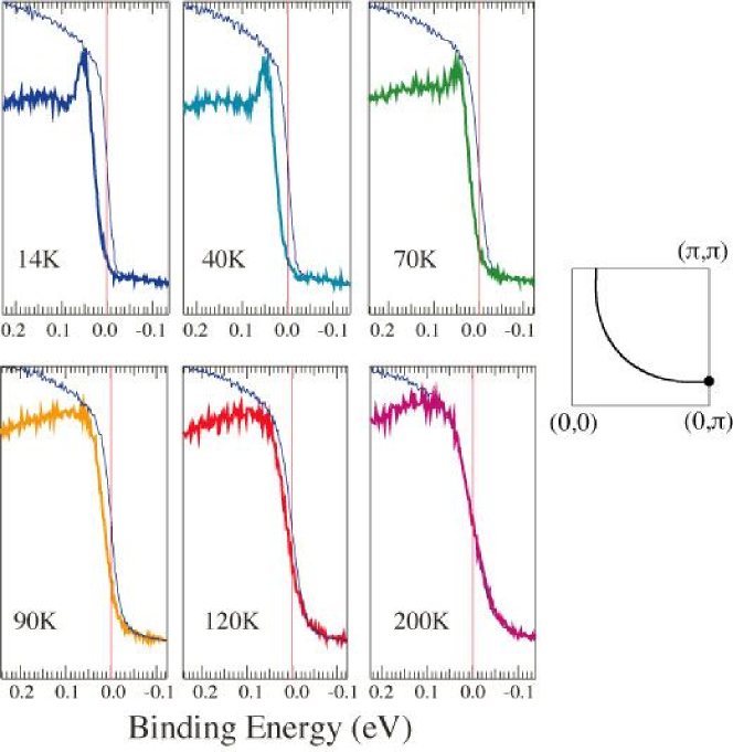
Figure 25: ARPES spectra along the $(\pi,0)\to(\pi,\pi)$ direction for an 83 K underdoped sample at various temperatures (solid curves). The thin curves in each panel are reference spectra from polycrystalline Pt used to accurately determine the zero of binding energy at each temperature.

The doping dependence of the temperature $T^{*}$, below which a leading-edge pseudogap appears near $(\pi,0)$, is shown in Fig. 24. Remarkably $T^{*}$ increases with underdoping, in sharp contrast with $T_{c}$, but very similar to the low temperature SC gap, a point we will return to at the end of the Section. The region of the phase diagram between $T_{c}$ and $T^{*}$ is called the pseudogap region.

It is important to emphasize that our understanding of the lightly UD samples (e.g., the UD 83K sample) is the best among the UD materials. In such samples all three regimes – the SC state below $T_{c}$, the pseudogap regime between $T_{c}$ and $T^{*}$ and the gapless “normal” regime above $T^{*}$ – can be studied in detail. In contrast, in the heavily UD samples (e.g. the UD 10K and UD 15K samples), not only is the SC transition broad, one also has such low $T_{c}$’s and such high $T^{*}$’s that only the pseudogap regime is experimentally accessible. Nevertheless, the results on the heavily underdoped samples appear to be a natural continuation of the weakly underdoped materials and the results (the trends of gap and $T^{*}$) on the low $T_{c}$ samples are in qualitative agreement with those obtained from other probes (see Ref. TIMUSK ; MR_VARENNA ).

The $T$-dependence of the leading-edge midpoint shift appears to be completely smooth through the SC transition $T_{c}$. In other words, the normal state pseudogap evolves smoothly into the SC gap below $T_{c}$. Nevertheless, there is a characteristic change in the lineshape in passing through $T_{c}$ associated with the appearance of of a sharp feature below $T_{c}$ in Fig. 25. This can be identified as the coherent quasiparticle peak for $T\ll T_{c}$. The existence of a SC state quasiparticle peak is quite remarkable given that the normal state spectra of UD materials are even broader than at optimality, and in fact become progressively broader with underdoping. In fact, the low temperature SC state spectra near $(\pi,0)$ in the UD systems (see Fig. 49 of Section 7.6) are in many ways quite similar to those at optimal doping, with the one crucial difference that the spectral weight in the coherent quasiparticle peak diminishes rapidly with underdoping FENG_00 ; DING_00 .

6.2 Anisotropy of the Pseudogap

We have already indicated that the pseudogap above $T_{c}$ near the $(\pi,0)$ point of the zone evolves smoothly through $T_{c}$ into the large SC gap below $T_{c}$, and thus the two also have the same magnitude. Since the SC gap has the $d$-wave anisotropy (discussed in detail in the preceding Section), it is natural to ask: what is the ${\bf k}$-dependence of the pseudogap above $T_{c}$?

The first ARPES studies MARSHALL ; LOESSER ; DING_NATURE showed that the pseudogap is also highly anisotropic and has a ${\bf k}$-dependence which is very similar to that of the SC gap below $T_{c}$. Later work Nature98 further clarified the situation by showing that the anisotropy has a very interesting temperature dependence. We now describe these developments in turn.

In Fig. 26 DING_NATURE we plot the leading edge shifts for three samples at 14K: the slightly overdoped 87K and UD 83K samples are in their SC states while the UD 10K sample is in the pseudogap regime. The gap estimate for each sample was made on the “minimum gap locus” (explained earlier in the context of the SC gap; see further below). The large error bars on the UD 10K sample come from the difficulty of accurately locating the midpoint of a broad spectrum. Also there is a flattening of the gap near the node, a feature that we discussed earlier for the SC gap in UD samples.

The remarkable conclusion is that the normal state pseudogap has a very similar ${\bf k}$-dependence and magnitude as the SC gap below $T_{c}$.

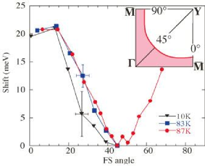
Figure 26: Momentum dependence of the gap estimated from the leading-edge shift in samples with $T_{c}$’s of 87K (slightly overdoped), 83K (UD) and 10K (UD), measured at 14K. For the sake of comparison between samples we made vertical offsets so that the shift at $45^{\circ}$ is zero; the offsets are $-3$meV for the 83K and $+2$meV for the 10K sample. The inset shows the Brillouin zone with the large Fermi surface.

6.3 Fermi Arcs

The $T$-dependence and anisotropy of the pseudogap was investigated in more detail in Ref. Nature98 motivated by the following question. Normal metallic systems are characterized by a Fermi surface, and optimally doped cuprates are no different despite the absence of sharp quasiparticles (see Section 4). On the underdoped side of the phase diagram, however, how does the opening of pseudogap affect the locus of low lying excitations in ${\bf k}$-space?

In Fig. 27 we show ARPES spectra for an UD 83K sample at three k points on the Fermi surface for various temperatures. The superconducting gap, as estimated by the position of the sample leading edge midpoint at low $T$, is seen to decrease as one moves from point a near $(\pi,0)$ to b to c, closer to the diagonal $(0,0)\to(\pi,\pi)$ direction, consistent with a $d_{x^{2}-y^{2}}$ order parameter. At each k point the quasiparticle peak disappears above $T_{c}$ as $T$ increases, with the pseudogap persisting well above $T_{c}$, as noted earlier.

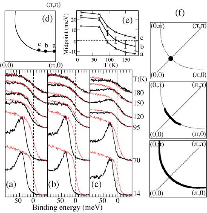
Figure 27: (a,b,c): Spectra taken at three ${\bf k}$ points in the $Y$ quadrant of the zone (shown in (d)) for an 83K underdoped Bi2212 sample at various temperatures (solid curves). The dotted curves are reference spectra from polycrystalline Pt (in electrical contact with the sample) used to determine the chemical potential (zero binding energy). Note the closing of the spectral gap at different $T$ for different ${\bf k}$’s, which is also apparent in the plot (e) of the midpoint of the leading edge of the spectra as a function of $T$. Panels (f) show a schematic illustration of the temperature evolution of the Fermi surface in underdoped cuprates. The d-wave node below $T_{c}$ (top panel) becomes a gapless arc above $T_{c}$ (middle panel) which expands with increasing $T$ to form the full Fermi surface at $T^{*}$ (bottom panel).

The striking feature which is apparent from Fig. 27 is that the pseudogap at different k points closes at different temperatures, with larger gaps persisting to higher $T$’s. At point a, near $(\pi,0)$, there is a pseudogap at all $T$’s below 180K, at which the Bi2212 leading edge matches that of Pt. As discussed above, this defines $T^{*}$ above which the the largest pseudogap has vanished within the resolution of our experiment, and a closed contour of gapless excitations – a Fermi surface – is obtained. The surprise is that if we move along this Fermi surface to point b the sample leading edge matches Pt at 120K, which is smaller than $T^{*}$. Continuing to point c, about halfway to the diagonal direction, we find that the Bi2212 and Pt leading edges match at an even lower temperature of 95K. In addition, spectra measured on the same sample along the Fermi contour near the $(0,0)\to(\pi,\pi)$ line shows no gap at any $T$ (even below $T_{c}$) consistent with $d_{x^{2}-y^{2}}$ anisotropy.

One simple way to quantify the behavior of the gap is to plot the midpoint of the leading edge of the spectrum; see Fig. 27(e). We note that a leading edge midpoint at a negative binding energy, particularly for k point c, indicates the formation of a peak in the spectral function at $\omega=0$ at high $T$. Further, we will say that the pseudogap has closed at a k point when the midpoint equals zero energy, in accordance with the discussion above. A clearer way of determining this will be presented below when we discuss the symmetrization method, but the results will be the same.

From Fig. 27, we find that the pseudogap closes at point a at a $T$ above 180K, at point b at 120 K, and at point c just below 95 K. If we now view these data as a function of decreasing $T$, the picture of Fig. 27(f) clearly emerges. With decreasing $T$, the pseudogap first opens up near $(\pi,0)$ and progressively gaps out larger portions of the Fermi contour. Thus one obtains gapless arcs which shrink as $T$ is lowered, eventually leading to the four point nodes of the $d$-wave SC gap. The existence of such arcs is apparent from the first ARPES work on the pseudogap MARSHALL , where it was noted that the Fermi contours in the pseudogap phase did not extend all the way to the zone boundary (see Fig. 28).

[width=.4]marshf4.epsf

Figure 28: Fermi level crossings from two Bi2212 samples of differing oxygen content. The entire zone can be reconstructed by fourfold rotation about (0,0) (from Ref. MARSHALL ).

Whether the arcs shrink to a point precisely at $T_{c}$ or below $T_{c}$ is not clear from the existing data. As discussed in the preceding Section, we do believe that arcs do not survive deep into the SC state where there is point node at $T\ll T_{c}$ in clean samples, as also evidenced by the linear $T$ drop in the superfluid density at low $T$.

We next turn to a powerful visualization aid that makes these results very transparent. This is the symmetrization method introduced in Ref. Nature98 , which effectively eliminates the Fermi function $f$ from ARPES data and permits us to focus directly on the spectral function $A$. Given ARPES data described byNK $I(\omega)=\sum_{\bf k}I_{0}f(\omega)A({\bf k},\omega)$ with the sum over a small momentum window about the Fermi momentum ${\bf k}_{F}$, we can generate the symmetrized spectrum $I(\omega)+I(-\omega)$. Making the reasonable assumption of particle-hole (p-h) symmetry for a small range of $\omega$ and $\epsilon_{\bf k}$, we have $A(\epsilon_{\bf k},\omega)=A(-\epsilon_{\bf k},-\omega)$ for $|\omega|,|\epsilon|$ less than few tens of meV. It then follows, using the identity $f(-\omega)=1-f(\omega)$, that $I(\omega)+I(-\omega)=\sum_{\bf k}I_{0}A({\bf k},\omega)$ which is true even after convolution with a (symmetric) energy resolution function; for details see the appendix of Ref. mesot01 . The symmetrized spectrum coincides with the raw data for $\omega\leq-2.2T_{eff}$, where $4.4T_{eff}$ is the 10%-90% width of the Pt leading edge, which includes the effects of both temperature and resolution. Non-trivial information is obtained for the range $|\omega|\leq 2.2T_{eff}$, which is then the scale on which p-h symmetry has to be valid. We have extensively checked this method, and studied in detail the errors introduced by incorrect determination of the chemical potential or of ${\bf k}_{F}$ (which lead to spurious narrow features in the symmetrized spectra), and the effect of the small ($1^{\circ}$ radius) k-window of the experiment (which was found to be small).

[width=.6]symmetryzed.epsf

Figure 29: Symmetrized spectra corresponding to the raw spectra (a,b,c) of Fig. 27. The gap closing in the raw spectrum of Fig. 27 corresponds to when the pseudogap depression disappears in the symmetrized spectrum. Note the appearance of a spectral peak at higher temperatures in c.

In Fig. 29 we show symmetrized data for the UD 83K underdoped sample corresponding to the raw data of Fig. 27. To emphasize that the symmetry is put in by hand, we show the $\omega>0$ curve as a dotted line. At k point a near $(\pi,0)$ the sharp quasiparticle peak disappears above $T_{c}$ but a strong pseudogap suppression, on the same scale as the superconducting gap, persists all the way up to 180K ($T^{*}$). Moving to panels b and c in Fig. 29 we again see pseudogap depressions on the scale of the superconducting gaps at those points, however the pseudogap fills up at lower temperatures: 120K at b and 95K at c. In panel c, moreover, a spectral peak at zero energy emerges as $T$ is raised. All of the conclusions drawn from the raw data in Fig. 27 are immediately obvious from the simple symmetrization analysis of Fig. 29.

There are many important issues related to these results that will be taken up in Section 7.3 where we describe modeling the electron self-energy in the pseudogap state. We will discuss there the remarkable $T$-dependent lineshape changes and the $T$-dependence of the gap itself. Here we simply note that, without any detailed modeling, the dataNature98 clearly show qualitative differences in the $T$-dependence at different ${\bf k}$-points. Near the $(\pi,0)$ point the gap goes away with increasing temperature with the spectral weight filling-in, but no perceptible change in the gap scale with $T$. On the other hand, at ${\bf k}_{F}$ points halfway to the node, one sees a suppression of the gap scale with increasing temperature.

We conclude this discussion with a brief mention of the implications of our results. We believe that the unusual $T$-dependence of the pseudogap anisotropy will be a very important input in reconciling the different crossovers seen in the pseudogap regime by different probes. The point here is that each experiment is measuring a k-sum weighted with a different set of k-dependent matrix elements or kinematical factors (e.g., Fermi velocity). For instance, quantities which involve the Fermi velocity, like dc resistivity above $T_{c}$ and the penetration depth below $T_{c}$ (superfluid density), should be sensitive to the region near the zone diagonal, and would thus be affected by the behavior we see at k point c. Other types of measurements (e.g. specific heat and tunneling) are more “zone-averaged” and will have significant contributions from k points a and b as well, thus they should see a more pronounced pseudogap effect. Interestingly, other data we have indicate that the region in the Brillouin zone where behavior like k point c is seen shrinks as the doping is reduced, and thus appears to be correlated with the loss of superfluid densityUEMURA . Further, we speculate that the disconnected Fermi arcs should have a profound influence on magnetotransport given the lack of a continuous Fermi contour in momentum space.

6.4 Evolution of the Fermi Surface with Doping

We now discuss the doping dependence of the normal state Fermi surface on the underdoped side of the phase diagram. The first issue to face up to is: can the Fermi arcs described above be a manifestation of a Fermi surface with small closed contours centered about $(\pi/2,\pi/2)$? Such hole-pockets enclosing $x$ holes (per planar Cu) are suggested by some theories of lightly doped Mott insulators LEE as alternatives to the large Fermi surfaces containing $(1+x)$ holes which would be consistent with the Luttinger counting.

The $T$-dependence of the arcs is by itself evidence against their being part of a pocket Fermi surface. Nevertheless, if there were such small hole pockets then one should observe two features in the ARPES data: a closure of the Fermi arc on the other side of $(\pi/2,\pi/2)$, which would be clear evidence for a “shadow band”-like dispersion ($(\pi,\pi)$-foldback of the main band) in the UD samples. In a variety of UD samples we have carefully searched for both these features and found no evidence for either DING_97 . However this is a tricky issue, given the very broad spectra and possible materials problems in the highly UD samples. Nevertheless, given the available evidence, the gapless arcs that we observe Nature98 are simply an intermediate state in the smooth evolution of $d$-wave nodes into a full Fermi surface. This smooth evolution was carefully checked on an UD 83K sample where a dense mapping was done in k space at $T=90$K, revealing only a small Fermi arc just above $T_{c}$.

[width=.8]MinGapLocus.epsf

Figure 30: (a) Midpoint shifts (dots) and widths (diamonds) for an UD 83K sample at a photon energy of 22 eV at 90K for a cut shown by the open dots in (b). (b) Fermi surface at 160K (solid triangles) and minimum gap locus at 90K (solid dots). Notice that the two surfaces coincide within error bars. The error bars represent uncertainties of Fermi crossings as well as possible sample misalignment. The solid curve is a rigid band estimate of the Fermi surface.

The other issue related to the Fermi surface is: what is its doping dependence above $T^{*}$ where the pseudogap effects are absent. While one can easily compare the near optimal and lightly UD Fermi surfaces, the rapid rise of $T^{*}$ with underdoping does not permit us to address this question. However, one can study the “minimum gap locus” in any gapped state, in close analogy with the manner in which this was defined in the SC state; see Section 5.

There is also a more fundamental reason to study the “minimum gap locus” in the pseudogap regime. One wants to know whether the pseudogap is “tied” to the Fermi surface, or if it has some other characteristic momentum Q (unrelated to ${\bf k}_{f}$). In Fig. 30(a) DING_97 we follow the dispersion of an UD 83K sample in the pseudogap regime. Moving perpendicular to the (expected) Fermi surface from occupied to unoccupied states, one finds that that the dispersion first approaches the chemical potential and then recedes away from it. This locates a ${\bf k}$-point on the minimum gap locus. For a lightly UD sample we find in Fig. 30(b) that this locus in the pseudogap regime coincides, within experimental error bars, with the Fermi surface determined above $T^{*}$ where there is no pseudogap. The pseudogap is thus tied to the Fermi surface in the same way the SC gap is, and is in contrast with, say, charge or spin density waves, which are tied to other characteristic Q vectors.

In the more heavily underdoped samples, it is not possible to compare the minimum gap locus in the pseudogap state with the Fermi surface above $T^{*}$, or the minimum gap locus below $T_{c}$, since the latter two are not measurable with $T^{*}$ too high and $T_{c}$ too low. Nevertheless, if one assumes, by continuity, that the minimum gap locus in the pseudogap state gives information about the Fermi surface that got gapped out, then even for an highly UD sample one finds a large underlying Fermi surface, satisfying the Luttinger count of $(1+x)$ holes per planar Cu DING_97 as shown in Fig. 31.

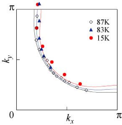
Figure 31: Fermi surfaces of the 87K, 83K, and 15K samples. All surfaces enclose a large area consistent with the Luttinger count (see text). The solid lines are tight binding estimates of the Fermi surface at 18%, 13%, and 6% doping assuming rigid band behavior.

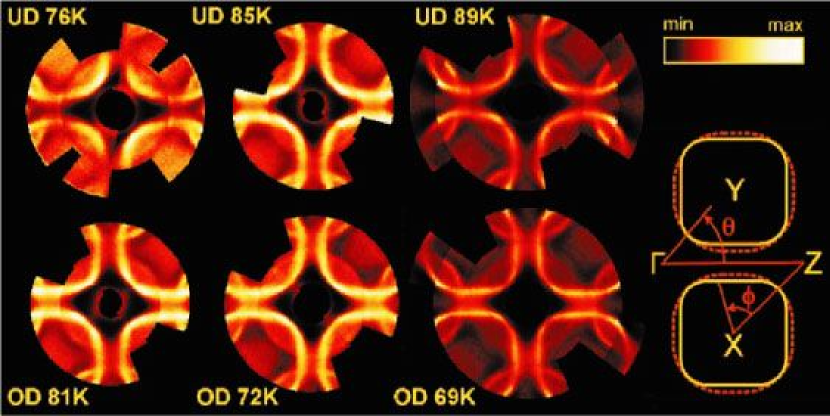
Figure 32: Basal plane projection of the normal-state (300 K) Fermi surface of Bi(Pb)-2212 from high-resolution ARPES. The $E_{F}$ intensity (normalized to the signal at $\omega$ = 0.3 eV) is shown in color. The $T_{c}$ of each sample is indicated. The raw data cover half of the colored area of each map and have been rotated by 180 around the $\Gamma$ point to give a better k-space overview. The line dividing raw and rotated data runs almost vertically for the UD76K map and from top left to bottom right in all other maps. The sketch shows the Fermi surface for the OD69K data set as yellow barrel-like shapes defined by joining the maxima of fits to the normalized $E_{F}$ MDCs. (from Ref. KORDYUK )

The same conclusion has been recently reached by the Dresden groupKORDYUK . Fig. 32 reproduces their Fermi energy intensity maps as a function of doping, where a large Fermi surface (plus its shadow band image) is always visible. They argue, though, that the volume is not quite 1+x, and they attribute this difference to the presence of bilayer splitting.

6.5 Low Energy vs High Energy Pseudogaps

In all of the preceding discussion we have focussed on the “low energy” or leading-edge pseudogap. It is important to point out that the phrase pseudogap is (somewhat confusingly) also used to describe a higher energy feature, which we call the “high energy pseudogap”.

The presence of a high energy pseudogap was evident in the first ARPES work on the pseudogap, reproduced in Fig. 33 MARSHALL . As the doping is reduced from optimal doped, a gap opens up in a region around the $(\pi,0)$ points of the zone. The energy of this gap is significantly higher than the leading edge gap emphasized in later work LOESSER ; DING_NATURE . The resulting dispersion of this high energy feature looks reminiscent of what is expected for a spin density wave gap. As the doping is further reduced, an energy gap then opens up along the $(\pi,\pi)$ direction, and the material becomes truly insulating.

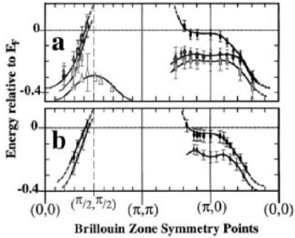
Figure 33: (a),(b) Map peak centroids vs k for Bi₂Sr₂Ca_1-xDy_xCu₂O_8+δ thin films and deoxygenated Bi₂Sr₂CaCu₂O_8+δ bulk samples, respectively, with various hole doping levels. (a) Filled oval, 1% Dy near optimal doping with T_c = 85 K; gray diamond, 10% Dy underdoped with T_c = 65 K; gray rectangular, 17.5% Dy underdoped with T_c = 25 K; triangle, 50% Dy insulator. (b) Filled oval, 600 air annealed slightly overdoped with T_c = 85 K; gray diamond, 550 argon annealed underdoped with T_c = 67 K (from Ref.MARSHALL ).

[width=.5]HighPseudo.epsf

Figure 34: Spectra at the $(\pi,0)$ point for an UD 89K sample at various temperatures compared with the low temperature (15K) spectrum. The position of the high energy feature is marked by an arrow.

In Fig. 34 JC99 we show the temperature dependence of the $(\pi,0)$ spectrum for an UD 89K sample. Note that there is no coherent quasiparticle peak until the system is cooled below $T_{c}$, with only a broad incoherent spectrum observed for all $T>T_{c}$. The leading edge pseudogap which develops below $T^{*}$ is difficult to see on the energy scale of this figure; the midpoint shift at 135 K is 3 meV. However, a higher energy feature can easily be identified by a change in slope of the spectra as function of binding energy; this is also very clear in the data of Fig. 47 of Section 7.6. At the highest temperature $T=247$K this feature is just due to the Fermi function cutoff, but in the pseudogap regime, this feature actually represents the onset of loss of spectral weight on a high energy scale, and hence may be called the “high energy pseudogap”. It can also be seen from Fig. 34 that the energy scale of this feature is very similar to that of the well-known $(\pi,0)$-hump of the peak-dip-hump structure seen in the SC state. This connection will be discussed in detail in Section 7.6 where we also argue that the high energy pseudogap and the hump have similar dispersions JC99 .

6.6 Origin of the Pseudogap?

We conclude with a summary of ARPES results on the pseudogap and a brief discussion of its theoretical understanding.

As described above, the low-energy (leading edge) pseudogap has the following characteristics.

1. The magnitude of the pseudogap near $(\pi,0)$, i.e., the scale of which there is suppression of low energy spectral weight above $T_{c}$, is the same as the maximum SC gap at low temperatures. Further both have the same doping dependence.

2. There is a crossover temperature scale $T^{*}$ above which the full Fermi surface of gapless excitations is recovered. The pseudogap near $(\pi,0)$ appears below $T^{*}$.

3. The normal state pseudogap evolves smoothly through $T_{c}$ into the SC gap as a function of decreasing temperature.

4. The pseudogap is strongly anisotropic with ${\bf k}$-dependence which resembles that of the $d$-wave SC gap. The anisotropy of the pseudogap seems to be $T$-dependent leading to the formation of disconnected Fermi arcs below $T^{*}$.

5. The pseudogap is “tied” to the Fermi surface, i.e., the minimum gap locus in the pseudogap regime coincides with the Fermi surface above $T^{*}$ and the minimum gap locus deep in the SC state, at least in those samples where all three loci can be measured.

The simplest theoretical explanation of the pseudogap, qualitatively consistent with the ARPES observations, is that it arises to due pairing fluctuations above $T_{c}$ RANDERIA ; MR_VARENNA . The SC gap increases with underdoping while $T_{c}$ decreases. Thus in the underdoped regime $T_{c}$ is not controlled by the destruction of the pairing amplitude, as in conventional BCS theory, but rather by fluctuations of the phase EMERY of the order parameter leading to the Uemura scaling $T_{c}\sim\rho_{s}$ UEMURA . Even though SC order is destroyed at $T_{c}$, the local pairing amplitude survives above $T_{c}$ giving rise to the pseudogap features. A natural mechanism for such a pseudogap coming from spin pairing in a doped Mott insulator exists within the RVB framework RVB , with possibility of additional chiral current fluctuations RVB2 .

More recently the pairing origin of the pseudogap has been challenged. Some experiments TALLON have been argued to suggest a non-pairing explanation with a competition between the pseudogap and the SC gap. A specific realization of this scenario is the staggered flux or d-density wave mechanism DDW in which $T^{*}$ is actually a phase transition below which both time-reversal and translational invariance are broken. A more subtle phase transition with only broken time-reversal has also been proposed VARMA as the origin of the pseudogap.

Although a qualitative understanding of some of the characteristics of the pseudogap within the non-pairing scenarios is not clear at this time, these theories make sharp predictions about broken symmetries below $T^{*}$ which can be tested. A very recent ARPES study KAMINSKY of circular dichroism finds evidence in favor of broken time reversal, thus casting some doubt on the pairing fluctuation ideas. The last word has clearly not been said on this subject, either theoretically or experimentally, and the origin of the pseudogap remains one of the most important open questions in the field of high $T_{c}$ superconductors.

7 Photoemission Lineshapes and the Electron Self-Energy

Under certain conditions, which were discussed in Section 2, ARPES measures the occupied part of the single particle spectral function, $A({\bf k},\omega)f(\omega)$, with $A=ImG/\pi$ where $G$ is the Greens function. The latter can be expressed as $G^{-1}=\omega-\epsilon_{\bf k}-\Sigma({\bf k},\omega)$ where $\epsilon_{\bf k}$ is the single-particle energy (defined by the kinetic energy and single-particle potential energy terms of the Hamiltonian) and $\Sigma$ is the Dyson self-energy (i.e., everything else). Often, this form is associated with a perturbative expansion used to estimate $\Sigma$, but of course the expression is itself tautological. The purpose of writing $G$ in this form is that it isolates all many-body effects in the function $\Sigma$. An advatange of ARPES is that one has the possibility of extracting $\Sigma$ directly from the data, allowing comparison to various microscopic predictions for $\Sigma$.

One of the more trivial examples of this is when one fits ARPES data to determine the superconducting gap, $\Delta$. For instance, the work described in Section 5 DING95 used a broadened form of BCS theory to fit the leading edge of the spectra. This is equivalent to $\Sigma=-i\Gamma+\Delta_{\bf k}^{2}/(\omega+\epsilon_{\bf k}+i\Gamma)$, $\Gamma=0$ describing standard BCS theory. The advantage of this procedure is the actual gap function, $\Delta$, is extracted from the data, rather than ill defined quantities, such as the often utilized leading edge shift (midpoint of the leading edge) which is not the same as $\Delta$ because of lifetime and resolution effects. When this is done, a $\Delta_{k}$ is obtained which has rather spectacular agreement with that expected for a d-wave order parameter. Although ARPES contains no phase information of the order parameter, the linear behavior of $\Delta_{k}$ along the Fermi surface near the gap zero (node) implies a sign change. Morevoer, ARPES has the additional advantage of determining the shape of $\Delta_{k}$ in the Brillouin zone, which gives important information on the spatial range of the pairing interaction MESOT , as also discussed in Section 5.

Even when fitting data at low temperatures including energy and momentum resolution, a non-zero $\Gamma$ is always needed. The origin of this residual $\Gamma$ is still debated. It is larger than what is expected based on impurity scattering, and certainly larger than that implied by various conductivity probes (thermal, microwave, and infrared). Although the transport scattering rate is different from $Im\Sigma$ (and in particular, only Umklapp processes contribute to electrical conductivity), the discrepancy is still large enough to be noticable, even when taking into account the fact that in the simple approximation being employed here, $\Gamma$ represents some average of $Im\Sigma$ over a frequency range of order $\Delta$.

Although it has been suggested that the residual $\Gamma$ is due to surface inhomogeneity effects (in particular, a distribution of $\Delta$ due to local oxygen inhomogeneities Pan ), a more likely possibility is that it is the same effect which is seen in normal metals like $TiTe_{2}$. In the latter case, it was convincingly argued that this was the expected final state lifetime contamination effect when attempting to extract $\Sigma$ from ARPES spectra TiTe2 . Although the latter is expected to vanish in the pure 2D limit, even small 3D effects can lead to a noticable effect, since final state lifetimes are large. For instance, in simple models, its contribution to $\Gamma$ is of order $(v_{c}^{i}/v_{c}^{f})\Gamma_{f}$, where $v_{c}^{i}$ is the c-axis velocity of the initial state, $v_{c}^{f}$ that of the final state, and $\Gamma_{f}$ is the final state lifetime SMITH . Since $\Gamma_{f}$ is typically of order 1 eV, then a velocity ratio of only 0.01 is sufficient to cause a residual $\Gamma$ of 10 meV.

With this as an introduction, in this section, we desire to take a more serious look at the issue of extracting $\Sigma$ from the data. The most commonly employed strategy is to come up with some model for $\Sigma$, and then see how well it fits the data, as illustrated by the simple example above. We will discuss this approach in more detail later. We start, though, with discussing an alternate approach which we have recently advocated.

7.1 Self-Energy Extraction

Let us first assume we know $A$. Given that, we can easily obtain $\Sigma$. A Kramers-Kronig transform of $A$ will give us the real part of $G$

$$ReG(\omega)=P\int_{-\infty}^{+\infty}d\omega^{\prime}\frac{A(\omega^{\prime})}{\omega^{\prime}-\omega}$$ (17)

where $P$ denotes the principal part of the integral. Knowing now both $ImG$ and $ReG$, then $\Sigma$ can be directly read off from the definition of $G$.

$$Im\Sigma=\frac{ImG}{(ReG)^{2}+(ImG)^{2}}$$ (18)

$$Re\Sigma=\omega-\epsilon-\frac{ReG}{(ReG)^{2}+(ImG)^{2}}$$ (19)

To obtain $ReG$ using Eq. 17, we need to know $A$ for all energies. From ARPES, though, we only know the product of $A$ and $f$. (While unoccupied states can be studied by inverse photoemission, its resolution at present is too poor to be useful for our purposes). This is not a limitation if an occupied ${\bf k}$-state is being analyzed and one can either ignore the unoccupied weight or use a simple extrapolation for it (except that only $Re\Sigma+\epsilon$ is determined). On the other hand, one is usually interested in $k$ vectors near the Fermi surface. Therefore a key assumption will have to be made. We can implement our procedure if we make the assumption of particle-hole symmetry, $A(\epsilon_{\bf k},\omega)=A(-\epsilon_{\bf k},-\omega)$, within the small ${\bf k}$-window centered at ${\bf k}_{F}$. Then, $A$ is obtained by exploiting the identity $A(\epsilon_{\bf k},\omega)f(\omega)+A(-\epsilon_{\bf k},-\omega)f(-\omega)=A(\epsilon_{\bf k},\omega)$, which holds even in the presence of the energy resolution convolution. Note, this can only be invoked at ${\bf k}_{F}$, and was used previously to remove the Fermi function from ARPES data Nature98 , where it was denoted as the symmetrization procedure (note that the “symmetrized” data will correspond to the raw data for $\omega<\sim-2.2kT$). Although the particle-hole symmetry assumption is reasonable for small $|\omega|$ where it can be tested in the normal state by seeing whether the “symmetrized” spectrum has a maximum at the Fermi energy ($E_{F}$), it will almost certainly fail for sufficiently large $\omega>0$. Nevertheless, since we only expect to derive $\Sigma$ for $\omega<0$, then the unoccupied spectral weight will affect the result only in two ways. The first is through the sum rule $\int d\omega A(\omega)=1$ which must be used to eliminate the intensity prefactor of the ARPES photocurrent. From Eq. 19, we see that violation of the sum rule will simply rescale $Im\Sigma$, but not $Re\Sigma$ due to the $\omega-\epsilon$ factor. Our normalization, though, is equivalent to assuming $n_{k_{F}}$=0.5, and thus does not involve “symmetrized” data. The second influence comes from the Kramers-Kronig transformation in Eq. 17, which is a bigger problem. Fortunately, the contribution from large $\omega^{\prime}>0$, for which our assumption is least valid, is suppressed by $1/(\omega^{\prime}-\omega)$. Further, for ${\bf k}_{F}$, $\epsilon_{\bf k}$=0 and thus $Re\Sigma$ is not plagued by an unknown constant.

When using real data, it is sometimes desirable to filter the noise out of the data, as well as to deconvolve the energy resolution, before employing the above procedure. These details can be found in Ref. Mike99 . Moreover, it is assumed that any “background” contribution (see Section 2) has been subtracted from the data as well.

[width=.5]fig1.epsf

Figure 35: (a) Symmetrized spectrum for overdoped Bi2212 ($T_{c}$=87K) at $T$=14K at $(\pi,0)$ with (dotted line) and without (solid line) energy resolution deconvolution. The resulting $Im\Sigma$ and $Re\Sigma$ are shown in (b) and (c). The dashed line in (c) determines the condition $Re\Sigma=\omega$.

In Fig. 35a, we show $T$=14K symmetrized data for a $T_{c}$=87K Bi2212 overdoped sample at the $(\pi,0)$ point Mike99 . We note the important differences in this superconducting state spectrum, compared with the normal state one (which can be fit by a simple Lorentzian), due to the opening of the superconducting gap, with the appearance of a sharp quasiparticle peak displaced from $E_{F}$ by the superconducting gap, followed by a spectral dip, then by a “hump” at higher binding energies. The resulting $\Sigma$ is shown in Fig. 35b and c. At high binding energies, one obtains a constant $Im\Sigma$ with a very large value ($\sim$ 300 meV). Near the spectral dip, $Im\Sigma$ has a small peak followed by a sharp drop.

Despite this sharp drop below 70 meV, $Im\Sigma$ remains quite large at low frequencies. Then, below 20 meV, there is a narrow spike in $Im\Sigma$. This is the imaginary part of the BCS self-energy, $\Delta^{2}/(\omega+i0^{+})$, which kills the normal state pole at $\omega$=0. The resulting 1/$\omega$ divergence of the real part $Re\Sigma$, which creates new poles at $\pm\Delta$=32meV, is easily seen in Fig. 35c. This is followed by a strong peak in $Re\Sigma$ near the spectral dip energy, which follows from the Kramers-Kronig transformation of the sharp drop in $Im\Sigma$. The strong peak in $Re\Sigma$ explains why the low energy peak in $A$ is so narrow despite the large value of $Im\Sigma$. The halfwidth of the spectral peak is given by $\Gamma=zIm\Sigma$ where $z^{-1}=1-\partial Re\Sigma/\partial\omega$ ($z$ is the quasiparticle residue). In the vicinity of the spectral peak, $z^{-1}$ is large ($\sim$9), giving a $\Gamma$ of $\sim$14 meV. We note, though, that $\Gamma$ is still quite sizeable, and thus the peak is not resolution limited, as discussed above.

[width=.5]fig2.epsf

Figure 36: (a) Symmetrized spectrum for underdoped Bi2212 ($T_{c}$=85K) at $T$=95K (pseudogap phase) at the $(\pi,0)-(\pi,\pi)$ Fermi crossing with (dotted line) and without (solid line) energy resolution deconvolution. The resulting $Im\Sigma$ and $Re\Sigma$ are shown in (b) and (c). The dashed line in (c) determines the condition $Re\Sigma=\omega$.

We can contrast this result with that obtained in the pseudogap phase. In Fig. 36a, we show $T$=95K symmetrized data from a $T_{c}$=85K underdoped Bi2212 sample at the $(\pi,0)-(\pi,\pi)$ Fermi crossing. One again sees (Fig. 36b) a peak in $Im\Sigma$ at $\omega$=0, but it is broadened relative to that of the superconducting state, and the corresponding divergence of $Re\Sigma$ (Fig. 36c) is smeared out. Such behavior would be consistent with replacing the BCS self-energy $\Delta^{2}/(\omega+i0^{+})$ by $\Delta^{2}/(\omega+i\Gamma_{0})$, and can be motivated by considering the presence of pair fluctuations above $T_{c}$, as will be discussed further below. Note from Fig. 36 that although the equation $\omega-Re\Sigma(\omega)=0$ is still satisfied at $|\omega|\sim\Delta$, $zIm\Sigma$ is so large that the spectral peak is strongly broadened in contrast to the sharp peak seen below $T_{c}$. Actually, to a good approximation, the spectral function is essentially the inverse of $Im\Sigma$ in the range $|\omega|<\sim 2\Delta$. We can also contrast this case with data taken above $T^{*}$, the temperature at which the pseudogap “disappears”. In that case, the spectrum is featureless, and the peak in $Im\Sigma$ is strongly broadened. As the doping increases, this peak in $Im\Sigma$ disappears. Further doping causes a depression in $Im\Sigma$ to develop around $\omega=0$, indicating a crossover to more Fermi liquid like behavior.

7.2 Temperature Dependence of $\Sigma$

We now turn to the rather controversial issue of how the spectrum at $(\pi,0)$ varies as a function of temperature, that is, how one interpolates between Figs. 35 and 36.

[width=.5]fig3.epsf

Figure 37: Temperature dependence of ARPES data at $(\pi,0)$ for a $T_{c}$=90K Bi2212 sample. The vertical dotted lines mark the spectral dip energy and the chemical potential.

In Fig. 37, we show data taken for an optimal doped ($T_{c}$=90K) Bi2212 sample Mike01 . The leading edge of the spectral peak is determined by the superconducting gap, whose energy stays fairly fixed in temperature, and persists above $T_{c}$ (the pseudogap). On the trailing edge, one sees a spectral dip, whose energy also remains fixed in temperature, and becomes filled in above $T_{c}$ due to broadening of the trailing edge of the peak.

[width=.7]fig4.epsf

Figure 38: Temperature dependence of (a) $Im\Sigma$ and (b) $Re\Sigma$ derived from the data of Fig. 37.

In Fig. 38a, $Im\Sigma$ is plotted for various temperatures. At low temperatures and energies, it is again characterized by a peak centered at zero energy due to the superconducting energy gap, and a “normal” part which can be treated as a constant plus an $\omega^{2}$ term. A maximum in $Im\Sigma$ occurs near the energy of the spectral dip. Beyond this, $Im\Sigma$ has a large, nearly frequency independent, value. As the temperature is raised, the zero energy peak broadens, the constant term increases, and the $\omega^{2}$ term goes away.

In Fig. 38b, the quantity $\omega-Re\Sigma$ is plotted. At low temperatures and energies, there is a $1/\omega$ term due to the energy gap, and a “normal” part which is linear in $\omega$. As expected, the zero crossing is near the location of the spectral peak. Beyond this, there is a minimum near the specral dip energy, then the data are approximately linear again, but with a smaller slope than near the zero crossing. As the temperature is raised, the gap (1/$\omega$) term broadens out and the low energy linear in $\omega$ term decreases, paralleling the behavior discussed above for $Im\Sigma$.

From Figs. 37 and 38, we see that rather than the spectral peak decreasing in weight with increasing temperature, it disappears by broadening strongly in energy. This can be seen directly by inspecting Fig. 38, in that as the temperature increases, $Im\Sigma$ (Fig. 38a) in the vicinity of the peak increases in magnitude with $T$, and $z^{-1}$ (roughly the slope in Fig. 38b near the zero crossing) decreases with $T$. In fact, it is the strong $T$ variation of $Im\Sigma$ and $z^{-1}$, and the fact that they operate in concert, which is responsible for the rapid variation in the effective width of the spectral peak with $T$.

The above analysis is important in that it shows how coherence is lost in the system. It is apparent from Figs. 37 and 38 that once a temperature is reached where the spectral peak is no longer discernable in the data, the difference in behavior of the self-energy between low energies and high energies is lost. That is, once the spectral dip is filled in, the low and high energy behaviors have merged, and the sharp peak and broad hump at low temperature is simply replaced by a single broad peak (with a leading edge gap due to the pseudogap). This is consistent with the spectral peak simply losing its integrity as the temperature is raised. The analysis does not support a picture of a well defined quasiparticle peak whose weight simply disappears upon heating, as has been suggested by other authors FENG_00 .

7.3 Modeling $\Sigma$

This behavior can be further quantified by fitting the self-energy for binding energies smaller than the dip energy to that expected for a superfluid Fermi liquid, and exploring the temperature dependence of the resulting parameters. The reader can find this analysis in Ref. Mike01 . Rather, we will discuss here a simpler analysis we performed where we contrasted the temperature dependence of overdoped and underdoped samples Phen98 . In this case, we chose to look at data at the $(\pi,0)-(\pi,\pi)$ Fermi crossing (antinode). The dip/hump structure is considerably weaker here than at the $(\pi,0)$ point, allowing us to concentrate on more general aspects of the spectra.

We begin with the overdoped sample, where there is no strong pseudogap effect. The simplest self-energy which can describe the low energy data at all $T$ is

$$\Sigma({\bf k},\omega)=-i\Gamma_{1}+\Delta^{2}/[(\omega+i0^{+})+\epsilon({\bf k})].$$ (20)

Here $\Gamma_{1}$ is a single-particle scattering rate taken, for simplicity, to be an $\omega$-independent constant. It is effectively an average of the (actual $\omega$-dependent) $\Sigma^{\prime\prime}$ over the frequency range of the fit. (In Ref. Mike01 , we generalized this to a constant plus an $\omega^{2}$ term, and included the resulting linear $\omega$ contribution to $\Sigma^{\prime}$). The second term is the BCS self-energy discussed previously.

[width=.7]fig5.epsf

Figure 39: Symmetrized data for (a) a $T_{c}$=82K overdoped sample and (b) a $T_{c}$=83K underdoped sample at the $(\pi,0)-(\pi,\pi)$ Fermi crossing at five temperatures, compared to the model fits described in the text.

In Fig. 39a, we show symmetrized data for an overdoped $T_{c}$=82K sample at the antinode together with the fits obtained as follows Phen98 . Using Eq. 20, we calculate the spectral function

$$\pi A({\bf k},\omega)=\Sigma^{\prime\prime}({\bf k},\omega)/\left[(\omega-\epsilon_{\bf k}-\Sigma^{\prime}({\bf k},\omega))^{2}+\Sigma^{\prime\prime}({\bf k},\omega)^{2}\right],$$ (21)

convolve it with the experimental resolution, and fit to symmetrized data. The fit is restricted to a range of $\pm$45 meV given the small gap in the overdoped case and the sharpness of the quasiparticle peaks below $T_{c}$. We find that Eq. 20 describes the low energy data quite well.

[width=.7]fig6.epsf

Figure 40: $\Delta$ (open circles), $\Gamma_{1}$ (solid circles), and $\Gamma_{0}$ (solid squares) versus $T$ at the $(\pi,0)-(\pi,\pi)$ Fermi crossing for (a) a $T_{c}$=82K overdoped sample and (b) a $T_{c}$=83K underdoped sample. The dashed line marks $T_{c}$. The error bars for $\Delta$ are based on a 10% increase in the RMS error of the fits.

The $T$-variation of the fit parameters $\Delta$ and $\Gamma_{1}$ are shown in Fig. 40a. $\Delta(T)$ decreases with $T$, and although small at $T_{c}$, it only vanishes above $T_{c}$, indicating the possibility of a weak pseudogap. This effect is sample dependent, in that several overdoped samples we have looked at, the gap vanishes closer to $T_{c}$. We caution that the error bars shown in Fig. 40a are based on the RMS error of the fits, but do not take into account experimental errors in $\mu$ and ${\bf k}_{F}$.

$\Gamma_{1}(T)$ is found to be relatively $T$-independent in the normal state. Below $T_{c}$, we see that $\Gamma_{1}$ decreases very rapidly, and can be perfectly fit to the form $a+bT^{6}$. This rapid drop in linewidth leading to sharp quasiparticle peaks at low $T$, which can be seen directly in the ARPES data, is consistent with microwave and thermal conductivity measurements, and implies that electron-electron interactions are responsible for $\Gamma_{1}$. Note the clear break in $\Gamma_{1}$ at $T_{c}$, despite the fact $\Delta$ has not quite vanished. We have seen similar behavior to that described above for a variety of overdoped samples at several k points.

We next turn to the more interesting underdoped case. We find that near $(\pi,0)$ the self-energy (20) cannot give an adequate description of the data, in that it does not properly describe the pseudogap and its unusual “filling in” above $T_{c}$. Theoretically, we cannot have a divergence in $\Sigma({\bf k}_{F},\omega=0)$ in a state without broken symmetry. A simple modification of the BCS self-energy rectifies both these problems:

$$\Sigma({\bf k},\omega)=-i\Gamma_{1}+\Delta^{2}/[\omega+\epsilon({\bf k})+i\Gamma_{0}].$$ (22)

The new term $\Gamma_{0}(T)$ should be viewed as the inverse pair lifetime. The theoretical motivation for Eq. 22 is given in Ref. Phen98 . We stress that this three parameter form is again a minimal representation of the pseudogap self-energy. Since it is not obviously a unique representation, it is very important to see what one learns from the fits.

In Fig. 39b, we show symmetrized data at the antinode for a $T_{c}$=83K underdoped sample. Below $T_{c}$ we see quasiparticle peaks. Above $T_{c}$ these peaks disappear but there is still a large suppression of spectral weight around $\omega$=0. As $T$ is raised further, the pseudogap fills in (rather than closing) leading to a flat spectrum at a temperature of $T^{*}$ (200K). The self-energy, Eq. 22, gives a good fit to the data. These fits were done below $T_{c}$ over a larger energy range ($\pm$75 meV) than in the overdoped case because of the larger gap. The range above $T_{c}$ was increased to $\pm$85 meV so as to properly describe the pseudogap depression.

In Fig. 40b, we show the $T$-dependence of the fit parameters. We find a number of surprises. First, $\Delta$ is independent of $T$ within error bars. Similar behavior has been inferred from specific heat and tunneling data. This $T$-independence is in contrast to the behavior of the overdoped 82K sample with almost identical $T_{c}$ at the same k point. In addition, for the underdoped sample, the gap evolves smoothly through $T_{c}$.

The single-particle scattering rate $\Gamma_{1}(T)$ for the underdoped sample is found to be qualitatively similar to the overdoped case. It is consistent with being $T$-independent above $T_{c}$, but with a value over twice as large as the overdoped case (allowing $\Gamma_{1}$ to vary above $T_{c}$ does not improve the RMS error of the fits). Second, we see the same rapid decrease in $\Gamma_{1}$ below $T_{c}$ as in the overdoped case. Note again the clear break at $T_{c}$.

The most interesting result is $\Gamma_{0}(T)$. We find $\Gamma_{0}=0$ below $T_{c}$ and proportional to $T-T_{c}$ above. This behavior is robust, and is seen in all the fits that we have tried. Moreover, a non-zero $\Gamma_{0}$ is needed above $T_{c}$ to obtain a proper fit to the data (its effect cannot be reproduced by varying the other parameters). The fact that this $T$-dependence is exactly what one expects of an inverse pair lifetime is a non-trivial check on the validity of the physics underlying Eq. 22. Further, we observe from Fig. 40 that $T^{*}$ corresponds to where $\Delta(T)\sim\Gamma_{0}(T)$. This condition can be understood from the small $\omega$ expansion of Eq. 22.

[width=.7]fig7.epsf

Figure 41: (a) Symmetrized data for a $T_{c}$=77K underdoped sample for three temperatures at (open circles) ${\bf k}_{F}$ point 1 in the zone inset, and at (open triangles) ${\bf k}_{F}$ point 2, compared to the model fits. (b) $\Delta(T)$ for these two k points (filled and open circles), with $T_{c}$ marked by the dashed line.

The next important question is whether the $T$-dependence at the antinode described above exists at other ${\bf k}_{F}$-points. To answer this, we have looked at $T$-dependent data for a number of underdoped samples at two different k vectors. All data at the antinode give results similar to those for the 83K sample. However at the second k-point, about halfway between the antinode and the node along the $(0,0)-(\pi,\pi)$ direction, we see quite different behavior. We demonstrate this in Fig. 41a where symmetrized data for a 77K underdoped sample are shown. For the antinode, one clearly sees the gap fill in above $T_{c}$, with little evidence for any $T$-dependence of the position of the spectral feature defining the gap edge, just as for the 83K sample. In contrast, at the second k point, the gap is clearly closing, indicating a strong $T$-dependence of $\Delta$. Similar behavior is seen in other underdoped samples with $T_{c}$ between 75 and 85K.

In Fig. 41b, we show the $T$-dependence of $\Delta$ obtained from fits (over a range of $\pm$66 meV) at the second k point for the 77K sample. $\Delta$ is found to be strongly $T$-dependent, being roughly constant below $T_{c}$, then dropping smoothly to zero above. The strong $T$-dependence of $\Delta$ makes it difficult to unambiguously determine $\Gamma_{0}$ from the fits at this k-point. On theoretical grounds, we expect that, here too, there is a non-zero $\Gamma_{0}$, and the closing of the pseudogap is again determined by $\Delta(T)\sim\Gamma_{0}(T)$, however this condition is satified by the rapid drop in $\Delta(T)$, rather than the rise in $\Gamma_{0}(T)$. For completeness, we also show $\Delta(T)$ for this sample at the antinode, which has a similar behavior to that of the 83K sample.

We see that these results give further evidence for the unusual k-dependences first noted in Ref. Nature98 . Strong pairing correlations are seen over a very wide $T$-range near $(\pi,0)$, but these effects are less pronounced and persist over a smaller $T$-range as one moves closer to the zone diagonal. This is clearly tied to the strong k-dependence of the effective interaction and the unusual (anomalously broad and non-dispersive) nature of electronic states near $(\pi,0)$.

7.4 Peak/Dip/Hump - Experiment

We now turn to a detailed discussion of the peak/dip/hump lineshape. As mentioned above, a very broad normal state spectrum near the $(\pi,0)$ point of the zone evolves quite rapidly for $T<T_{c}$ into a narrow quasiparticle peak, followed at higher binding energies by a dip then a hump, the latter corresponding to where the spectrum recovers to its normal state value PDH . Similar effects are observed in tunneling spectra PDHT .

[width=.7]fig8.epsf

Figure 42: Spectra in (a) the normal state (105 K) and (b) the superconducting state (13 K) along the line $\Gamma-\bar{M}-Z$, and (c) the superconducting state (13 K) along the line $\bar{M}-Y$ for an overdoped ($T_{c}$=87K) Bi2212 sample. The zone is shown as an inset in (c) with the curved line representing the observed Fermi surface.

In Fig. 42, we show spectra for a $T_{c}=$87K Bi2212 sample along $\Gamma-\bar{M}-Z$, i.e., $(0,0)-(\pi,0)-(2\pi,0)$, in (a) the normal state (105 K) and (b) the superconducting state (13 K), from which we note two striking features Mike97 . First, we see that the low energy peak in the superconducting state persists over a large range in ${\bf k}$-space, even when the normal state spectra have dispersed away from the Fermi energy. Second, when the hump in the superconducting state disperses, it essentially follows that of the normal state spectrum. This is accompanied by a transfer of weight to the hump from the low frequency peak, which is fairly fixed in energy. The same phenomena are also seen along $\bar{M}$ to $Y$ (Fig. 42c). We will argue that the unusual dispersion seen in the superconducting state of Fig. 42 is closely tied to the lineshape change discussed earlier (Fig. 37).

The simplest explanation of the superconducting state spectra would be the presence of two bands (e.g., due to bilayer splitting), one responsible for the peak and the other for the hump. However, this explanation is untenable Bilayer . First, if the sharp peak were associated with a second band, then this band should also appear above $T_{c}$. But there is no evidence for it in the normal state data. Second, if the peak and hump were from two different bands, then their intensities must be governed by different matrix elements. However, we found DING_96 that the intensities of both features scaled together as the photon polarization was varied from in to out of plane, as if they were governed by a common matrix element (Section 4.5). These arguments suggest that the unusual lineshape and dispersion represent a single electronic state governed by non-trivial many-body effects, as assumed in the previous discussion (Figs. 35-38). For more overdoped materials, though, bilayer splitting should be taken into account, as discussed in Section 4.5.

Under this assumption, the data are consistent with a strong reduction of the imaginary part of the self-energy ($Im\Sigma$) at low energies in the superconducting state (Fig. 35). If the scattering is electron-electron like in nature, then $Im\Sigma$ at frequencies smaller than $\sim 3\Delta$ will be suppressed due to the opening of the superconducting gap 3Delta . On closer inspection, though, a more interesting story emerges. First, from Figs. 35 and 42, we see that the superconducting and normal state data match beyond 90 meV. From 90 meV, the dip is quickly reached at 70 meV, then one rises to the sharp peak. Notice that since the width of the peak is around 20 meV, then the change in behavior of the spectra (from hump, to dip, to the trailing edge of the peak) is occuring on the scale of the energy resolution. That means that the intrinsic dip must be quite sharp. This implies that the large $Im\Sigma$ at high energies must drop to a small value over a narrow energy interval to be consistent with the data, i.e., there is essentially a step in $Im\Sigma$. In fact, the data are not only consistent with a step in $Im\Sigma$, but the depth of the dip is such that it is best fit by a peak in $Im\Sigma$ at the dip energy, followed by a rapid drop to a small value. This behavior can again be seen from the independent analysis shown in Figs. 35 and 38.

What are the consequences of this behavior in $Im\Sigma$? If $Im\Sigma$ has a sharp drop at $\tilde{\omega}$, then by Kramers-Kronig transformation, $Re\Sigma$ will have a sharp peak at $\tilde{\omega}$ (Fig. 35). This peak can very simply explain the unusual dispersion shown in Fig. 42, as it will cause a low energy quasiparticle pole to appear even if the normal state binding energy is large. The most transparent way to appreciate this result is to note that a sharp step in $Im\Sigma$ is equivalent to the problem of an electron interacting with a sharp (dispersionless) mode, since in that case, the mode makes no contribution to $Im\Sigma$ for energies below the mode energy, and then makes a constant contribution for energies above. This problem has been treated by Engelsberg and Schrieffer EngSch , and extended to the superconducting state by Scalapino and coworkers Parks . The difference in our case is that since the effect only occurs below $T_{c}$, it is a consequence of the opening of the superconducting gap in the electronic energy spectrum, and thus of a collective origin, rather than a phonon.

[width=.4]fig9.epsf

Figure 43: Positions of the sharp peak and the broad hump in the superconducting state versus normal state peak position obtained from Fig. 42a and 42b. Solid points connected by a dashed line are the data, the dotted line represents the normal state dispersion.

To facilitate comparison to this classic work, in Fig. 43 we plot the position of the low energy peak and higher binding energy hump as a function of the energy of the single broad peak in the normal state. This plot has a striking resemblance to that predicted for electrons interacting with a sharp mode in the superconducting state, and one clearly sees the low energy pole which we associate with the peak in $Re\Sigma$. On general grounds, the flat dispersion of the low energy peak seen in Fig. 43 is a combination of two effects: (1) the peak in $Re\Sigma$, which provides an additional mass renormalization of the superconducting state relative to the normal state, and thus pushes spectral weight towards the Fermi energy, and (2) the superconducting gap, which pushes spectral weight away. This also explains the strong drop in intensity of the low energy peak as the higher binding energy hump disperses.

An important feature of the data is the dispersionless nature of the sharp peak. The mode picture discussed above would imply a dispersion of the peak from $\Delta_{k}$ to $\tilde{\omega}=\omega_{0}+\Delta_{k}$ as the normal state binding energy increases (where $\omega_{0}$ is the mode energy). However, this dispersion turns out to be weak. From the data of Fig. 35, we infer an $\omega_{0}=1.3\Delta_{max}$, $\omega_{0}$ being essentially the energy separation of the peak and dip. Since $\Delta_{k}$ is known to be of the $d_{x^{2}-y^{2}}$ form, then $\Delta_{k}$ should go to zero as we disperse towards the $\Gamma$ point. Therefore, the predicted dispersion is only from $\Delta_{max}$ to $1.3\Delta_{max}$ (32 to 42 meV).

Since the dip/hump structure is most apparent at the $(\pi,0)$ points, it is natural to assume that it has something to do with $Q=(\pi,\pi)$ scattering, as discussed by Shen and Schrieffer Shen97 . But here, we find a new effect. If one compares the data of Figs. 42b and 42c, one sees that a low energy peak also exists along $(\pi,0)-(\pi,\pi)$ for approximately the same momentum range as the one from $(\pi,0)-(0,0)$. That is, if there is a peak for momentum $p$, one also exists for momentum $p+Q$. This can be understood, since the self-energy equations for $p$ and $p+Q$ will be strongly coupled if $Q$ scattering is dominant.

7.5 Mode Model

[width=.4]fig10.epsf

Figure 44: $\alpha^{2}F$ for three models, MFL (dashed line), gapped MFL (dotted line), and gapped MFL plus mode (dotted line plus $\delta$ function). Inset: Feynman diagram for the lowest order contribution to $\Sigma$ from electron-electron scattering.

For now, though, we ignore the complication of momentum dependence. The lowest order contribution to electron-electron scattering is represented by the Feynman diagram shown in the inset of Fig. 44. In the superconducting state, each internal line will be gapped by $\Delta$. This implies that the scattering will be suppressed for $|\omega|<3\Delta$. This explains the presence of a sharp quasiparticle peak at low temperatures. What is not so obvious is whether this in addition explains the strong spectral dip. Explicit calculations show only a weak dip-like feature Little92 . To understand this in detail, we equate the bubble plus interaction lines (Fig. 44 inset) to an “$\alpha^{2}F$” as in standard strong-coupling literature. In a marginal Fermi liquid (MFL) at T=0, $\alpha^{2}F(\Omega)$ is simply a constant in $\Omega$. The effect of the gap is to force $\alpha^{2}F$ to zero for $\Omega<2\Delta$. The question then arises where the gapped weight goes. It could be distributed to higher energies, but in light of the above discussion, we might expect it to appear as a collective mode inside of the $2\Delta$ gap. For instance, if the bubble represents spin fluctuations, a sharp mode will appear if the condition $1-U\chi_{0}({\bf q},\Omega)=0$ is satisfied for $\Omega<2\Delta$. These three cases (MFL, gapped MFL, gapped MFL plus mode) are illustrated in Fig. 44.

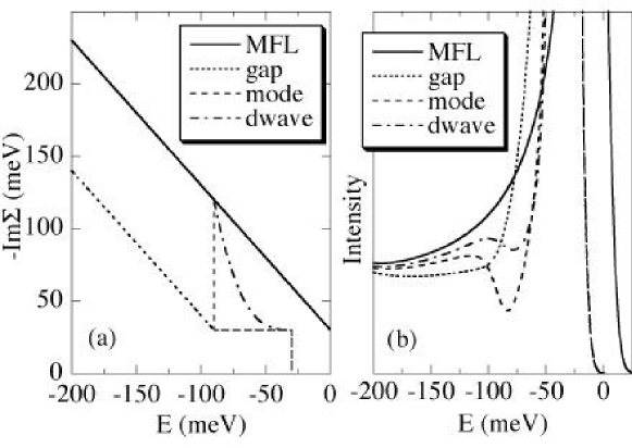
Figure 45: (a) $Im\Sigma$ for MFL (solid line), gapped MFL (dotted line), gapped MFL plus mode (dashed line), and simple d-wave model (dashed-dotted line). Parameters are $\alpha$=1, $\omega_{c}$=200meV, $\Delta$=30meV (0 for MFL), $\Omega_{0}$=2$\Delta$, and $\Gamma_{0}$=30meV. (b) Spectral functions (times a Fermi function with $T$=14K) convolved with a resolution gaussian of $\sigma$=7.5 meV for these four cases ($\epsilon$=-34meV).

$\Sigma$ is easy to obtain analytically if we ignore the complication of the superconducting density of states from the $\bf k-q$ line of Fig. 44 and just replace this by a step function at $\Delta$. The resulting $Im\Sigma$ for the gapped MFL and gapped MFL plus mode models are shown in Fig. 45a ND98 in comparison to the normal state MFL. Note that structure in $\alpha^{2}F$ at $\Omega$ appears in $\Sigma$ at $|\omega|=\Omega+\Delta$ due to the gap in the $\bf k-q$ line. Moreover, the MFL plus mode is simply the normal state MFL cut-off at $3\Delta$ (this is obtained under the assumption that all the gapped weight in $\alpha^{2}F$ shows up in the mode). In contrast, the gapped MFL decays linearly to zero at $3\Delta$.

The Nambu spectral function is given by

$$A(\omega)=\frac{1}{\pi}Im\frac{Z\omega+\epsilon}{Z^{2}(\omega^{2}-\Delta^{2})-\epsilon^{2}}$$ (23)

with (a complex) $Z(\omega)=1-\Sigma(\omega)/\omega$. These are shown in Fig. 45b and were convolved with a gaussian of $\sigma$=7.5 meV, typical of high resolution ARPES, with a constant $Im\Sigma$ ($\Gamma_{0}$) added for $|\omega|>\Delta$ to reduce the size of the quasiparticle peak. We note that there is no dip as such for the gapped MFL model, whereas the addition of the mode causes a significant dip. The latter behavior is consistent with experiment. Moreover, the mode model has the additional advantage that $Im\Sigma$ recovers back to the normal state value by $3\Delta$, which is also in agreement with experiment in that the normal and superconducting state spectra agree beyond 90 meV (Figs. 35 and 42).

We contrast this behavior with that expected for a simple d-wave model. To a first approximation, this can be obtained by replacing the step drop in $Im\Sigma$ in the MFL plus mode model with $(|\omega|-\Delta)^{3}$ for $|\omega|<3\Delta$ Quinlan96 . This is shown in Fig. 45a as well, with the resulting spectrum in Fig. 45b. Only a weak dip appears. Moreover, we have analyzed models with the exponent 3 replaced by some n and have found that n must be large to obtain a dip as strong as seen in experiment. Therefore, the upshot is that at the least, something similar to a step is required in $Im\Sigma$ to be consistent with experiment.

In principle, we could take the above MFL plus mode model and fit experiment with it. We consider a simpler model. There are several reasons for this. First, the MFL model has a number of adjustable parameters associated with it. There is the coupling constant ($\alpha$), the cut-off frequency ($\omega_{c}$), and the mode energy (which is not in general $2\Delta$). Moreover, the spectrum for $\bf k$ points near the $(\pi,0)$ point does not appear to be MFL-like in nature. We have found that the normal state Bi2212 spectrum is fit very well by a Lorentzian plus a constant background in an energy range less than $0.5$eV. This is also true for Bi2201 spectrum where the normal state can be accessed to much lower temperatures.

In the resulting Lorentzian model, the normal state $\Sigma$ is purely an imaginary constant, and $\alpha^{2}F$ is a mode at zero energy. In the superconducting state, this mode gets pushed back to some energy within $2\Delta$. This model is artificial in the sense that all the self-energy is being generated by the mode. That is why we went through the above discussion motivating the mode more properly as a rearrangement of $\alpha^{2}F$ due to the superconducting gap. In practice, though, the results are very similar to the MFL plus mode model, and has the further advantage of having the several parameters of that model collapse to just the mode strength ($\Gamma_{1}$) and mode position ($\Omega_{0}$) of the Lorentzian model. Moreover, analytic results can still be obtained for $\Sigma$ when the superconducting density of states for the $\bf k-q$ line of Fig. 44 is taken into account. The result is ND98

$$-Im\Sigma(\omega) = \Gamma_{0}N(|\omega|)+\Gamma_{1}N(|\omega|-\Omega_{0}),\;|\omega|>\Omega_{0}+\Delta$$ (24)

$$= \Gamma_{0}N(|\omega|),\;\Delta<|\omega|<\Omega_{0}+\Delta$$ (25)

$$= 0,\;|\omega|<\Delta$$ (26)

where $N(\omega)=\omega/\sqrt{\omega^{2}-\Delta^{2}}$ is the BCS density of states, and

$$\pi Re\Sigma(\omega)=\Gamma_{0}N(-\omega)\ln\left[{|-\omega+\sqrt{\omega^{2}-\Delta^{2}}|}/{\Delta}\right]$$ (27)

$$+\Gamma_{1}N(\Omega_{0}-\omega)\ln\left[{|\Omega_{0}-\omega+\sqrt{(\omega-\Omega_{0})^{2}-\Delta^{2}}|}/{\Delta}\right]$$ (28)

$$-\{\omega\rightarrow-\omega\}$$ (29)

where it has again been assumed that $\Delta$ is a real constant in frequency. An s-wave density of states has been used to obtain an analytic result. A d-wave density of states will not be that different. The advantage of an analytic result is that it is useful when having to take spectra and convolve with resolution to compare to experiment. Our results are not very sensitive to $\Gamma_{0}$, included again to damp the quasiparticle peak.

[width=.7]fig12.epsf

Figure 46: (a) $Im\Sigma$ and $ReZ$ at $(\pi,0)$ from Eqs. 26 and 29 ($\Gamma_{1}$=200meV, $\Gamma_{0}$=30meV, $\Delta$=32meV, $\Omega_{0}$=1.3$\Delta$). Comparison of the data at $(\pi,0)$ for (b) wide and (c) narrow energy scans with calculations based on Eqs. 23-29, with an added step edge background contribution.

The resulting real (Eq. 29) and imaginary (Eq. 26) parts of $\Sigma$ at $(\pi,0)$ are shown in Fig. 46a. Note the singular behaviors at $\Delta$ (peak energy) due to the $\Gamma_{0}$ term and at $\Omega_{0}+\Delta$ (dip energy) due to the $\Gamma_{1}$ term. In both cases, step drops in $Im\Sigma$ would also give singularities in $Re\Sigma$. The advantage of peaks in $Im\Sigma$ (due to the SC density of states) is that it makes the dip deeper in better agreement with experiment. In Fig. 46b and 46c, we show a comparison of the resulting spectral function (convolved with the experimental energy and momentum resolution) to experimental data at $(\pi,0)$ for both wide and narrow energy scans, where a step edge background with a gap of $\Delta$ is added to the calculated spectrum. The resulting agreement is excellent.

It is interesting to note that the mode energy we infer from the data is 41 meV, equivalent to a magnetic resonant mode energy observed in YBCO YBCO and Bi2212 BSCO by neutron scattering data at ${\bf Q}=(\pi,\pi)$. The $Q$ dependence of this mode correlates well with the observations of Fig. 42. To explore this in greater detail, we now consider the doping dependence of the peak/dip/hump structure.

7.6 Doping Dependence

[width=.7]fig13.epsf

Figure 47: Spectra along $(\pi,0)\to(\pi,\pi)$ in (a) the superconducting state (T=60K), and (b) the pseudogap state (T=100K) for an underdoped 75K sample (curves are labeled in units of $\pi/a$). The thick vertical bar indicates the position of the higher energy feature, at which the spectrum changes slope as highlighted by the intersecting straight lines.

We show data along $(\pi,0)\to(\pi,\pi)$ for an underdoped 75K sample in the superconducting state (Fig. 47a) and in the pseudogap state (Fig. 47b) JC99 . Below $T_{c}$, the sharp peak at low energy is essentially dispersionless, while the higher energy hump rapidly disperses from the $(\pi,0)$ point towards the $(\pi,0)\to(\pi,\pi)$ Fermi crossing seen above $T^{*}$. Beyond this, the intensity drops dramatically, but there is clear evidence that the hump disperses back to higher energy. In the pseudogap state, the high energy feature also shows strong dispersion, much like the hump below $T_{c}$, even though the leading edge is non-dispersive like the sharp peak in the superconducting state.

[width=.7]fig14.epsf

Figure 48: Doping dependence of the dispersion from (a) $(\pi,0)\to(\pi\pm\pi,0)$, (b) $(\pi,0)\to(\pi,\pm\pi)$, and (c) both directions, for the peak and hump in the superconducting state. U is underdoped and O is overdoped. Points were obtained by polynomial fits to the data, and are consistent with the simpler criterion used in Fig. 47.

In Fig. 48 we show the dispersion of the sharp peak and hump (below $T_{c}$), for a variety of doping levels, in the vicinity of the $(\pi,0)$ point along the two principal axes. The sharp peak at low energies is seen to be essentially non-dispersive along both directions for all doping levels, while the hump shows very interesting dispersion. Along $(\pi,0)\to(0,0)$ (Fig. 48a), the hump exhibits a maximum, with an eventual dispersion away from the Fermi energy, becoming rapidly equivalent to the binding energy of the broad peak in the normal state as one moves away from the region near $(\pi,0)$. In the orthogonal direction (Fig. 48b), since the hump initially disperses towards the $(\pi,0)\to(\pi,\pi)$ Fermi crossing, which is known to be a weak function of doping, one obtains the rather dramatic effect that the dispersion becomes stronger with underdoping. We also note that there is an energy separation between the peak and the hump due to the spectral dip. In essence, the hump disperses towards the spectral dip, but cannot cross it, with its weight dropping strongly as the dip energy is approached. Beyond this point, one sees evidence of the dispersion bending back to higher binding energy for more underdoped samples.

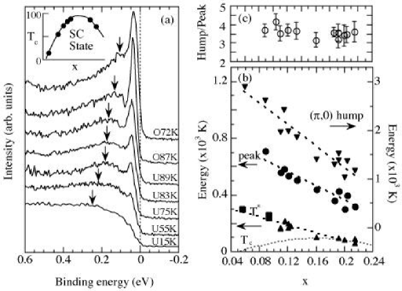
Figure 49: Dependence of energy scale on carrier density: (a) Doping dependence of the spectra (T=15K) at the $(\pi,0)$ point. The inset shows $T_{c}$ vs. doping. (b) Doping dependence of $T^{*}$, and the peak and hump binding energies in the superconducting state along with their ratio (c), as a function of doping, $x$. The empirical relation between $T_{c}$ and $x$ is given by $T_{c}/T_{c}^{max}=1-82.6(x-0.16)^{2}$ with $T_{c}^{max}$=95K. For $T^{*}$, solid squares represent lower bounds.

Fig. 49a shows the evolution of the low temperature spectra at the $(\pi,0)$ point as a function of doping. The sharp quasiparticle peak moves to higher energy, indicating that the gap increases with underdoping (although this is difficult to see on the scale of Fig. 49a). We see that the hump moves rapidly to higher energy with underdoping. These trends can be seen very clearly in Fig. 49b, where the energy of the peak and hump are shown as a function of doping for a large number of samples. Finally, we observe that the quasiparticle peak loses spectral weight with increasing underdoping, as expected for a doped Mott insulator; in addition the hump also loses spectral weight though less rapidly.

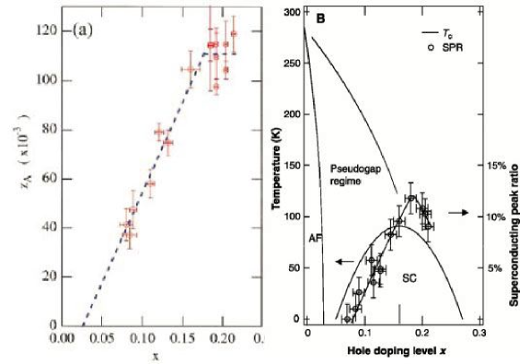
Figure 50: (a) Doping dependence of the low-T (14 K) coherent weight (z_A). The dashed line is a guideline showing that z_A increases linearly on the underdoped side, and tapers off on the overdoped side. (from Ref. DING_00 ) (b) The doping dependence of the superconducting peak ratio (SPR) is plotted over a typical Bi2212 phase diagram. The solid line is a guide to the eye. Horizontal error bars denote uncertainty in determining the doping level ($\pm$0.01); vertical error bars denote uncertainty in determining the SPR ($\pm$1.5%). AF, antiferromagnetic regime; SC, superconducting regime. (from Ref. FENG_00 )

This effect has recently been quantified in greater detail, where it was found that the spectral weight of the peak varies linearly with doping, as reproduced in Fig. 50. FENG_00 ; DING_00 . We remark that Ding et al.DING_00 also found the unusual relation that the product of the peak weight times the peak energy is constant with doping.

The hump below $T_{c}$ is clearly related to the superconducting gap, given the weak doping dependence of the ratio between the hump and quasiparticle peak positions at $(\pi,0)$, shown in Fig. 49c. Tunneling data find this same correlation on a wide variety of high-$T_{c}$ materials whose energy gaps vary by a factor of 30 JohnZ96 .

To motivate the analysis below that firmly establishes the mode interpretation of of the peak/dip/hump spectra and its connection with neutron data, we note that the spectral dip represents a pairing induced gap in the incoherent part of the spectral function at $(\pi,0)$ occurring at an energy $\Delta+\Omega_{0}$, where $\Delta$ is the superconducting gap and $\Omega_{0}$ is the mode energy. We can estimate the mode energy from ARPES data from the energy difference between the dip ($\Delta+\Omega_{0}$) and the quasiparticle peak ($\Delta$).

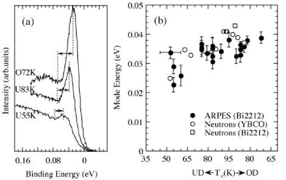
Figure 51: Doping dependence of the mode energy: (a) Spectra at $(\pi,0)$ showing the decrease in the energy separation of the peak and dip with underdoping. Peak and dip locations were obtained by independent polynomial fits and carefully checked for the effects of energy resolution. (b) Doping dependence of the collective mode energy inferred from ARPES together with that inferred from neutron data Bourges98 .

In Fig. 51b we plot the mode energy as estimated from ARPES for various doping levels as a function of $T_{c}$ and compare it with neutron measurements. We find striking agreement both in terms of the energy scale and its doping dependence Bourges98 . The same agreement, in greater detail, has been recently found using tunneling data JohnZ01 , as shown in Fig. 52. We note that the mode energy inferred from ARPES decreases with underdoping, just like the neutron data, unlike the gap energy (Fig. 49b), which increases. This can be seen directly in the raw data, shown in Fig. 51a. This is also seen from the tunneling data, where they have found that the mode energy scales with doping as 5$T_{c}$, just like the neutron resonance. An interesting point from the tunneling is that the ratio of the mode energy to the gap energy saturates to 2 in the overdoped limit, as would be expected for a collective mode sitting below a continuum with a gap of 2$\Delta$. Moreover, there is strong correlation between the temperature dependences in the ARPES and neutron data. While neutrons see a sharp mode only below $T_{c}$, a smeared out remnant persists up to $T^{*}$ Dai96 . As the sharpness of the mode is responsible for the sharp spectral dip, one then sees the correlation with ARPES where the dip disappears above $T_{c}$, but with a remnant of the hump persisting to $T^{*}$.

[width=.5]johnz.epsf

Figure 52: Measured mode energy $\Omega$ and bulk $T_{c}$ value vs. measured gap value $\Delta$ for 17 junctions over a wide doping range from UD74K to OD48K. Solid and dashed lines are quadratic fits of $\Omega$ and $T_{c}$ vs. $\Delta$. Inset shows $\Omega/\Delta$ vs. $\Delta$ (from Ref. JohnZ01 ).

An important feature of the neutron data is that the mode only exists in a narrow momentum range about $(\pi,\pi)$, and is magnetic in origin. To see a further connection with ARPES, we return to the results of Fig. 48. Note the dispersion along the two orthogonal directions are similar (Fig. 48c), unlike the dispersion inferred in the normal state. As these two directions are related by a $(\pi,\pi)$ translation ($(x,0)\equiv(0,-x);(0,-x)+(\pi,\pi)=(\pi,\pi-x)$), we see that the hump dispersion is clearly reflecting the $(\pi,\pi)$ nature of the collective mode. This dispersion is also consistent with a number of models in the literature which identify the high energy feature in the pseudogap regime as a remnant of the insulating magnet InsTh . We note, though, that the mode is due to quasiparticle pair creation and thus not just a continuation of the spin wave mode from the antiferromagnet ModeTh .

This brings up a question that is at the heart of the high $T_{c}$ problem: how can a feature which can be understood as a strong coupling effect of superconductivity, as discussed above, turn out to have a dispersion that resembles that of a magnetic insulator? The reason is that the collective mode has the same wavevector, $(\pi,\pi)$, which characterizes the magnetic order of the insulator. It is easy to demonstrate that in the limit that the mode energy goes to zero (long range order), one actually reproduces a symmetric dispersion similar to that in Fig. 48c, with the spectral gap determined by the strength of the mode KAMPF . This is in accord with the increase in the hump energy with underdoping (Fig. 49b) tracking the rise in the neutron mode intensity. Since the hump scales with the superconducting gap, the obvious implication is that the mode is intimately connected with pairing, a conclusion which can also be made by relating the mode to the superconducting condensation energy Dai99 . That is, high $T_{c}$ superconductivity is likely due to the same magnetic correlations which characterize the insulator and give rise to the mode.

7.7 Dispersion Kink of Nodal Quasiparticles

So far, our discussion has largely been centered on behavior near the $(\pi,0)$ point of the zone. We now turn to consideration of other ${\bf k}$ vectors.

Remarkably, we find that the effects discussed above are manifest even on the zone diagonal where the gap vanishes, with significant changes in both the spectral lineshape and dispersion below $T_{c}$, relative to the normal state where the nodal points exhibit quantum critical scaling Valla99 . Specifically, below $T_{c}$ a kink in the dispersion develops along the diagonal at a finite energy ($\sim$70 meV) Kink ; Adam01 . This is accompanied, as required by Kramers-Krönig relations, by a reduction in the linewidth leading to well-defined quasiparticles Adam00 . As one moves away from the node, the renormalization increases, and the kink in dispersion along the diagonal smoothly evolves into the spectral dip, with the same characteristic energy scale throughout the zone.

In Fig. 53a, we plot the dispersion of the spectral peak above $T_{c}$ obtained from constant ${\bf k}$ scans (energy distribution curves or EDCs), and the peak in momentum obtained from constant $\omega$ scans (momentum distribution curves or MDCs) Valla99 from data for a $T_{c}$=90K sample along the $(\pi,\pi)$ direction Adam01 . We find that the EDC and MDC peak dispersions are very different, a consequence of the $\omega$ dependence of $\Sigma$.

To understand this, we start by noting that since $\epsilon_{{\bf k}}\simeq v_{F}^{0}(k-k_{F})$, then from Eq. 8 the MDC at fixed $\omega$ is a Lorentzian centered at $k=k_{F}+\left[\omega-\Sigma^{\prime}(\omega)\right]/v_{F}^{0}$, with a width (HWHM) $W_{M}=|\Sigma^{\prime\prime}(\omega)|/v_{F}^{0}$, provided (i) $\Sigma$ is essentially independent of $k$ normal to the Fermi surface, and (ii) the dipole matrix elements do not vary significantly with $k$ over the range of interest. That these two conditions are fulfilled can be seen by the nearly Lorentzian MDC lineshape observed in ARPES Valla99 .

On the other hand, in general, the EDC at fixed ${\bf k}$ has a non-Lorentzian lineshape reflecting the non-trivial $\omega$-dependence of $\Sigma$, in addition to the Fermi cutoff at low energies. Thus the EDC peak is not given by $\omega-v_{F}^{0}(k-k_{F})-\Sigma^{\prime}(\omega)=0$ but also involves $\Sigma^{\prime\prime}$, unlike the MDC peak. Further, if the EDC peak is sharp enough, making a Taylor expansion we find that its width (HWHM) is given by $W_{E}\simeq|\Sigma^{\prime\prime}(E_{k})|/[1-\partial\Sigma^{\prime}/\partial\omega|_{E_{k}}]$, where $E_{k}$ is the peak position.

We see that it is much simpler to interpret the MDC peak positions, and thus focus on the change in the MDC dispersion going from the normal (N) to the superconducting (SC) state shown in Fig. 53b. The striking feature of Fig. 53b is the development of a kink in the dispersion below $T_{c}$. At fixed $\omega$ let the dispersion change from $k_{N}$ to $k_{SC}$. Using $v_{F}^{0}(k_{N}-k_{SC})=\Sigma_{SC}^{\prime}(\omega)-\Sigma_{N}^{\prime}(\omega)$, we directly obtain the change in real part of $\Sigma$ plotted in Fig. 53c. The Kramers-Krönig transformation of $\Sigma_{SC}^{\prime}-\Sigma_{N}^{\prime}$ then yields $\Sigma_{N}^{\prime\prime}-\Sigma_{SC}^{\prime\prime}$, plotted in Fig. 53d, which shows that $|\Sigma_{SC}^{\prime\prime}|$ is smaller than $|\Sigma_{N}^{\prime\prime}|$ at low energies.

[width=.7]fig17.epsf

Figure 53: ARPES data along the $(\pi,\pi)$ direction at $h\nu$=28eV. (a) EDC dispersion in the normal state compared to the MDC dispersion. The EDCs are shown in Fig. 54d. (b) MDC dispersions in the superconducting state (T=40K) and normal state (T=115K). (c) change in MDC dispersion from (b). (d) Kramers-Krönig transform of (c).

We compare these results in Fig. 54a with the $W_{M}=|\Sigma^{\prime\prime}|/v_{F}^{0}$ estimated directly from the MDC Lorentzian linewidths. The normal state curve was obtained from a linear fit to the corresponding MDC width data points in Fig. 54a, and then the data from Fig. 53d was added to it to generate the low temperature curve. We are thus able to make a quantitative connection between the appearance of a kink in the (MDC) dispersion below $T_{c}$ and a drop in the low energy scattering rate in the superconducting state relative to the normal state, which leads to the appearance of quasiparticles below $T_{c}$ Adam00 . We emphasize that we have estimated these $T$-dependent changes in the complex self-energy without making fits to the EDC lineshape, thus avoiding the problem of modeling the $\omega$ dependence of $\Sigma$ and the extrinsic background.

In Fig. 54b, we plot the EDC width obtained as explained in Ref. Adam00 from Fig. 54d. As an interesting exercise, we present in Fig. 54c the ratio of this EDC width to the MDC width of Fig. 54a (dotted lines), and compare it to the renormalized MDC velocities, $1/v\equiv dk/d\omega$, obtained directly by numerical differentiation of Fig. 53b (solid lines). We note that only for a sufficiently narrow EDC lineshape is the ratio $W_{E}/W_{M}\simeq v_{F}^{0}/[1-\partial\Sigma^{\prime}/\partial\omega]=v_{F}$. Interestingly, only in the superconducting state below the kink energy do these two quantities agree, which implies that only in this case does one have a Fermi liquid.

Similar kinks in the dispersion have been seen by ARPES in normal metals due to the electron-phonon interaction Baer99 . Phonons cannot be the cause here, since the kink disappears above $T_{c}$. Rather, this effect is suggestive of coupling to an electronic collective excitation which only appears below $T_{c}$. Recently, this view has been challenged by Lanzara et al.Shen01 , and we discuss this work at the end of this subsection.

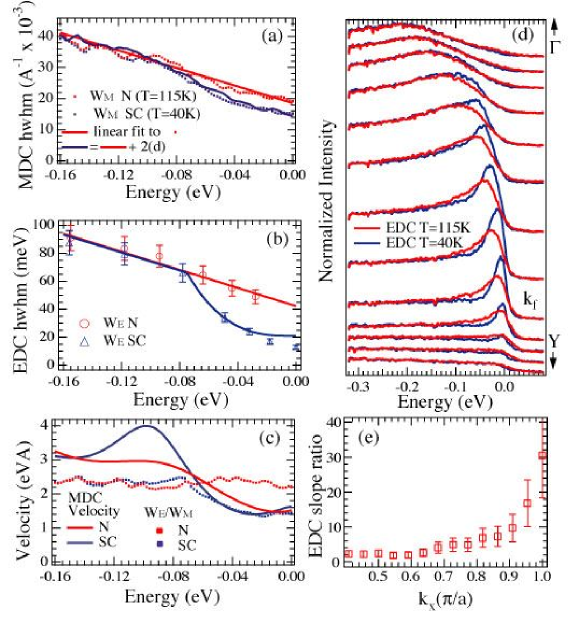
Figure 54: (a) Comparison of change in $\Sigma^{\prime\prime}$ obtained directly from the MDC widths (HWHM) to the one obtained from the dispersion in Fig. 53d by using the Kramers-Krönig transform. (b) HWHM width obtained from EDCs shown in (d). Lines marked by fit are linear in normal state and linear/cubic in superconducting state. The data in (b) fall below the fits at low energies because of the Fermi cut-off of the EDCs. (c) Renormalized MDC velocity obtained from differentiating Fig. 53b (solid lines), compared to the ratio $W_{E}/W_{M}$ from (a) and (b). (e) Ratio of EDC dispersion slopes above and below the kink energy at various points along the Fermi surface (from middle panels of Fig. 55).

We now study how the lineshape and dispersion evolve as we move along the Fermi surface. An analysis similar to the above is possible, but more complicated due to the presence of an energy gap MDC01 . We will thus confine ourselves here to a general description of the data. In Fig. 55, we plot raw intensities for a series of cuts parallel to the $MY$ direction (normal state in left panels, superconducting state in middle panels). We start from the bottom row that corresponds to a cut close to the node and reveals the same kink described above. As we move towards $(\pi,0)$, the dispersion kink (middle panels) becomes more pronounced and at around $k_{x}$=0.55 develops into a break separating the faster dispersing high energy part of the spectrum from the slower dispersing low energy part. This break leads to the appearance of two features in the EDCs, shown in the right panels of Fig. 55. Further towards $(\pi,0)$, the low energy feature, the quasiparticle peak, becomes almost dispersionless. At the $(\pi,0)$ point, this break effect becomes the most pronounced, giving rise to the peak/dip/hump in the EDC. We note that there is a continuous evolution in the zone from kink to break, and these features all occur at exactly the same energy.

[width=.7]fig19.epsf

Figure 55: Left panels: Log of normal state ($h\nu$=22eV, T=140K) ARPES intensity along selected cuts parallel to $MY$. EDC peak positions are indicated by crosses. Middle panels: Log of superconducting state (T=40K) intensity at the same cuts as for left panels. Crosses indicate positions of broad high energy peaks, dots sharp low energy peaks. Right panels: EDCs at locations marked by the vertical lines in the middle panels.

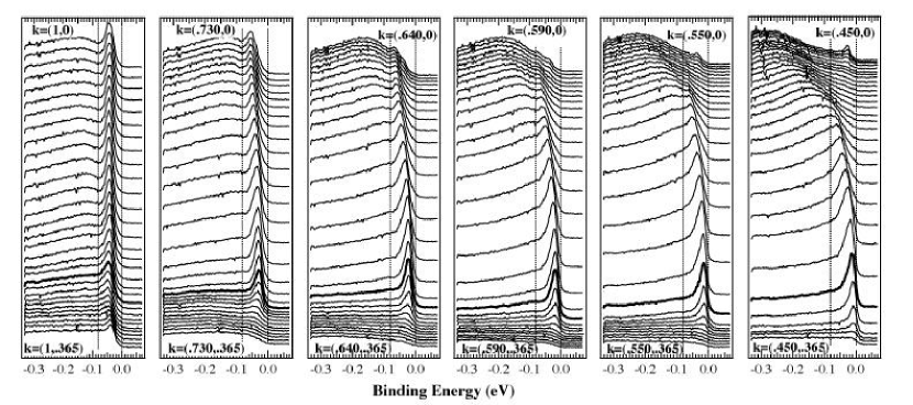
Figure 56: ARPES intensity (T=40K) along selected cuts from Fig. 55. The thick lined curves correspond approximately to ${\bf k}_{F}$. Vertical lines are at 0 and -80 meV.

The above evolution is suggestive of the self-energy becoming stronger as the $(\pi,0)$ point is approached. This can be quantified from the observed change in the dispersion. In Fig. 54e we plot the ratio of the EDC dispersion slope above and below the kink energy at various points along the Fermi surface obtained from middle panels of Fig. 55. Near the node, this ratio is around 2, but becomes large near the $(\pi,0)$ point because of the nearly dispersionless quasiparticle peak. A different behavior was inferred in Ref. Shen01 , but in their case, the cuts near $(\pi,0)$ were perpendicular to ours, and thus not normal to the Fermi surface.

The lineshape also indicates that the self-energy is larger near $(\pi,0)$, as is evident in Fig. 56. Along the diagonal, there is a gentle reduction in $\Sigma^{\prime\prime}$ at low energies, as shown in Fig. 54a and b, with an onset at the dispersion kink energy scale. In contrast, near the $(\pi,0)$ point there must be a very rapid change in $\Sigma^{\prime\prime}$ in order to produce a spectral dip, as discussed above. Despite these differences, it is important to note that these changes take place throughout the zone at the same characteristic energy scale (vertical line in Fig. 56).

As also discussed above, the $(\pi,0)$ ARPES spectra can be naturally explained in terms of the interaction of the electron with a collective mode of electronic origin which only exists below $T_{c}$. It was further speculated that this mode was the neutron resonance. Here we have shown that dispersion and lineshape anomalies have a continuous evolution throughout the zone and are characterized by a single energy scale. This leads us to suggest that the same electron-mode interaction determines the superconducting lineshape and dispersion at all points in the zone, including the nodal direction. In essence, there is a suppression of the low energy scattering rate below the finite energy of the mode. Of course, since the neutron mode is characterized by a $(\pi,\pi)$ wavevector, one would expect its effect on the lineshape to be much stronger at points in the zone which are spanned by $(\pi,\pi)$, as observed here.

A similar conclusion has been reached by Johnson et al. PJ01 , where they find that the kink energy scales with doping like the neutron resonance (Fig. 57a), and that the temperature dependence of $\Sigma^{\prime}$ tracks that of the resonance intensity (Fig. 57b). Moreover, they find that $\Sigma^{\prime}$ increases with underdoping (Fig. 57a), much like that extracted from the peak/dip/hump lineshape at $(\pi,0)$.

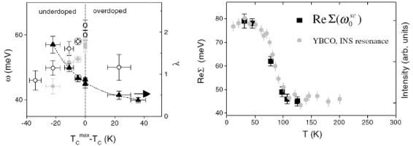
Figure 57: Left panel: Plot of $\omega_{0}$, the energy of the maximum value of Re$\Sigma$ in the superconducting state (open circles), and $\omega_{0}^{SC}$ (gray circles), the energy of the maximum in difference between the superconducting and normal state values plotted as a function of T_c referenced to the maximum $T^{max}_{c}$ ($\equiv$ 91 K). The coupling constant $\lambda$ (black triangles) is referenced to the right-hand scale. Right panel: Temperature dependence of Re$\Sigma(\omega^{SC}_{0})$ from the nodal line for the UD69K sample (black squares) compared with the temperature dependence of the intensity of the resonance mode observed in inelastic neutron scattering studies of underdoped YBa₂Cu₃O_6+x, $T_{c}$ = 74 K (gray circles) (adapted from Ref.PJ01 ).

Detailed calculations which take into account the momentum dependence of the neutron resonance give an extremely good description of the experimental data EN00 . These results can be understood by studying the Feynman diagram of Fig. 44. The key point is that the neutron resonance has a finite width in momentum space, corresponding to a short correlation length of order 2 lattice constants. Because of this, there is now an internal sum over momentum in the diagram, which will be dominated by the flat regions of the fermionic dispersion around the $(\pi,0)$ points. This means that structure in the electron self-energy will occur at an energy of $\Delta_{max}+\Omega_{res}$, independent of external momentum. This explains why the energy scale is invariant throughout the zone. On the other hand, as the external momentum is swept, the momentum dependence of the neutron form factor is probed. Since the latter peaks at $Q=(\pi,\pi)$, then the magnitude of the self-energy will be maximal at $(\pi,0)$, since these points are connected by $Q$, and minimum at the node. This explains why the peak/dip/hump effect first weakens into a “break” effect and then into a dispersion kink as the node is approached. These calculations have been recently extended to incorporate bilayer splitting effects EN02 , and are able to explain a number of unusual lineshape and dispersion features present in data on heavily overdoped Bi2212 BILAY1 ; BILAY2 ; BILAY3 ; BILAY4

As mentioned above, this picture has been challenged by Lanzara et al.Shen01 . These authors claim that the kink is still present above $T_{c}$, except it is smeared in energy. Moreover, they find that a kink is present in a large variety of cuprates, including Bi2201 and LSCO, with an energy which is material and doping independent, as shown in Fig. 58. They argue that all of these observations are in support of a phonon interpretation of the kink.

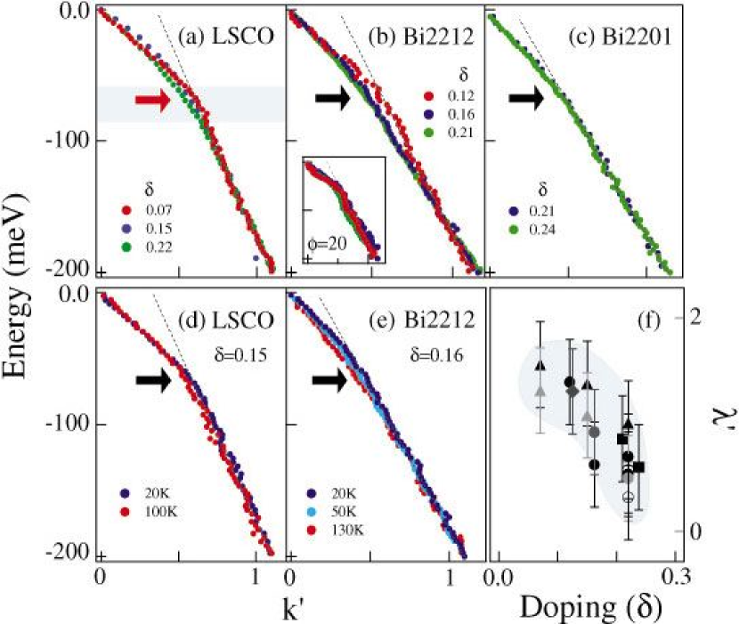
Figure 58: Ubiquity of a sudden change (‘kink’) in the dispersion. Top panels are plots of the dispersion (derived from the momentum distribution curves) along $(0,0)-(\pi,\pi)$ (except panel b inset, which is off this line) versus the rescaled momentum k’ for different samples and at different doping levels. a-c, Doping ($\delta$) dependence of LSCO (at 20 K; a), Bi2212 (superconducting state, 20 K; b), and Bi2201 (normal state, 30 K; c). Dotted lines are guides to the eye. The kink position in a is compared with the phonon energy at $q=(\pi,0)$ (thick red arrow) and the phonon width and dispersion (shaded area) from neutron data. The doping was determined from the $T_{c}$ versus doping universal curve. Inset in b, dispersions off the (0, 0) - $(\pi,\pi)$ direction, showing also a sharpening of the kink on moving away from the nodal direction. The black arrows indicate the position of the kink in the dispersions. d,e, Temperature dependence of the dispersions for LSCO (d, optimally doped) and Bi2212 (e, optimally doped). f, Doping dependence of $\lambda$ along the (0, 0) - $(\pi,\pi)$ direction as a function of doping. Data are shown for LSCO (filled triangles) and NdLSCO (1/8 doping; filled diamonds), Bi2201 (filled squares) and Bi2212 (filled circles in the first Brillouin zone, and unfilled circles in the second zone). The different shadings represent data obtained in different experimental runs. Blue area is a guide to the eye. (adapted from Ref.Shen01 ).

Although initially attractive, there are some problems with this scenario. First, in regards to the kink above $T_{c}$, it has been claimed by Johnson et al.PJ01 that the “kink” above $T_{c}$ is simply the curvature in the dispersion one expects based on marginal Fermi liquid theory. In support of this, they argue that the maximum in the real part of $\Sigma$ is at a different energy in the normal state than in the superconducting state. Though this appears to be the case, there is indeed residual structure in the normal state self-energy at the kink energy in the optimal doped sample we have looked at. On the other hand, our normal state data actually corresponds to the pseudogap phase, and as a residual of the neutron resonance is present in the pseudogap phase, the residual “kink” above $T_{c}$ (if really there) does not rule out a magnetic intepretation. Moreover, as Johnson et al.convincingly showed (Fig. 57b), there is definitely a large component to the self-energy which follows the same order paramter like temperature variation that the neutron resonance intensity does. This observation is supported by recent work of Gromko et al.BILAY4 concerning a dispersion kink in the bonding band of heavily overdoped Bi2212 near $(\pi,0)$.

Second, in regards to constancy of the energy scale, this is indeed an interesting observation, though we note this statement contradicts that of Johnson et al.concerning the doping dependence of the kink energy mentioned above (Fig. 57). Also, even in a phonon model, the kink energy should occur at the sum of the maximum gap energy plus the phonon energy. Why the sum of these two numbers should be doping and material independent is a real puzzle (as it would be for a magnetic interpretation as well). And, why only one phonon would be relevant, despite the large number of phonons present in the cuprates, is another puzzle. Still, a phonon model for the kink has certain attractions, as discussed by Lanzara et al.Shen01 . Certainly, more work is needed to definitively resolve the controversies surrounding the origin of the dispersion kink.

7.8 Condensation Energy

We conclude this section by discussing the relation of ARPES data to the superconducting condensation energy.

We begin with the assumption that the condensation energy does not have a component due to phonons. To proceed, we assume an effective single-band Hamiltonian which involves only two particle interactions. Then, simply exploiting standard formulas for the internal energy $U=\langle H-\mu N\rangle$ ($\mu$ is the chemical potential, and $N$ the number of particles) in terms of the one-particle Green’s function, we obtain Mike00

$$U_{N}-U_{S}=$$ (31)

$$\sum_{\bf k}\int_{-\infty}^{+\infty}d\omega(\omega+\epsilon_{k})f(\omega)\left[A_{N}({\bf k},\omega)-A_{S}({\bf k},\omega)\right]$$

where the spin variable has been summed over. Here and below the subscript $N$ stands for the normal state, $S$ for the superconducting state. $A({\bf k},\omega)$ is the single-particle spectral function, $f(\omega)$ the Fermi function, and $\epsilon_{k}$ the bare energy dispersion which defines the kinetic energy part of the Hamiltonian. Note that the $\mu N$ term has been absorbed into $\omega$ and $\epsilon_{k}$, that is, these quantities are defined relative to the appropriate chemical potential, $\mu_{N}$ or $\mu_{S}$. In general, $\mu_{N}$ and $\mu_{S}$ will be different. This difference has to be taken into account, since the condensation energy is small.

The condensation energy is defined by the zero temperature limit of $U_{N}-U_{S}$ in the above expression. Note that this involves defining (or somehow extrapolating to) the normal state spectral function at $T=0$. Such an extrapolation, which we return to below, is not specific to our approach, but required in all estimates of the condensation energy. We remark that Eq. 31 yields the correct condensation energy, $N(0)\Delta^{2}/2$, for the BCS theory of superconductivity.

We also note that Eq. 31 can also be broken up into two pieces to individually yield the thermal expectation value of the kinetic energy (using $2\epsilon_{k}$ in the parentheses in front of $f(\omega)$), and that of the potential energy (using $\omega-\epsilon_{k}$ instead).

The great advantage of Eq. 31 is that it involves just the occupied part of the single particle spectral function, which is measured by ARPES. Therefore, in principle, one should be able to derive the condensation energy from such data, if an appropriate extrapolation of the normal state spectral function to T=0 can be made. On the other hand, a disadvantage is that the bare energies, $\epsilon_{k}$, are a priori unknown. Note that these are not directly obtained from the measured ARPES dispersion, which already includes many-body renormalizations. Rather, they could be determined by projecting the kinetic energy operator onto the single-band subspace.

Some of the problems associated with an analysis based on experimental data can be appreciated. First, the condensation energy is obtained by subtracting two large numbers. Therefore, normalization of the data becomes a central concern. Problems in this regard when considering $n({\bf k})$, which is the zeroth moment of the ARPES data, were discussed previously JC98 . For the first moment, these problems are further amplified due to the $\omega$ weighting in the integrand. When analyzing real data, we have found that the high energy tail contribution to the first moment is very sensitive to how the data are normalized. Different choices of normalization can even lead to changes in sign of the first moment.

Another concern concerns the ${\bf k}$ sum in Eq. 31. ARPES has ${\bf k}$-dependent matrix elements, which lead to weighting factors not present in Eq. 31. These effects can in principle be factored out by either theoretical estimates of the matrix elements Bansil99 , or by comparing data at different photon energies to obtain information on them mesot01 .

Another issue in connection with experimental data is an appropriate extrapolation of the normal state to zero temperature. Information on this can be obtained by analyzing the temperature dependence of the normal state data, remembering that the Fermi function will cause a temperature dependence of the data which should be factored out before attempting the $T=0$ extrapolation. We finally note that the temperature dependence issue is strongly coupled to the normalization problem mentioned above. In ARPES, the absolute intensity can change due to temperature dependent changes in absorbed gasses, surface doping level, and sample location. Changes of background emission with temperature is another potential problem.

Despite these concerns, we believe that with careful experimentation, many of these difficulties can be overcome, and even if an exact determination of Eq. 31 is not possible, insights into the origin of the condensation energy will certainly be forthcoming from the data. This is particularly true for ARPES, which has the advantage of being ${\bf k}$ resolved and thus giving one information on the relative contribution of different ${\bf k}$ vectors to the condensation energy.

Insights into what real data might indicate have been offered by us Mike00 in the context of the “mode” model illustrated in Fig. 46. What we found was that for parameters characteristic of optimal doped ARPES data, the superconducting condensation was driven by kinetic energy lowering, as opposed to the potential energy lowering found in BCS theory. This occurs because $n_{k}$ becomes sharper in the superconducting state than in the normal state. In essence, the normal state is a non Fermi liquid and the superconducting state is a Fermi liquid, so what occurs is that the effect of quasiparticle formation on sharpening $n_{k}$ is greater than the effect of particle-hole mixing on smearing it. The net result is a sharpening, leading to a lowering in kinetic energy. In BCS theory, the normal state is a Fermi liquid, and thus only the particle-hole mixing effect is present, leading to a net smearing of $n_{k}$ and thus an increase in the kinetic energy. The same model can be used to evaulate the optical sum rule NP02 , and what is found is a violation of the sum rule with a sign and magnitude consistent with recent optics experiments OPT . It will be of great interest to see whether these results can be confirmed directly from ARPES data, as speculated early on by Anderson And90 .

8 Acknowledgments

Much of the experimental work described in this article was done in collaboration with Hong Ding, Adam Kaminski, Helen Fretwell, Kazimierz Gofron, Joel Mesot, Stephan Rosenkranz, Tsunehiro Takeuchi, and the group of Takashi Takahashi, including Takafumi Sato and Takayoshi Yokoya. We were very fortunate to have available to us the samples from Kazuo Kadowaki, T. Mochiku, David Hinks, Prasenjit Guptasarma, Boyd Veal, Z. Z. Li, and Helene Raffy. We have also benefited from many interactions over the years with Phil Anderson, Alex Abrikosov, Jim Allen, Cliff Olson, Ole Andersen, Al Arko, Bertram Batlogg, Arun Bansil, Matthias Eschrig, Atsushi Fujimori, Peter Johnson, Bob Laughlin, Bob Schrieffer, Z. X. Shen, and Chandra Varma.

This work was supported by the National Science Foundation, Grant No. DMR 9974401 (JCC) and the U.S. Department of Energy, Office of Science, under Contract No. W-31-109-ENG-38 (JCC and MRN). MR is grateful for partial support from the Indian DST through the Swarnajayanti scheme.

References

- (1) A. Chainani, T. Yokoya, T. Kiss, S. Shin, Phys. Rev. Lett. 85, 1966 (2000).
- (2) A. Damascelli, Z.-X. Shen, Z. Hussain, Rev. Mod. Phys. (2002), cond-mat/0208504.
- (3) D.L. Lynch and C.G Olson, Photoemission studies of high-temperature superconductors (Cambridge University Press, Cambridge, UK, 1999).
- (4) S. Hüfner, Photoelectron Spectroscopy (Springer-Verlag, Berlin, 1996), and references therein.
- (5) C.N. Berglund and W.E. Spicer, Phys. Rev. 136, A1030 and A1044 (1964).
- (6) In general, the matrix element also contains a term. Above the bulk plasma frequency, the light penetrates deeply into the solid, making this term small. This “surface photoemission” has not been prominent in the many studies of the cuprates, and we will henceforth ignore it.
- (7) J. Hermanson, Solid State Comm. 22, 9 (1977).
- (8) For a review of the first five years of work on the cuprates, see Sec. 4 and 5 of Z. X. Shen and D. S. Dessau, Phys. Repts. 253, 1 (1995).
- (9) J. Mesot, M. Randeria, M. R. Norman, A. Kaminski, H.M. Fretwell, J. C. Campuzano, H. Ding, T. Takeuchi, T. Sato, T. Yokoya, T. Takahashi, I. Chong, T. Terashima, M. Takano, T. Mochiku, and K. Kadowaki, Phys. Rev. B 63, 224516 (2001).
- (10) H. Hertz, Ann. Physik 31, 983 (1887).
- (11) W. L. Schaich and N. W. Ashcroft, Phys. Rev. B 3, 2452 (1971).
- (12) C. Caroli, D. Lederer-Rozenblatt, B. Roulet, and D. Saint-James, Phys. Rev. B 8, 4552 (1973).
- (13) J. B. Pendry, Surf. Sci. 57, 679 (1976). For a review of applications of these methods to the cuprates, see: A. Bansil and M. Lindroos, J. Phys. Chem. Solids 56, 1855 (1995).
- (14) C.G. Larsson, Surface Science 152/153, 213 (1985); ibid 162, 19 (1985).
- (15) P.A.P. Lindberg, L.I. Johansson and A.N. Christensen, Surface Science 197, 353 (1987).
- (16) F.L. Hopkinson, J.B. Pendry, and D.J. Titterington, Comput. Phys. Comm. 26, 111 (1980).
- (17) A. Bansil, M. Lindroos, and J.C. Campuzano, Proc. Mater. Res. Soc. 253, 519 (1992); M. Lindroos, A. Bansil, K. Gofron, H. Ding, J.C. Campuzano, R. Liu, and B.W. Veal, Physica C 212, 347 (1993).
- (18) H.L. Edwards, J.T. Markert and A.L. de Lozanne, Phys. Rev. Lett. 69, 2967 (1992).
- (19) N. V. Smith, P. Thiry, and Y. Petroff, Phys. Rev. B 47, 15476 (1993).
- (20) See, e.g., L. Hedin and S. Lundquist, Solid State Physics 23, 1 (Academic, New York, 1969).
- (21) M. Randeria, H. Ding, J-C. Campuzano, A. Bellman, G. Jennings, T. Yokoya, T. Takahashi, H. Katayama-Yoshida, T. Mochiku, and K. Kadowaki, Phys. Rev. Lett. 74, 4951 (1995).
- (22) H. Ding, J. C. Campuzano, A. F. Bellman, T. Yokoya, M. R. Norman, M. Randeria, T. Takahashi, H. Katayama-Yoshida, T. Mochiku, K. Kadowaki, G. Jennings, Phys. Rev. Lett. 74, 2784 (1995) and 75, 1425 (E) (1995).
- (23) A. V. Federov, T. Valla, P. D. Johnson, Q. Li, G. D. Gu, N. Koshizuka, Phys. Rev. Lett. 82, 2179 (1999); T. Valla, A.V. Fedorov, P.D. Johnson, B.O. Wells, S.L. Hulbert, Q. Li, G.D. Gu, and N. Koshizuka, Science 285, 2110 (1999); T. Valla, A. V. Fedorov, P. D. Johnson, Q. Li, G. D. Gu, N. Koshizuka, Phys. Rev. Lett. 85, 828 (2000).
- (24) P.V. Bogdanov, A. Lanzara, S.A. Kellar, X.J. Zhou, E.D. Lu, W.J. Zheng, G. Gu, J.-I. Shimoyama, K. Kishio, H. Ikeda, R. Yoshizaki, Z. Hussain, and Z. X. Shen, Phys. Rev. Lett. 85, 2581 (2000).
- (25) A. Kaminski, M. Randeria, J. C. Campuzano, M. R. Norman, H. Fretwell, J. Mesot, T. Sato, T. Takahashi, and K. Kadowaki, Phys. Rev. Lett. 86, 1070 (2001).
- (26) M. R. Norman, M. Eschrig, A. Kaminski, J. C. Campuzano, Phys. Rev. B 64, 184508 (2001).
- (27) W. E. Pickett, Rev. Mod. Phys. 61, 433 (1989).
- (28) P. W. Anderson, The Theory of Superconductivity in the High- Cuprates (Princeton Univ. Pr., Princeton, 1997).
- (29) O. K. Andersen A. I. Liechtenstein, O. Jepsen, F. Paulsen, J. Phys. Chem. Solids 56, 1573 (1995).
- (30) P. W. Anderson, Science 235, 1196 (1987).
- (31) C. G. Olson, R. Liu, D. W. Lynch, R. S. List, A. J. Arko, B. W. Veal, Y. C. Chang, P. Z. Jiang, and A. P. Paulikas, Phys. Rev. B 42, 381 (1990).
- (32) The electronic structure of the insulator has been extensively studied by the Stanford group, confirming beautifully the predicted valence band maximum at , see B. O. Wells, Z.-X. Shen, A. Matsuura, D. M. King, M. A. Kastner, M. Greven, and R. J. Birgeneau, Phys. Rev. Lett. 74, 964 (1995).
- (33) A. Kaminski, J. Mesot, H. Fretwell, J. C. Campuzano, M. R. Norman, M. Randeria, H. Ding, T. Sato, T. Takahashi, T. Mochiku, K. Kadowaki, and H. Hoechst, Phys. Rev. Lett. 84, 1788 (2000).
- (34) J. C. Campuzano, G. Jennings, M. Faiz, L. Beaulaigue, B. W. Veal, J. Z. Liu, A. P. Paulikas, K. Vandervoort, H. Claus, Phys. Rev. Lett. 64, 2308 (1990).
- (35) D. M. King, Z.-X. Shen, D. S. Dessau, B. O. Wells, W. E. Spicer, A. J. Arko, D. S. Marshall, J. DiCarlo, A. G. Loeser, C. H. Park, E. R. Ratner, J. L. Peng, Z. Y. Li, R. L. Greene, Phys. Rev. Lett. 70, 3159 (1993); R. O. Anderson, R. Claessen, J. W. Allen, C. G. Olson, C. Janowitz, L. Z. Liu, J.-H. Park, M. B. Maple, Y. Dalichaouch, M. C. de Andrade, R. F. Jardim, E. A. Early, S.-J. Oh, W. P. Ellis, ibid 70, 3163 (1993); N. P. Armitage, D. H. Lu, C. Kim, A. Damascelli, K. M. Shen, F. Ronning, D. L. Feng, P. Bogdanov, Z.-X. Shen, Y. Onose, Y. Taguchi, Y. Tokura, P. K. Mang, N. Kaneko, M. Greven, ibid 87, 147003 (2001); N. P. Armitage, F. Ronning, D. H. Lu, C. Kim, A. Damascelli, K. M. Shen, D. L. Feng, H. Eisaki, Z.-X. Shen, P. K. Mang, N. Kaneko, M. Greven, Y. Onose, Y. Taguchi, Y. Tokura, ibid 88, 257001 (2002).
- (36) A. Ino, C. Kim, T. Mizokawa, Z.-X. Shen, A. Fujimori, M. Takaba, K. Tamasaku, H. Eisaki, S. Uchida, J. Phys. Soc. Japan 68, 1496 (1999); A. Ino, C. Kim, M. Nakamura, T. Mizokawa, Z.-X. Shen, A. Fujimori, T. Kakeshita, H. Eisaki, S. Uchida, Phys. Rev. B 62, 4137 (2000); A. Ino, C. Kim, M. Nakamura, T. Yoshida, T. Mizokawa, Z.-X. Shen, A. Fujimori, T. Kakeshita, H. Eisaki, S. Uchida, ibid 65, 094504 (2002); T. Yoshida, X. J. Zhou, M. Nakamura, S. A. Kellar, P. V. Bogdanov, E. D. Lu, A. Lanzara, Z. Hussain, A. Ino, T. Mizokawa, A. Fujimori, H. Eisaki, C. Kim, Z.-X. Shen, T. Kakeshita, S. Uchida, ibid, 63, 220501 (2001).
- (37) H. Ding, A. F. Bellman, J. C. Campuzano, M. Randeria, M. R. Norman, T. Yokoya, T. Takahashi, H. Katayama-Yoshida, T. Mochiku, K. Kadowaki, G. Jennings, and G. P. Brivio, Phys. Rev. Lett. 76, 1533 (1996).
- (38) M. R. Norman, M. Randeria, H. Ding, and J. C. Campuzano, Phys. Rev. B 52, 615 (1995).
- (39) R. L. Withers, J. G. Thompson, L. R. Wallenberg, J. D. Fitzgerald, J. S. Anderson, B. G. Hyde, J. Phys. C 21, 6067 (1988).
- (40) P. Aebi, J. Osterwalder, P. Schwaller, L. Schlapbach, M. Shimoda, T. Mochiku and K. Kadowaki, Phys. Rev. Lett. 72, 2757 (1994); J. Osterwalder, P. Aebi, P. Schwaller, L. Schlapbach, M. Shimoda, T. Mochiku and K. Kadowaki, Appl. Phys. A 60, 247 (1995).
- (41) A. Kampf and J. R. Schrieffer, Phys. Rev. B 42, 7967 (1990).
- (42) H. Ding, M.R. Norman, T. Yokoya, T. Takuechi, M. Randeria, J.C. Campuzano, T. Takahashi, T. Mochiku, and K. Kadowaki, Phys. Rev. Lett. 78, 2628 (1997).
- (43) A. A. Kordyuk, S. V. Borisenko, M. S. Golden, S. Legner, K. A. Nenkov, M. Knupfer, J. Fink, H. Berger, L. Forro, R. Follath, Phys. Rev. B 66, 014502 (2002).
- (44) This would allow us to understand (1) why polarization selection rules are obeyed for the mirror plane, and (2) qualitatively, why the intensities for odd and even polarizations along are comparable.
- (45) D. S. Dessau, Z. X. Shen, D. M. King, D. S. Marshall, L. W. Lombardo, P. H. Dickinson, A. G. Loeser, J. DiCarlo, C. H Park, A. Kapitulnik, and W. E. Spicer, Phys. Rev. Lett. 71, 2781 (1993).
- (46) M. R. Norman, M. Randeria, H. Ding, J. C. Campuzano, and A. F. Bellman, Phys. Rev. B 52, 15107 (1995).
- (47) T. Sato, T. Kamiyama, T. Takahashi, J. Mesot, A. Kaminski, J. C. Campuzano, H. M. Fretwell, T. Takeuchi, H. Ding, I. Chong, T. Terashima, M. Takano, Phys. Rev. B 64, 054502 (2001).
- (48) N. L. Saini, J. Avila, A. Bianconi and A. Lanzara, M. C. Asensio, S. Tajima, G. D. Gu, and N. Koshizuka, Phys. Rev. Lett. 79, 3467 (1997).
- (49) J. Mesot, M. R. Norman, H. Ding, J. C. Campuzano, Phys. Rev. Lett. 82, 2618 (1999); N. L. Saini, A. Bianconi, A. Lanzara, J. Avila, M. C. Asensio, S. Tajima, G. D. Gu, N. Koshizuka, ibid 2619 (1999).
- (50) Y.-D. Chuang, A. D. Gromko, D. S. Dessau, Y. Aiura, Y. Yamaguchi, K. Oka, A. J. Arko, J. Joyce, H. Eisaki, S. I. Uchida, K. Nakamura, and Yoichi Ando, Phys. Rev. Lett. 83, 3717 (1999).
- (51) H.M. Fretwell, A. Kaminski, J. Mesot, J. C. Campuzano, M. R. Norman, M. Randeria, T. Sato, R. Gatt, T. Takahashi, and K. Kadowaki, Phys. Rev. Lett. 84, 4449 (2000).
- (52) S. V. Borisenko, M. S. Golden, S. Legner, T. Pichler, C. Durr, M. Knupfer, J. Fink, G. Yang, S. Abell, H. Berger, Phys. Rev. Lett. 84, 4453 (2000); S. V. Borisenko, A. A. Kordyuk, S. Legner, C. Durr, M. Knupfer, M. S. Golden, J. Fink, K. Nenkov, D. Eckert, G. Yang, S. Abell, H. Berger, L. Forro, B. Liang, A. Mailouck, C. T. Lin, B. Keimer, Phys. Rev. B 64, 094514 (2001).
- (53) The data in Ref. fretwell00 is taken in the superconducting state (K) of the K sample. We note that the integration range (100 meV) employed for the intensity patterns is much larger than the gap energy scale, and the minimum gap locus (to be discussed below in Section 6) in the superconducting state is essentially identical to the normal state Fermi surface.
- (54) D.L. Feng, W.J. Zheng, K.M. Shen, D.H. Lu, F. Ronning, J.-I. Shimoyama, K. Kishio, G. Gu, D. Van der Marel, Z.-X. Shen, cond-mat/9908056.
- (55) J. C. Campuzano, H. Ding, M. R. Norman, M. Randeria, A. F. Bellman, T. Yokoya, T. Takahashi, H. Katayama-Yoshida, T. Mochiku, and K. Kadowaki, Phys. Rev. B 53, R14737 (1996).
- (56) Th. Straub, R. Claessen, P. Steiner, S. Hufner, V. Eyert, K. Friemelt and E. Bucher, Phys. Rev. B 55, 13473 (1997).
- (57) M. C. Schabel, C.-H. Park, A. Matsuura, Z.-X. Shen, D. A. Bonn, Ruixing Liang, and W. N. Hardy, Phys. Rev. B 57, 6107 (1998).
- (58) K. Gofron, J. C. Campuzano, H. Ding, C. Gu, R. Liu, B. Dabrowski, B. W. Veal, W. Cramer, G. Jennings, J. Phys. Chem. Sol. 54, 1193 (1993); K. Gofron, J. C. Campuzano, A. A. Abrikosov, M. Lindroos, A. Bansil, H. Ding, D. Koelling, B. Dabrowski, Phys. Rev. Lett. 73, 3302 (1994).
- (59) S. Massida, J. Yu, and A.J. Freeman, Physica C 152, 251 (1988); O. K. Andersen, O. Jepsen, A. I. Liechtenstein, I. I. Mazin, Phys. Rev. B 49, 4145 (1994).
- (60) S. Chakravarty, A. Sudbo, P. W. Anderson and S. Strong, Science 261, 337 (1994).
- (61) M.R. Norman, H. Ding, J.C. Campuzano, T. Takeuchi, M. Randeria, T. Yokoya, T. Takahashi, T. Mochiku, and K. Kadowaki, Phys. Rev. Lett. 79, 3506 (1997).
- (62) J. C. Campuzano, H. Ding, M. R. Norman, H. M. Fretwell, M. Randeria, A. Kaminski, J. Mesot, T. Takeuchi, T. Sato, T. Yokoya, T. Takahashi, K. Kadowaki, P. Guptasarma, D. G. Hinks, Z. Konstantinovic, Z. Z. Li, and H. Raffy, Phys. Rev. Lett. 83, 3709 (1999).
- (63) J. Zasadzinski, L. Ozyuzer, Z. Yusof, J. Chen, K. E. Gray, R. Mogilevsky, D. G. Hinks, J. L. Cobb, J. T. Markert, SPIE 2696, 338 (1996); See also J. Zasadzinski et al. (unpublished) in Fig. 1 of D. Coffey, J. Phys. Chem. Solids 54, 1369 (1993).
- (64) P. W. Anderson, Science 256, 1526 (1992).
- (65) D.L. Feng, N.P. Armitage, D.H. Lu, A. Damascelli, J.P Hu, P. Bogdanov, A. Lanzara, F. Ronning, K.M. Shen, H. Eisaki, C. Kim, and Z.-X. Shen, Phys. Rev. Lett. 86, 5550 (2001); D.L. Feng, C. Kim, H. Eisaki, D.H. Lu, A. Damascelli, K.M. Shen, F. Ronning, N. P. Armitage, N. Kaneko, M. Greven, J.-I. Shimoyama, K. Kishio, R. Yoshizaki, G.D. Gu, Z.-X. Shen, Phys. Rev. B 65, 220501 (2002).
- (66) Y. D. Chuang, A. D. Gromko, A. Fedorov, D. S. Dessau, Y. Aiura, K. Oka, Y. Ando, H. Eisaki, S. I. Uchida, Phys. Rev. Lett. 87, 117002 (2001); Y. D. Chuang, A. D. Gromko, A. Fedorov, Y. Aiura, K. Oka, Y. Ando, D. S. Dessau, cond-mat/0107002.
- (67) A. A. Kordyuk, S. V. Borisenko, T. K. Kim, K. Nenkov, M. Knupfer, M. S. Golden, J. Fink, H. Berger, R. Follath, Phys. Rev. Lett. 89, 077003 (2002).
- (68) D.L. Feng, A. Damascelli, K.M. Shen, N. Motoyama, D.H. Lu, H. Eisaki, K. Shimizu, J.-I. Shimoyama, K. Kishio, N. Kaneko, M. Greven, G.D. Gu, X.J. Zhou, C. Kim, F. Ronning, N. P. Armitage, and Z.-X. Shen, Phys. Rev. Lett. 88, 107001 (2002); D.L. Feng, H. Eisaki, K.M. Shen, A. Damascelli, C. Kim, D.H. Lu, Z.-X. Shen, K. Shimizu, J.-I. Shimoyama, K. Kishio, N. Motoyama, N. Kaneko, M. Greven, G.D. Gu, Intl. J. of Mod. Phys. 16, 1691 (2002); T. Sato, H. Matsui, S. Nishina, T. Takahashi, T. Fujii, T. Watanabe, and A. Matsuda, Phys. Rev. Lett. 89, 067005 (2002).
- (69) D. J. Van Harlingen, Rev. Mod. Phys 67, 515 (1995); C. C. Tsuei and J. R. Kirtley, ibid 72, 969 (2000).
- (70) Z. X. Shen, D. S. Dessau, B. O. Wells, D. M. King, W. E. Spicer, A. J. Arko, D. Marshall, L. W. Lombardo, A. Kapitulnik, P. Dickinson, S. Doniach, J. DiCarlo, A. G. Loeser, C. H. Park, Phys. Rev. Lett. 70, 1553 (1993).
- (71) H. Ding, M. R. Norman, J. C. Campuzano, M. Randeria, A. Bellman, T. Yokoya, T. Takahashi, T. Mochiku, and K. Kadowaki, Phys. Rev. B 54, R9678 (1996).
- (72) J.-M. Imer, F. Patthey, B. Dardel, W.-D. Schneider, Y. Baer, Y. Petroff, A. Zettl, Phys. Rev. Lett. 62, 336 (1989).
- (73) C. G. Olson, R. Liu, A.-B. Yang, D. W. Lynch, A. J. Arko, R. S. List, B. W. Veal, Y. C. Chang, P. Z. Jiang, A. P. Paulikus, Science 245, 731 (1989).
- (74) The large dispersion along , of about 60 meV within our momentum window , makes it hard to locate accurately and to map out the nodal region. To this end the we use a step size of normal to the Fermi surface and along it.
- (75) See: D. Pines and P. Monthoux, J. Phys. Chem. Solids 56, 1651 (1995) and D. J. Scalapino, Phys. Rep. 250, 329 (1995).
- (76) R. J. Kelley, J. Ma, C. Quitmann, G. Margaritondo, M. Onellion, Phys. Rev. B 50, 590 (1994).
- (77) J. M. Harris, Z.-X. Shen, P. J. White, D. S. Marshall, M. C. Schabel, J. N. Eckstein, I. Bozovic, Phys. Rev. B 54, R15665 (1996).
- (78) H. Ding, J. C. Campuzano, M. R. Norman, M. Randeria, T. Yokoya, T. Takahashi, T. Takeuchi, T. Mochiku, K. Kadowaki, P. Guptasarma, and D. G. Hinks, J. Phys. Chem. of Solids 59, 1888 (1998).
- (79) Ch. Renner, B. Revaz, J.-Y. Genoud, K. Kadowaki, O. Fischer, Phys. Rev. Lett. 80, 149 (1998); N. Miyakawa, P. Guptasarma, J. F. Zasadzinski, D. G. Hinks, K. E. Gray, ibid 80, 157 (1998).
- (80) A. J. Millis, S. M. Girvin, L. B. Ioffe, and A. I. Larkin, J. Phys. Chem. Solids 59, 1742 (1998).
- (81) A. C. Durst and P. A. Lee, Phys. Rev. 62, 1270 (2000).
- (82) M. Chiao, P. Lambert, R. W. Hill, C. Lupien, R. Gagnon, L. Taillefer, P. Fournier, Phys. Rev. 62, 3554 (2000).
- (83) J. Mesot, M. R. Norman, H. Ding, M. Randeria, J. C. Campuzano, A. Paramekanti, H. M. Fretwell, A. Kaminski, T. Takeuchi, T. Yokoya, T. Sato, T. Takahashi, T. Mochiku, and K. Kadowaki, Phys. Rev. Lett. 83, 840 (1999).
- (84) For penetration depth measurements on Bi2212, see: S.-F. Lee, D. C. Morgan, R. J. Ormeno, D. M. Broun, R. A. Doyle, J. R. Waldram, K. Kadowaki, Phys. Rev. Lett. 77, 735 (1996); T. Jacobs, S. Sridhar, Q. Li, G. D. Gu, N. Koshizuka, ibid 75, 4516 (1995); O. Waldmann, F. Steinmeyer, P. Muller, J. J. Neumeier, F. X. Regi, H. Savary, J. Schneck, Phys. Rev. B 53, 11825 (1996).
- (85) A. Paramekanti and M. Randeria, Physica C 341 - 348, 827 (2000).
- (86) W. N. Hardy, D. A. Bonn, D. C. Morgan, R. Liang, K. Zhang, Phys. Rev. Lett. 70, 3999 (1993); D. A. Bonn, S. Kamal, A. Bonakdarpour, R. Liang, W. N. Hardy, C. C. Homes, D. N. Basov, T. Timusk, Czech. J. Phys. 46, 3195 (1996).
- (87) S. Haas, A. V. Balatsky, M. Sigrist and T. M. Rice, Phys. Rev. B 56, 5108 (1997).
- (88) R. Fehrenbacher and M. R. Norman, Phys. Rev. B 50, 3495 (1994).
- (89) T. Timusk and B. W. Statt, Rept. Prog. Phys. 62, 61 (1999).
- (90) M. Randeria, in Proceedings of the International School of Physics “Enrico Fermi” Course CXXXVI on High Temperature Superconductors, ed. G. Iadonisi, J. R. Schrieffer, and M. L. Chiafalo, (IOS Press, 1998), p. 53 - 75; [Varenna Lectures, 1997] cond-mat/9710223.
- (91) D.S. Marshall, D.S. Dessau, A.G. Loeser, C-H. Park, A.Y. Matsuura, J.N. Eckstein, I. Bozovic, P. Fournier, A. Kapitulnik, W.E. Spicer, and Z.-X. Shen, Phys. Rev. Lett. 76, 4841 (1996).
- (92) A. G. Loeser, Z.-X. Shen, D. S. Dessau, D. S. Marshall, C. H. Park, P. Fournier, A. Kapitulnik, Science 273, 325 (1996).
- (93) H. Ding, T. Yokoya, J.C. Campuzano, T. Takahashi, M. Randeria, M.R. Norman, T. Mochiku, K. Kadowaki, and J. Giapintzakis, Nature 382, 51 (1996).
- (94) M. R. Norman, H. Ding, M. Randeria, J. C. Campuzano, T. Yokoya, T. Takeuchi, T. Takahashi, T. Mochiku, K. Kadowaki, P. Guptasarma, and D. G. Hinks, Nature 392, 157 (1998).
- (95) M.R. Presland, J.L. Tallon, R.G. Buckley, R.S. Liu, and N.E. Flower, Physica C 176, 95 (1991).
- (96) D.L. Feng, D.H. Lu, K.M. Shen, C. Kim, H. Eisaki, A. Damascelli, R. Yoshizaki, J.-I. Shimoyama, K. Kishio, G.D. Gu, S. Oh, A. Andrus, J. O’Donell, J.N. Eckstein, Z.-X. Shen, Science 289, 277 (2000).
- (97) H. Ding, J.R. Engelbrecht, Z. Wang, J.C. Campuzano, S.-C. Wang, H.-B. Yang, R. Rogan, T. Takahashi, K. Kadowaki, and D. G. Hinks, Phys. Rev. Lett. 87, 227001 (2001).
- (98) Y. J. Uemura, G. M. Luke, B. J. Sternlieb, J. H. Brewer, J. F. Carolan, W. N. Hardy, R. Kadono, J. R. Kempton, R. F. Kiefl, S. R. Kreitzman, P. Mulhern, T. M. Riseman, D. L. Williams, B. X. Yang, S. Uchida, H. Takagi, J. Gopalakrishnan, A. W. Sleight, M. A. Subramanian, C. L. Chien, M. Z. Cieplak, G. Xiao, V. Y. Lee, B. W. Statt, C. E. Stronach, W. J. Kossler, X. H. Yu, Phys. Rev. Lett. 62, 2317 (1989).
- (99) For a review, see: P. A. Lee, Normal state properties of the oxide superconductors: a review, in High Temperature Superconductivity, ed. K. S. Bedell, D. Coffey, D. E. Meltzer, D. Pines, J. R. Schrieffer, p. 96-116 (Addison-Wesley, New York, 1990).
- (100) M. Randeria, N. Trivedi, A. Moreo, and R.T. Scalettar, Phys. Rev. Lett. 69, 2001 (1992); N. Trivedi and M. Randeria, Phys. Rev. Lett. 75, 312 (1995).
- (101) V. Emery and S. Kivelson, Nature 374, 434 (1995).
- (102) G. Baskaran, Z. Zou and P. W. Anderson, Solid St. Comm. 63, 973 (1987); G. Kotliar and J. Liu, Phys. Rev. B 38, 5142 (1988); H. Fukuyama, Prog. Theor. Phys. Suppl. 108, 287 (1992).
- (103) P. A. Lee and X. G. Wen, Phys. Rev. Lett. 76, 503 (1996) and Phys. Rev. B 63, 224517 (2001).
- (104) J. Tallon and J. Loram, Physica C 349, 53 (2001).
- (105) S. Chakravarty, R. B. Laughlin, D. K. Morr and C. Nayak, Phys. Rev. B 63, 094503 (2001).
- (106) C. M. Varma, Phys. Rev. Lett. 83, 3538 (1999).
- (107) A. Kaminski, S. Rosenkranz, H. Fretwell, J. C. Campuzano, Z. Li, H. Raffy, W. G. Cullen, H. You, C. G. Olson, H. Hoechst, Nature 416, 610 (2002).
- (108) S. H. Pan, J. P. O’Neal, R. L. Badzey, C. Chamon, H. Ding, J. R. Engelbrecht, Z. Wang, H. Eisaki, S. Uchida, A. K. Gupta, K.-W. Ng, E. W. Hudson, K. M. Lang, J. C. Davis, Nature 413, 282 (2001).
- (109) L. Perfetti, C. Rojas, A. Reginelli, L. Gavioli, H. Berger, G. Margaritondo, M. Grioni, R. Gaal, L. Forro, F. Rullier Albenque, Phys. Rev. B 64, 115102 (2001).
- (110) M. R. Norman, H. Ding, H. Fretwell, M. Randeria, and J. C. Campuzano, Phys. Rev. B 60, 7585 (1999).
- (111) M. R. Norman, A. Kaminski, J. Mesot, J. C. Campuzano, Phys. Rev. B 63, 140508 (2001).
- (112) M. R. Norman, M. Randeria, H. Ding, and J. C. Campuzano, Phys. Rev. B 57, R11093 (1998).
- (113) D.S. Dessau, B.O. Wells, Z.-X. Shen, W.E. Spicer, A.J. Arko, R.S. List, D.B. Mitzi, and A. Kapitulnik, Phys. Rev. Lett. 66, 2160 (1991); D.S. Dessau, Z.-X. Shen, B.O. Wells, D. M. King, W.E. Spicer, A.J. Arko, L. W. Lombardo, D.B. Mitzi, and A. Kapitulnik, Phys. Rev. B 45, 5095 (1992).
- (114) Q. Huang, J.F. Zasadzinski, K.E. Gray, J.Z. Liu, and H. Claus, Phys. Rev. B 40, 9366 (1989).
- (115) Bilayer splitting is discussed in Section 4.5.
- (116) Y. Kuroda and C. M. Varma, Phys. Rev. B 42, 8619 (1990).
- (117) S. Engelsberg and J. R. Schrieffer, Phys. Rev. 131, 993 (1963).
- (118) D. J. Scalapino, in Superconductivity, ed. R. D. Parks (Marcel Decker, New York, 1969), Vol 1, p. 449.
- (119) Z.-X. Shen and J. R. Schrieffer, Phys. Rev. Lett. 78, 1771 (1997).
- (120) P. B. Littlewood and C. M. Varma, Phys. Rev. B 46, 405 (1992).
- (121) M. R. Norman and H. Ding, Phys. Rev. B 57, R11089 (1998).
- (122) S. M. Quinlan, P. J. Hirschfeld, and D. J. Scalapino, Phys. Rev. B. 53, 8575 (1996).
- (123) J. Rossat-Mignot, L.P. Regnault, C. Vettier, P. Bourges, P. Burlet, J. Bossy, J.Y. Henry, and G. Lapertot, Physica C 185-189, 86 (1991); H.A. Mook, M. Yethiraj, G. Aeppli, T. E. Mason, T. Armstrong, Phys. Rev. Lett. 70, 3490 (1993); Hung Fai Fong, B. Keimer, P.W. Anderson, D. Reznik, F. Dogan and I.A. Aksay, Phys. Rev. Lett. 75, 316 (1995).
- (124) H.F. Fong, P. Bourges, Y. Sidis, L.P. Regnault, A. Ivanov, G.D. Gu, N. Koshizuka, and B. Keimer, Nature 398, 588 (1999).
- (125) Neutron results are reviewed by P. Bourges, in The gap symmetry and fluctuations in high superconductors, ed. J. Bok, G. Deutscher, D. Pavuna, and S.A. Wolf (Plenum, New York, 1998), p. 349.
- (126) J.F. Zasadzinski, L. Ozyuzer, N. Miyakawa, K.E. Gray, D.G. Hinks, C. Kendziora, Phys. Rev. Lett. 87, 067005 (2001).
- (127) P. Dai, M. Yethiraj, H. A. Mook, T. B. Lindemer, and F. Doǧan, Phys. Rev. Lett. 77, 5425 (1996).
- (128) R. Preuss, W. Hanke, C. Grober, and H. G. Evertz, Phys. Rev. Lett. 79, 1122 (1997); J. Schmalian, D. Pines, and B. Stojkovic, ibid. 80, 3839 (1998); X.-G. Wen and P. A. Lee, ibid. 76, 503 (1996).
- (129) E. Demler and S.-C. Zhang, Phys. Rev. Lett. 75, 4126 (1995).
- (130) P. Dai, H. A. Mook, S. M. Hayden, G. Aeppli, T. G. Perring, R. D. Hunt, and F. Doǧan, Science 284, 1344 (1999).
- (131) M. Hengsberger, D. Purdie, P. Segovia, M. Garnier, Y. Baer, Phys. Rev. Lett. 83, 592 (1999); T. Valla, A. V. Fedorov, P. D. Johnson, S. L. Hulbert, ibid., 2085 (1999).
- (132) A. Lanzara, P.V. Bogdanov, X.J. Zhou, S.A. Kellar, D.L. Feng, E.D. Lu, T. Yoshida, H. Eisaki, A. Fujimori, K. Kishio, J.-I. Shimoyama, T. Noda, S. Uchida, Z. Hussain, and Z.-X. Shen, Nature 412, 510 (2001).
- (133) P.D. Johnson, T. Valla, A.V. Fedorov, Z. Yusof, B.O. Wells, Q. Li, A.R. Moodenbaugh, G.D. Gu, N. Koshizuka, C. Kendziora, Sha Jian, and D.G. Hinks, Phys. Rev. Lett. 87, 177007 (2001).
- (134) M. Eschrig and M. R. Norman, Phys. Rev. Lett. 85, 3261 (2000) and cond-mat/0202083.
- (135) M. Eschrig and M. R. Norman, cond-mat/0206544.
- (136) A. D. Gromko, A. V. Federov, Y.-D. Chuang, J. D. Koralek, Y. Aiura, Y. Yamaguchi, K. Oka, Y. Ando, D. S. Dessau, cond-mat/0202329; A. D. Gromko, Y.-D. Chuang, A. V. Federov, Y. Aiura, Y. Yamaguchi, K. Oka, Y. Ando, D. S. Dessau, cond-mat/0205385.
- (137) M. R. Norman, M. Randeria, B. Janko, J. C. Campuzano, Phys. Rev. B 61, 14742 (2000).
- (138) J. C. Campuzano, H. Ding, H. Fretwell, J. Mesot, A. Kaminski, T. Sato, T. Takahashi, T. Mochiku, and K. Kadowaki, cond-mat/9811349.
- (139) A. Bansil and M. Lindroos, Phys. Rev. Lett. 83, 5154 (1999).
- (140) M. R. Norman and C. Pepin, Phys. Rev. B 66, 100506 (2002).
- (141) H. J. A. Molegraaf, C. Presura, D. van der Marel, P. H. Kes, M. Li, Science 295, 2239 (2002); A. F. Santander-Syro, R. P. S. M. Lobo, N. Bontemps, Z. Konstantinovic, Z. Z. Li, H. Raffy, cond-mat/0111539.
- (142) P. W. Anderson, Phys. Rev. B 42, 2624 (1990).