A Theory for Fluctuations in Stock Prices and Valuation of their Options

Abstract

A new theory for pricing options of a stock is presented. It is based on the assumption that while successive variations in return are uncorrelated, the frequency with which a stock is traded depends on the value of the return. The solution to the Fokker-Planck equation is shown to be an asymmetric exponential distribution, similar to those observed in intra-day currency markets. The “volatility smile,” used by traders to correct the Black-Scholes pricing is shown to provide an alternative mechanism to implement the new options pricing formulae derived from our theory.

Although options contracts have been in use as far back as the reign of Hammurabi in Babylon [1], the first useful theoretical analysis for their valuation was presented relatively recently [2, 3]. In the Black-Scholes theory, variation in the price $S(t)$ of a stock are investigated using the “return” $x(t)=log[S(t)/S_{0}]$ [4], where $S_{0}$ is a “consensus” value of the stock at the time ($t=0$) that the option is purchased [5]. $S_{0}$ is typically set to be the price $S(t=0)$. The expected growth rate $b$ for $S(t)$ satisfying

$$\left<S(t)\right>=S_{0}e^{bt},$$ (1)

may differ from the interest rate $r$ on funds borrowed to purchase the option. It is further assumed that successive random fluctuation in returns are independent and identically distributed, and hence (by central limit theorem) that $x(t)$ lies on a normal distribution for sufficiently large $t$ [6]. A European call (i.e., an option to purchase a stock at a “strike” price $K$), is valued by its expected profit at expiration; i.e., $C_{BS}(S,K,t)=exp(-rt)\int_{K}^{\infty}dS(S-K)f_{LN}(S,t)$ [3]. In the Black-Scholes theory, the distribution of stock prices $f_{LN}(S,t)$ is log-normal and it can be shown that [3]

$$C_{BS}(K,S_{0},t)=S_{0}e^{(b-r)t}{\cal N}(d_{+})-Ke^{-rt}{\cal N}(d_{-}).$$ (2)

Here ${\cal N}(x)$ denotes the cumulative normal distribution,

$$d_{\pm}=\frac{bt+log(S_{0}/K)}{\sigma\sqrt{t}}\pm\frac{\sigma\sqrt{t}}{2},$$ (3)

and $\sigma$ is referred to as the volatility of the return. Similarly, a European put (i.e., an option to sell a stock at a price $K$), is valued using $P_{BS}(S,K,t)=exp(-rt)\int_{0}^{K}dS(K-S)f_{LN}(S,t)$, and is given by

$$P_{BS}(K,S_{0},t)=Ke^{-rt}{\cal N}(-d_{-})-S_{0}e^{(b-r)t}{\cal N}(-d_{+}).$$ (4)

Recent investigations of bond and foreign exchange markets have clearly shown that the distribution of returns (for a fixed delay) deviates significantly from a normal distribution, especially far from the mean [7, 8, 9, 10, 11, 12]. In fact, to a very good approximation, intra-day currency fluctuations lie on an an asymmetric exponential distribution, see Figure 1 [13]. It is also known that currency traders do not assign values for options according to Eqns. (2) and (4). The most common correction is the use of a heuristically deduced “volatility smile”; i.e., a strike price dependent expression for $\sigma$ (which contradicts the basis of the Black-Scholes theory). In this Letter, we argue that the use of a volatility smile can account for changes in the value of options due to deviation of the distribution of returns from normality. This conclusion is reached via a new theory that is constructed on the assumption that although successive events are uncorrelated, the step size of the corresponding random walk depends on the values of the return $x(t)$ and time $t$.

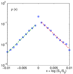
FIG. 1.: The relative frequency of intra-day returns (delay of 4 hours) for U.S. bonds over a period of 600 consecutive trading days beginning in March, 1985. For returns shown, it is approximately an asymmetric exponential distribution.

Analyses of financial markets have provided evidence for the assertion that successive variations of the return are uncorrelated [11, 14]. It implies that the distribution function $W(x,t)$ for returns $x(t)$ satisfies a Fokker-Planck equation [15, 6]

$$\frac{\partial W}{\partial t}=-B\frac{\partial W}{\partial x}+\frac{1}{2}\frac{\partial^{2}}{\partial x^{2}}(DW),$$ (5)

$D\equiv D(x,t)$ being the diffusion coefficient. The drift rate $B$ is assumed to be constant for intra-day fluctuations [16]. Following conclusions from studies of financial markets [7, 11], we limit our considerations to solutions that have a scaling form,

$$W(x,t)=\frac{1}{t^{\eta}}F(u).$$ (6)

Here $u=x/t^{\eta}$, and $\eta$ is referred to as the “drift exponent.” Notice that the pre-factor $t^{-\eta}$ is introduced in order that $W(x,t)$ is normalized for all $t$.

Consider first the case $B=0$. Financial markets exhibit the following behavior; a stock whose price $S(t)$ deviates significantly (up or down) from $S_{0}$ is traded at a higher frequency; i.e., the local diffusion rate $D(x,t)$ is enhanced. This effect is further amplified if the variation occurs during a shorter time interval. These observations are quantified in an assumption that $D(x,t)$ is a bi-linear function of $u$,

$$D(x,t)=\frac{1}{\gamma^{2}}(1-\gamma u)\bar{\Theta}(u)+\frac{1}{\nu^{2}}(1+\nu u)\Theta(u).$$ (7)

Here $\Theta(u)$ denotes the Heaviside $\Theta$-function and $\bar{\Theta}(u)=1-\Theta(u)$. As will become apparent momentarily, for $W(x,t)$ to be asymmetric, it is necessary for the parameters $\gamma$ and $\nu$ to be different. Notice that for larger values of $u$, nonlinear corrections to $D(x,t)$ may be required.

These assumption on the absence of correlations between successive movements of the return, and the scaling hypotheses (6) and (7) provide a unique value for $\eta$. This can be seen from Eqn. (5), which simplifies to

$$-\frac{\eta}{t^{\eta+1}}F(u)-\frac{\eta}{t^{\eta+1}}uF^{\prime}(u)=\frac{1}{2}\frac{1}{t^{3\eta}}(DF)^{\prime\prime}(u).$$ (8)

Consequently $\eta=1/2$, in agreement with conclusions from the analysis presented in Ref. [7] which show that the standard deviation of $W(x,t)$ for the S&P500 time series increases approximately as $\sigma(t)\sim t^{0.53}$.

Next, substituting the diffusion coefficient (7) in Eqn. (8) for $x>0$ gives,

$$\left(\frac{1+\nu u}{\nu^{2}}\right)F^{\prime\prime}(u)+\left(u+\frac{2}{\nu}\right)F^{\prime}(u)+F(u)=0.$$ (9)

Writing $F(u)=\sum_{n=0}a_{n}u^{\beta+n}$ [17], it is found that $F(u)\sim exp(-\nu u)$ is one of the solutions [18]. Combining it with the corresponding analysis for $x<0$ provides the solution

$$W(x,t)=\frac{A}{\sqrt{t}}e^{\gamma u}\bar{\Theta}(u)+\frac{B}{\sqrt{t}}e^{-\nu u}\Theta(u)$$ (10)

to the Fokker-Planck equation. Two conditions are required to evaluate the coefficients $A$ and $B$. Normalizing $W(x,t)$ gives

$$\frac{A}{\gamma}+\frac{B}{\nu}=1.$$ (11)

The second condition imposed is the continuity of the probability current $j(x,t)=-(DW)_{x}$, without which probability would accumulate at the origin. Using $\Theta^{2}(u)=\Theta(u)$, $\Theta_{u}(u)=\delta(u)$, $\bar{\Theta}_{u}(u)=-\delta(u)$ and $f(u)\delta(u)=f(0)\delta(u)$,

$$j(x,t)= - \frac{\gamma^{2}ue^{\gamma u}}{(\gamma+\nu)t}\bar{\Theta}(u)-\frac{\nu^{2}ue^{-\nu u}}{(\gamma+\nu)t}\Theta(u)$$ (12)

$$+ \frac{1}{t}\left(\frac{B}{\nu^{2}}-\frac{A}{\gamma^{2}}\right)\delta(u).$$ (13)

Hence, continuity of $j(x,t)$ at $u=0$ implies that

$$\frac{A}{\gamma^{2}}=\frac{B}{\nu^{2}}.$$ (14)

Thus $A=\gamma^{2}/(\gamma+\nu)$ and $B=\nu^{2}/(\gamma+\nu)$. Notice that $W(x,t)$ contains a discontinuity at the origin of $(\gamma-\nu)/\sqrt{t}$. Notice also that the mean value $\left<x(t)\right>=0$ for all $t$ and that the variance is $2t/\gamma\nu$; in particular, $W(x,t=0)=\delta(x)$, as required by the initial condition.

We make two further observations. If $D(x,t)$ is translated by $\Delta$, then the corresponding solution to the Fokker-Planck equation is $W(x-\Delta,t)$; however, the requirement $\left<x(t=0)\right>=0$ forces $\Delta=0$. Second, the solution for the general case (i.e., $B\neq 0$) is obtained by Galilean transformations of $D(x,t)$ and $W(x,t)$. This can be achieved by replacing $u$ by $(x-Bt)/\sqrt{t}$. For this case $\left<x(t)\right>=Bt$.

These conclusions were tested by investigating the following two types of random walks (for the case $B=0$). In the first, fixed-step-size walk (i.e., each step has a unit magnitude), the time interval for a step from a location $x(t)$ is chosen to be $\gamma^{2}/(1-\gamma u)$ if $u<0$ and to be $\nu^{2}/(1+\nu u)$ if $u\geq 0$. In the second, fixed-step-time walk (i.e., each step takes a unit time) the size of a step is chosen to be $\sqrt{(1-\gamma u)}/\gamma$ or $\sqrt{(1+\nu u)}/\nu$ depending on whether $u<0$ or $u\geq 0$. In each case the motion begins at the origin, and the direction of each step is chosen randomly with equal probability. The effective diffusion coefficient for these random walks is given by Eqn. (7) [6].

Figure 2(a) shows the histogram of positions for 5 million fixed-step-time walks of 256 steps, which is clearly consistent with $W(x,t)$ given by Eqn. (10). The mean value of the power spectra for these random walks, shown in Figure 2(b), exhibits a $k^{-2}$ decay; a similar behavior has been reported in an analysis of financial markets [7, 19].

One final point needs to be clarified prior to deriving formulae for valuation of options. Condition (1) implies that

$$G\equiv\frac{\gamma\nu-(\gamma-\nu)\sqrt{t}}{(\gamma+\sqrt{t})(\nu-\sqrt{t})}=e^{(b-B)t}.$$ (15)

Since this is not an identity, the equality cannot be valid for all $t$; hence a growth rate given by (1) is not consistent with the new theory. We propose to replace it by

$$\left<x(t)\right>=\left<\log\frac{S(t)}{S_{0}}\right>=bt.$$ (16)

This last condition imposed on our theory implies that the parameter $B$ in the Fokker-Planck equation is $b$.

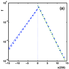
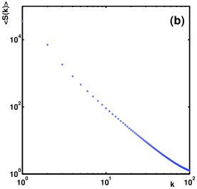
FIG. 2.: (a) The relative frequency of final locations for 5 million fixed-step-time walks of 256 steps. In this example $\gamma=10.0$ and $\nu=15.0$. The dashed lines show the distribution (10). (b) The mean $\left<S(k)\right>$ of the power spectrum for these random walks exhibits a $k^{-2}$ decay, similar to that observed in analyses of financial markets.

Now we are in a position to re-derive the formulae for pricing of options. Consider first, a European call to be exercised at time $t$. Pricing the option by its expected profit, it is found that

$$Ce^{rt} = e^{bt}G-K+K\zeta\frac{\gamma}{\gamma+\sqrt{t}}z^{\gamma/\sqrt{t}},\ \ \ z<1$$ (17)

$$= K\zeta\frac{\nu}{\nu-\sqrt{t}}z^{-\nu/\sqrt{t}},\ \ \ \ \ \ \ \ \ \ \ \ \ \ \ \ \ z\geq 1$$ (18)

where $z=(K/S_{0})exp(-bt)$ and $\zeta=\sqrt{t}/(\gamma+\nu)$.

A European put can be valued using the definition $P(S_{0},K,t)=e^{-rt}\int_{0}^{K}dS(K-S)f(S,t)$. When the return is distributed according to Eqn. (10),

$$Pe^{rt} = K-e^{bt}G+K\zeta\frac{\nu}{\nu-\sqrt{t}}z^{-\nu/\sqrt{t}},\ z>1$$ (19)

$$= K\zeta\frac{\gamma}{\gamma+\sqrt{t}}z^{\gamma/\sqrt{t}}.\ \ \ \ \ \ \ \ \ \ \ \ \ \ \ \ \ \ \ z\leq 1$$ (20)

Eqns. (18) and (20) can be used to justify the use of volatility smile curves to correct Black-Scholes pricing formulae. Suppose the “true” distribution of stock returns is (10), which decays slower than a Gaussian. Larger deviations of $x(t)$ will occur more frequently than predicted by the Gaussian distribution under this scenario (and will be noted by an observant trader). As a result, these options will be valued higher than the pricing given by the Black-Scholes theory. For a given strike price, this enhancement can be accounted for by increasing the “effective” volatility (used in the Black-Scholes formulae). As an example, consider a distribution $W(x,t)$ with $\gamma=15.0$ and $\nu=10.0$. (The annualized volatility for this distribution is 11.5%.) The “correct” valuation for options is assumed to be given by Eqns. (18) and  (20). We assign an effective volatility $V_{eff}$ at a strike price $K$ by equating the sum of prices of a call and a put estimated from the Black-Scholes theory (i.e., Eqns. (2) and (4)) with the corresponding sum for the new theory; i.e., $V_{eff}(K)$ is chosen so that

$$P_{BS}(S_{0},K,t)+C_{BS}(S_{0},K,t)=P(S_{0},K,t)+B(S_{0},K,t).$$ (21)

The function $V_{eff}(K)$ (for $S_{0}=100$, $t=0.5$ years, $b=10\%$, and $r$ arbitrary), shown in Figure 3, resembles volatility smile curves used in financial trading.

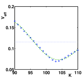
FIG. 3.: The effective volatility evaluated using Eqn. (21) for several values of the strike price $K$, in the neighborhood of the underlying stock price of 100 units. $\gamma$ and $\nu$ are 10.0 and 15.0 respectively, and the time to expiration of the option is half a year. The dashed line shows a quartic fit to the data, and the dotted line the standard deviation for the distribution.

We conclude by elaborating on a couple of issues raised by our work. The consensus value of a stock depends on many factors such as its historical performance and the market’s expectations for its future prospects. In the Black-Scholes theory, it is used to define the returns. Typically, $S_{0}$ is chosen to be the price of the stock at $t=0$. If a different value is used for $S_{0}$ (with a suitable modification of Eqn. (1)), the only effect is a uniform shift of $W(x,t)$; the pricing formulae remain unchanged. (Another way to state this is that the Langevin equation [6] is independent of $S_{0}$.) In contrast, $S_{0}$ plays a unique role in our theory. It is the value of the stock at which the diffusion coefficient reaches a minimum. Any deviation of the stock price from this value is reflected in an increase in the magnitude of its fluctuations. (The Langevin equation depends on $S_{0}$ through the diffusion coefficient $D(x,t)$.)

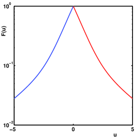
FIG. 4.: A solution $F(u)$ of the Fokker-Planck equation with a diffusion coefficient that includes a quadratic term in $u$. For this example, $\gamma=\nu=1.0$, and $\epsilon=-0.2$.

The second issue concerns possible higher order corrections to the bilinear form (7) for the diffusion coefficient. For example, if a quadratic term $\gamma^{-2}\epsilon u^{2}$ is added to $D(x,t)$ for $x>0$. Then, the ordinary differential equation satisfied by $F(u)$ changes to

$$(1+\nu u+\epsilon u^{2})F^{\prime\prime}(u) + (2\nu+4\epsilon u+\nu^{2}u)F^{\prime}(u)$$ (22)

$$+ (2\epsilon+\nu^{2})F(u)=0.$$ (23)

The solution for the symmetric case ($\gamma=\nu$) to this equation that satisfies the initial condition $F^{\prime}(0+)=-\nu F(0)$ is shown in Figure 4. $F(u)$ can be shown to decay as a power law for large $u$. Observations of such “fat-tails” have been made on distributions of inter-day returns [11, 7]. In spite of such possible corrections to the distribution $W(x,t)$, we believe that the theory presented here is still relevant in determining valuation of options. This is because, current frequency of trades (and not long time behavior of markets) is the information immediately available to traders, and on which their decisions are based. Hence, one may expect that distributions of intra-day variations in the return will determine the valuation of options.

The authors would like to thank K. E. Bassler, M. Dacorogna, G. F. Reiter and H. Thomas for discussions and their suggestions. GHG would also like to thank his colleges at TradeLink Corporation during 1989-1990. This research is partially funded by the National Science Foundation and the Office of Naval Research (GHG).

REFERENCES

- [1] N. Dunbar, “Inventing Money,” John Wiley & Sons, Ltd., Chischester, 2000.
- [2] F. Black and M. Scholes, J. Political Economy, 81, 637 (1973).
- [3] J. S. Cox and M. Rubinstein, “Option Markets,” Prentice-Hall (1985).
- [4] M. F. M. Osborne, in “The Random Character of Stock Market Prices,” Ed. P. Cootner, MIT Press, Cambridge, 1964.
- [5] This is the price assigned by the market on the basis of factors such as the historical performance and future expectations for the growth of a stock.
- [6] S. Chandrasekar, Rev. Mod. Phys., 15, 1 (1943).
- [7] R. N. Mantegna and H. E. Stanley, Nature, 376, 46 (1995); Nature, 383, 587 (1996).
- [8] S. Ghashghaie, W. Breymann, J. Peinke, P. Talkner, and Y. Dodge, Nature, 381, 767 (1996).
- [9] R. Friedrich, J. Peinke, and Ch. Renner, Phys. Rev. Lett., 84, 5224 (2000).
- [10] A. Arneodo, J.-F. Muzy, and D. Sornette, cond-mat/9708012 at lanl.arXiv.org.
- [11] M. M. Dacorogna, R. Gencay, U. Müller, R. B. Olsen, and O. V. Pictet, “An Introduction to High-Frequency Finance,” Academic Press, San Diego, 2001.
- [12] G. Bellocchi, M. M. Dacorogna, C. M. Hopman, U. A. Müller, and R. B. Olsen, J. Emp. Finance, 6, 479 (1999).
- [13] J. L. McCauley and G. H. Gunaratne, cs.CE/0201026 at lanl.arXiv.org.
- [14] A. Arneodo, J.-P. Bouchaud, R. Cont, J.-F. Muzy, M. Potters, and D. Sornette, cond-mat/9607120 at lanl.arXiv.org.
- [15] A. D. Fokker, Ann. d. Physik, 43, 812 (1914); M. Planck, Sitz. der preuss. Akad., p. 324 (1917).
- [16] Fokker-Planck equations with constant values for and have been used to describe dynamics of financial markets, see for example S. Maslov and Y.-C. Zhang, Physica A, 262, 232 (1999). Cascades in Financial markets (but not their dynamics) have been described using a Fokker-Planck equation with and dependent functions for and , see Ref. [9].
- [17] C. M. Bender and S. A. Orszag, “Advanced Mathematical Methods for Scientists and Engineers,” McGraw-Hill Book Company, New York, 1978.
- [18] The pre-factors in diffusion coefficient (7) was chosen in order to get an exponential solution for . The second solution to Eqn. (9) is given by where .
- [19] This form is observed for small values of . Generally, the spectrum is proportional to .