[

One-Dimensional Confinement and Enhanced
Jahn-Teller Instability in LaVO₃

Abstract

Ordering and quantum fluctuations of orbital degrees of freedom are studied theoretically for LaVO₃ in spin-C-type antiferromagnetic state. The effective Hamiltonian for the orbital pseudospin shows strong one-dimensional anisotropy due to the negative interference among various exchange processes. This significantly enhances the instability toward lattice distortions for the realistic estimate of the Jahn-Teller coupling by first-principle LDA+$U$ calculations, instead of favoring the orbital singlet formation. This explains well the experimental results on the anisotropic optical spectra as well as the proximity of the two transition temperatures for spin and orbital orderings.

]

Orbital degrees of freedom are playing key roles in magnetic and charge transport properties of transition metal oxides [2]. Especially it has been recognized that, in these strongly-correlated systems, spatial shapes of orbitals can give rise to an anisotropic electronic state even in the three-dimensional (3D) perovskite structure [3, 4]. There the spin ordering (SO) and orbital ordering (OO) are determined self-consistently [5].

Perovskite vanadium oxides, AVO₃ (A is rare-earth element), are typical $t_{2g}$ electron systems which show this interplay between orbital and spin degrees of freedom [6, 7, 8, 9, 10, 11]. Both magnetic and orbital transition temperatures, $T_{\rm N}$ and $T_{\rm o}$, respectively, change systematically according to the ionic radius of the A atom [12], which controls the bandwidth through the tilting of VO₆ octahedra. For smaller ionic radii (smaller bandwidth) such as A=Y, $T_{\rm o}$ for OO of G-type (3D staggered) is much higher than $T_{\rm N}$ for SO of C-type (rod-type) [11, 12]. As the ionic radius increases (the bandwidth increases), $T_{\rm o}$ decreases while $T_{\rm N}$ increases, and finally they cross between A=Pr and Ce [12]. In LaVO₃, the SO occurs at $T_{\rm N}\simeq 143$K first, and at a few degrees below $T_{\rm N}$ the OO takes place [13]. A remarkable aspect here is its proximity of $T_{\rm N}$ and $T_{\rm o}$, which is also observed for all the compounds with $T_{\rm N}>T_{\rm o}$, i.e., CeVO₃ [12] and La_1-xSr_xVO₃ ($x<0.17$) [13]. Therefore, in LaVO₃, the magnetic correlation appears to develop primarily and to induce the orbital transition immediately once the SO sets in.

Another interesting aspect of LaVO₃ is the large anisotropy in the electronic state, which has recently been explored by the optical spectra [14]. Figure 1 shows the temperature dependence of the spectral weights, $I_{c}$ along the $c$ direction and $I_{ab}$ within the $ab$ plane, which is obtained from the data in ref. REFERENCES. Here we define the spectral weight as an integration of the optical conductivity up to the isosbestic (equal-absorption) point at $2.8$eV, namely, $I_{\mu}\equiv\frac{2m_{0}}{\pi e^{2}n}\int_{0}^{2.8{\rm eV}}\sigma_{\mu}(\omega)d\omega$ ($\mu=c$ or $ab$), where $m_{0}$ and $n$ are the free electron mass and the density of V atoms, respectively. The most striking feature is the temperature dependence. $I_{c}$ grows rapidly below $T_{\rm N}$ while $I_{ab}$ is almost temperature independent. Therefore the temperature dependence is almost 1D although the ratio $I_{c}/I_{ab}\sim 2$ is not so large.

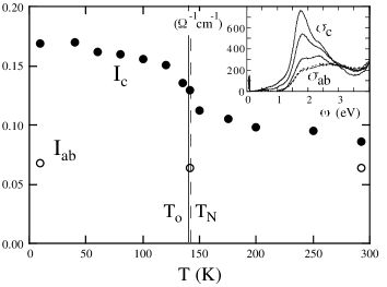
FIG. 1.: Temperature dependence of the spectral weight in LaVO₃. Filled and open circles represent the data along the $c$ axis $I_{c}$ and within the $ab$ plane $I_{ab}$, respectively. The inset shows the optical conductivity. The solid curves denote the data along the $c$ axis for $T=10,142,293$K from top to bottom, respectively. The data within the $ab$ plane are almost temperature independent which are shown by the dashed curves.

Compared with $e_{g}$ systems, the Jahn-Teller (JT) coupling in $t_{2g}$ systems is expected to be weak, and the quantum fluctuation and/or the singlet formation of the orbital degrees of freedom is a keen issue. Recently, Khaliullin et al. claimed that orbital singlet correlation along the $c$ axis is the driving force to realize the ferromagnetic spin exchange in the C-type antiferromagnetic (AF) phase in LaVO₃ [15]. On the other hand, the C-type SO state with the G-type OO has been obtained by the mean-field theory [16] and the first-principle calculation [17] which are justified for rather weakly-correlated cases and do not take account of quantum fluctuations seriously. There, the AF interactions within the $ab$ plane concomitant with a single occupation of $xy$ orbitals play a key role to stabilize the SO and OO. Hence, these two pictures are quite different. Since there are competing interactions with the orbital quantum nature, such as JT coupling and 3D orbital exchange couplings, it is highly nontrivial to what extent the quantum fluctuations are important under the realistic situations, nevertheless the quantitative study on this issue has been missing.

In this Letter, we study ordering and fluctuations of orbital degrees of freedom in the C-type AF phase in LaVO₃. An effective orbital model including the JT and the relativistic spin-orbit couplings is derived using the parameters obtained by first-principle LDA+$U$ calculations and the optical experiments. We show that the model exhibits a strong 1D anisotropy which explains well the experimental results for the optical spectra and the proximity of $T_{\rm o}$ to $T_{\rm N}$. It is concluded that the enhanced JT instability due to the 1D confinement dominates the orbital singlet formation in LaVO₃.

Now we derive the effective orbital model. We start from the strong-coupling limit of the Hubbard model with three-fold orbital degeneracy for the $t_{2g}$ orbitals [3]. The system contains two $d$ electrons at each V atom which form the high-spin $S=1$ state due to the Hund’s-rule coupling. To focus on the orbital sector in this spin-orbital coupled Hamiltonian, we assume the C-type SO. This is a reasonable approximation because the spin $S=1$ has less quantum nature compared to $S=1/2$ and the C-type SO is obtained by the mean-field calculation [16] and the first-principle calculation [17] as mentioned above. At the same time, we assume that the $xy$ orbital is singly occupied at each V atom, which drives the AF coupling in the $ab$ plane [16, 17]. Then the second electron goes to either $yz$ or $zx$ orbital. We assign a pseudospin state $\tau^{z}=\pm 1/2$ for the occupancy of these two orbitals [15]. Finally, our total Hamiltonian is written as ${\cal H}={\cal H}_{\rm orb}^{c}+{\cal H}_{\rm orb}^{ab}+{\cal H}_{\rm JT}+{\cal H}_{LS},$ each term of which is described below.

The orbital exchange term for the $c$ direction is

$${\cal H}_{\rm orb}^{c}=\sum_{\langle ij\rangle}J_{c}({\vec{\tau}}_{i}\cdot{\vec{\tau}}_{j}-1/4),$$ (1)

while that within the $ab$ plane is

$${\cal H}_{\rm orb}^{ab}=\sum_{\langle ij\rangle}\big{(}J_{ab}^{-}\tau_{i}^{z}\tau_{j}^{z}-J_{ab}^{+}/4-J_{ab}^{xy}/4\big{)}.$$ (2)

Here the summations are taken for nearest-neighbor pairs. The coupling constants are given by

$$J_{c} = 4t^{2}/(U^{\prime}-J_{\rm H}),$$ (3)

$$J_{ab}^{\pm} = \frac{2t^{2}}{3(U^{\prime}-J_{\rm H})}+\frac{4t^{2}}{3(U^{\prime}+2J_{\rm H})}\pm\frac{t^{2}}{U+2J_{\rm H}}\pm\frac{t^{2}}{U},$$ (4)

$$J_{ab}^{xy} = 4t^{2}/(U+2J_{\rm H})+4t^{2}/U,$$ (5)

where $U,U^{\prime}$ and $J_{\rm H}$ are the intra-orbital, the inter-orbital Coulomb interaction and the Hund’s-rule coupling, respectively. Neglecting the small tilting of VO₆ octahedra in LaVO₃, the transfer integral $t$ is taken to be diagonal which strongly depends on the direction, for instance, $t_{ij}^{yz}=t_{ij}^{zx}=t$ and otherwise zero in the $c$ direction. From the analysis in ref. REFERENCES, the parameters are estimated as $U\simeq 2.25$eV, $U^{\prime}\simeq 1.93$eV and $J_{\rm H}\simeq 0.16$eV. The transfer integral $t$ is set to be $0.12$eV based on the estimate of the bandwidth $\simeq 1$eV in first-principle calculations [17]. Then the orbital exchange interaction along the $c$ axis is estimated as $J_{c}\simeq 33$meV, while $J_{ab}^{-}\simeq 2$meV. We set $J_{c}=1$ as an energy unit in the following calculations.

Here we point out two important features in eqs. (1) and (2). One is that the exchange in the $c$ direction is Heisenberg-type while that within the $ab$ plane is Ising-type. From this, one might expect a strong quantum fluctuation in the $c$ direction as pointed out in ref. REFERENCES. However, this quantum nature becomes relevant only when the JT coupling is negligibly small, and this is not the case in LaVO₃ as discussed in the following. The other important feature is the large 1D anisotropy in the orbital exchange couplings. Note that the negative interference among different perturbation processes occurs in the in-plane coupling $J_{ab}^{-}$ in eq. (4), which results in the ratio of the exchange couplings $J_{c}/J_{ab}^{-}\sim 17$.

The JT coupling in the subspace of $\tau$ is given by

$${\cal H}_{\rm JT}=\sum_{i}gQ_{i}\tau_{i}^{z}+\frac{1}{2}\sum_{i}Q_{i}^{2},$$ (6)

where $Q_{i}$ is the JT phonon coordinate at site $i$. We neglect the kinetic energy of phonons, namely, regard $Q_{i}$ as a classical variable. It is crucial to estimate the coupling constant $g$, and we have done the following first-principle calculation [18]. Assuming the tetragonal symmetry, we calculate the total energy as a function of the JT distortion as shown in Fig. 2. This gives the JT stabilization energy $\sim 27$meV, which approximately corresponds to $E_{\rm JT}\equiv g^{2}/8$ in our model. Thus we obtain the estimate $E_{\rm JT}\simeq 0.8J_{c}$ ($g\simeq 2.6$), which is appreciable and cannot be neglected as in ref. REFERENCES.

The last term is the relativistic spin-orbit coupling, which may be important in the $t_{2g}$ systems. We obtain the effective Hamiltonian by projecting the original form ${\cal H}_{LS}=\sum_{i}\lambda{\vec{L}}_{i}\cdot{\vec{S}}_{i}$ to the subspace of $\tau$ by using the experimental fact that the spins lie within the $ab$ plane [19]. Here ${\vec{L}}_{i}$ is the orbital angular momentum. Since $L_{x}$ has matrix elements between $xy$ and $(yz,zx)$ in this case, the spin-orbit interaction is represented by ${\cal H}_{LS}=\sum_{i}\zeta\tau^{z}_{i},$ where $\zeta\equiv\lambda^{2}/\Delta$ and $\Delta$ is the energy separation between $xy$ and ($yz,zx$) orbital levels. This indicates that the spin-orbit coupling corresponds to the pseudo magnetic field along the $z$ direction. Using $\lambda\sim 20$meV in V atom and the estimate of $\Delta\sim 1$eV in the band calculation [17], we estimate $\zeta\sim 0.4$meV$\sim 0.01J_{c}$. This is small enough to be neglected in the following calculations.

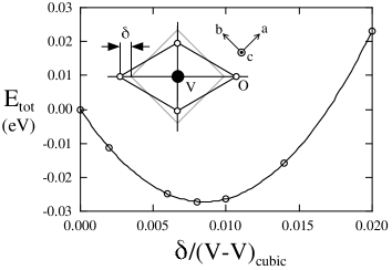
FIG. 2.: Total energy per V atom as a function of the Jahn-Teller distortion obtained by the LDA+$U$ calculation. The inset shows the tetragonal distortion of VO₆ octahedra considered here. The curve is a fit by a quadratic polynomial.

First we discuss the anisotropic temperature dependence in the spectral weight. The spectral weight is generally given by the kinetic energy of the system in the ground state $K$ as $I=-\pi K/4N$ where $N$ is the system size and we set $e^{2}=1$ [20]. In the strong-coupling limit, this is calculated by the exchange energy as shown below. Let us consider the Heisenberg model for the strong-coupling limit of the Hubbard model at half filling. The kinetic energy in the Hubbard model is calculated as $K=t\partial\langle{\cal H}\rangle/\partial t=\partial\langle{\cal H}\rangle/\partial\ln t$. Here the bracket denotes the expectation value in the ground state. Since the exchange coupling $J$ in the Heisenberg model is proportional to $t^{2}$, we obtain $I=-(\pi/4N)\times 2\partial\langle{\cal H}\rangle/\partial\ln J=-\pi\langle{\cal H}_{\rm Heis}\rangle/2N$ where ${\cal H}_{\rm Heis}$ is the Heisenberg Hamiltonian. Using this formula, we calculate the spectral weight for the present model by the exact-diagonalization in the ground state for $4\times 4$-site lattice embedded in the $ac$ plane. In Fig. 3 (a), the obtained values of $\Delta I_{c}\equiv-\pi J_{c}\sum\langle\vec{\tau}_{i}\cdot\vec{\tau}_{j}\rangle/2N$ and $\Delta I_{ab}\equiv-\pi J_{ab}^{-}\sum\langle\tau_{i}^{z}\tau_{j}^{z}\rangle/2N$ are plotted as a function of the JT coupling $g$. Note that these exchange correlations correspond to the enhancements of the spectral weights from the high-temperature limit to the ground state. The results indicate that, the contribution in the $c$ axis is much larger than that in the $ab$ plane. The ratio becomes larger than $20$ for the realistic value of $g\simeq 2.6$. This explains well the anisotropic temperature dependence of the spectral weight in Fig. 1.

We also discuss the magnitude of the total spectral weight in the ground state. Figure 3 (b) shows the calculated spectral weights $I_{\mu}=-\pi\langle{\cal H}_{\rm orb}^{\mu}\rangle/2N$ which include the contributions from the constants in eqs. (1) and (2). As shown in Fig. 3 (b), the ratio $I_{c}/I_{ab}$ is almost $1$ for the realistic value of $g$, which is much smaller than that of the temperature dependent part in Fig. 3 (a). This ratio is comparable but smaller than the experimental result $I_{c}/I_{ab}\sim 2$ in Fig. 1. This might be due to the facts that (i) the cut-off energy $2.8$eV for the integration is not large enough to take all the contribution of $I_{ab}$, and (ii) the transfer integrals for the different orbitals are different because they depend on the energy difference $\Delta_{dp}$ between the $d$ and the oxygen $p$ orbitals as the energy denominator. Since the huge anisotropy in temperature dependences is reproduced with the moderate anisotropy in the total weights, we believe that the orbital 1D confinement in our model plays a major role in the anisotropic electronic state in this material.

FIG. 3.: (a) Contributions depending on temperature and (b) total weights in the ground state for the spectral weight as a function of the Jahn-Teller coupling $g$.

We now turn to the discussion on the transition temperatures. In order to obtain the phase diagram at finite temperatures, we apply the transfer matrix method [21] combined with the unrestricted Hartree-Fock approximation for the interchain coupling $J^{-}_{ab}$ [22]. We start from a configuration of $\{Q_{i}\}$ and calculate the expectation value $\langle\tau_{i}^{z}\rangle$ numerically. Then, from the self-consistent equation $Q_{i}=-g\langle\tau_{i}^{z}\rangle$ which is obtained as the energy minimization for $Q_{i}$, we define a new configuration of $\{Q_{i}\}$. We repeat this procedure until $\{Q_{i}\}$ is optimized and the energy is minimized. In this treatment, $J^{-}_{ab}$ is effectively absorbed into the JT coupling $g$ as $\sum_{i}(gQ_{i}-2J_{ab}^{-}\langle\tau_{i}^{z}\rangle)\tau_{i}^{z}=-\sum_{i}\bar{g}^{2}\langle\tau_{i}^{z}\rangle\tau_{i}^{z}$ where $\bar{g}^{2}\equiv g^{2}+2J_{ab}^{-}$. The obtained transition temperature for the orbital/lattice ordering transition is plotted as a function of $\bar{g}$ in Fig. 4. We note that for large $g$, the transition temperature diverges as $T_{\rm o}\sim g^{2}/4$ which corresponds to the JT energy gap. However, this is an artifact of the mean-field-type treatment, and in reality $T_{\rm o}$ should stay at a constant of the order of $J_{c}$ since the coupling by $J_{c}$ between the neighboring sites determines $T_{\rm o}$ in the limit of large $g$.

Considering the realistic value of $J_{c}\simeq 33$meV and $E_{\rm JT}\simeq 27$meV ($g\simeq\bar{g}\simeq 2.6$) for LaVO₃, the orbital transition temperature is estimated as $T_{\rm o}\sim 800$K which is much higher than the observed $T_{\rm N}\simeq 143$K as indicated in Fig. 4. One might think that this contradicts with the experimental fact $T_{\rm N}>T_{\rm o}^{\rm exp}$. However the phase diagram is obtained assuming the C-type SO, which induces the 1D confinement of the orbital degrees of freedom with the enhanced $J_{c}$. Note that the disorder of the spins should reduce the effective orbital exchange as easily shown in the spin-orbital coupled Hamiltonian. It is also well-known that 1D systems have an enhanced instability to lattice distortions compared with higher dimensions. Therefore, $T_{\rm o}^{\rm 1D}=T_{\rm o}$ under this 1D orbital confinement can be higher than $T_{\rm o}^{\rm 3D}$ without the SO when the JT coupling governs the OO transitions. In real materials with $T_{\rm o}>T_{\rm N}$, $T_{\rm o}^{\rm 3D}$ decreases as the bandwidth increases, which indicates the relevance of the JT coupling. (If the 3D orbital exchange couplings dominate, $T_{\rm o}^{\rm 3D}$ should increase as $T_{\rm N}$ does.) Then, when the inequality $T_{\rm o}^{\rm 3D}<T_{\rm N}<T_{\rm o}^{\rm 1D}$ is satisfied, the OO transition with the JT lattice distortion should take place as soon as the SO grows and induces the 1D confinement in the orbital channel. In this scenario, comparing $T_{\rm o}^{\rm 1D}$ with $T_{\rm N}$, we can estimate the lower bound for the value of $g$ to realize this proximity of the transition temperatures. Our estimation for this lower bound from Fig. 4 is $g\sim 1$ which is consistent with the estimate in Fig. 2.

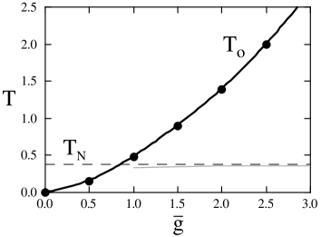
FIG. 4.: Transition temperature of the orbital ordering under the 1D confinement by the C-type AF spin order. For comparison, the experimental value of $T_{\rm N}$ in LaVO₃ is shown by the dashed line. The gray curve shows the expected $T_{\rm o}^{\rm exp}$. See the text for details.

Let us discuss this proximity of $T_{\rm N}$ and $T_{\rm o}^{\rm exp}$ by the Ginzburg-Landau type argument. In this spin-orbital coupled system, we have the term in which the SO parameter $M$ and the OO one $O$ are coupled as $\{a(T)-bM^{2}\}O^{2}$. Here $a(T)$ is the coefficient for the second-order term for OO without SO which is given by $a(T)=a^{\prime}(T-T_{\rm o}^{\rm 3D})$. Our results indicate the relation $a(T)-bM_{\rm sat}^{2}=a^{\prime}(T-T_{\rm o}^{\rm 1D}),$ where $M_{\rm sat}$ is the saturated magnetic moment. $T_{\rm o}^{\rm exp}$ is given by solving the equation $a(T_{\rm o}^{\rm exp})-bM^{2}(T_{\rm o}^{\rm exp})=0$. Assuming $M(T)=M_{\rm sat}\sqrt{(T_{N}-T)/T_{N}}$ for simplicity, the difference between $T_{\rm N}$ and $T_{\rm o}^{\rm exp}$ is given by $\delta T/T_{\rm N}\equiv(T_{\rm N}-T_{\rm o}^{\rm exp})/T_{\rm N}=(T_{\rm N}-T_{\rm o}^{\rm 3D})/(T_{\rm N}+\Delta T),$ where $\Delta T=T_{\rm o}^{\rm 1D}-T_{\rm o}^{\rm 3D}$. Considering the systematic changes of $T_{\rm N}$ and $T_{\rm o}$ for A-site ions [12], we expect that $T_{\rm o}^{\rm 3D}$ is slightly lower than $T_{\rm N}$ in LaVO₃ and CeVO₃. Assuming $T_{\rm o}^{\rm 3D}=0.8T_{\rm N}$, we plot the expected $T_{\rm o}^{\rm exp}$ in Fig. 4 as the gray curve. For the realistic value of $g$, we have $T_{\rm o}^{\rm exp}$ quite close to $T_{\rm N}$ as observed in these compounds.

To summarize, we have investigated the role of orbitals to understand the electronic state in LaVO₃. We have derived the effective orbital model with strong one-dimensional anisotropy assuming the C-type spin ordering. We conclude that with the realistic Jahn-Teller coupling, the orbital 1D confinement leads to an enhanced instability toward lattice distortions suppressing the orbital quantum nature. This gives a comprehensive description of the anisotropy in the optical spectra and the proximity of the critical temperatures of magnetic and orbital transitions.

The authors appreciate Y. Tokura, S. Miyasaka, T. Arima, G. Khaliullin and B. Keimer for fruitful discussions. Part of numerical computations are done using TITPACK ver.2 developed by H. Nishimori, who is also thanked.

REFERENCES

- [1]
- [2] Y. Tokura and N. Nagaosa, Science 288, 462 (2000).
- [3] K. I. Kugel and D. I. Khomskĭ, Sov. Phys. Usp. 25, 231 (1982); K. I. Kugel and D. I. Khomskii, Sov. Phys. Solid State 17, 285 (1975).
- [4] M. Imada, A. Fujimori, and Y. Tokura, Rev. Mod. Phys. 70, 1039 (1998).
- [5] See for example R. Maezono, S. Ishihara, and N. Nagaosa, Phys. Rev. B 58, 11583 (1998).
- [6] A. V. Mahajan et al., Phys. Rev. B 46, 10966 (1992).
- [7] H. C. Nguyen and J. B. Goodenough, Phys. Rev. B 52, 324 (1995).
- [8] H. Kawano, H. Yoshizawa, and Y. Ueda, J. Phys. Soc. Jpn. 63, 2857 (1994).
- [9] Y. Ren et al., Phys. Rev. B 62, 6577 (2000).
- [10] M. Noguchi et al, Phys. Rev. B 62, 9271 (2000).
- [11] G. R. Blake et al., Phys. Rev. Lett. 87, 245501 (2001).
- [12] S. Miyasaka and Y. Tokura, private communications.
- [13] S. Miyasaka, T. Okuda, and Y. Tokura, Phys. Rev. Lett. 85, 5388 (2000).
- [14] S. Miyasaka, Y. Okimoto and Y. Tokura, J. Phys. Soc. Jpn. 71, 2086 (2002).
- [15] G. Khaliullin, P. Horsch, and A. M. Oleś, Phys. Rev. Lett. 86, 3879 (2001).
- [16] T. Mizokawa and A. Fujimori, Phys. Rev. B 54, 5368 (1996).
- [17] H. Sawada et al., Phys. Rev. B 53, 12742 (1996).
- [18] The calculation was done by using plane-wave pseudopotential method based on the LDA+ scheme [Z. Fang et al., J. Phys.: Cond. Matt. 14, 3001 (2002)] with eV to reproduce the band gap properly.
- [19] V. G. Zubkov et al., Sov. Phys. Solid State 15, 1079 (1973).
- [20] P. Maldague, Phys. Rev. 16, 2437 (1977).
- [21] M. Suzuki, Phys. Rev. B 31, 2957 (1985); H. Betsuyaku, Prog. Theor. Phys. 73, 319 (1985). In the numerical calculations, we apply extrapolations in both the Trotter number and the system size .
- [22] D. J. Scalapino, Y. Imry, and P. Pincus, Phys. Rev. B 11, 2042 (1975).