Trap Models and Slow Dynamics in Supercooled Liquids

Abstract

The predictions of a class of phenomenological trap models of supercooled liquids are tested via computer simulation of a model glass-forming liquid. It is found that a model with a Gaussian distribution of trap energies provides a good description of the landscape dynamics, even at temperatures above $T_{c}$, the critical temperature of mode-coupling theory. A scenario is discussed whereby deep traps are composed of collections of inherent structures above $T_{c}$ and single inherent structures below $T_{c}$. Deviations from the simple Gaussian trap picture are quantified and discussed.

Glass-forming systems are ubiquitous in nature, and constitute the basis for wide-ranging technological applications [1, 2]. Furthermore, the theoretical and computational techniques developed for the study of glass-forming liquids have been extremely useful in the study of static and dynamic phenomena in other complex systems, such as spin-glasses, polymers and proteins [3]. Unfortunately, despite recent progress, the underlying microscopic origin of slow dynamics in supercooled liquids remains largely an unsolved problem.

The mode-coupling theory (mct), pioneered by Götze and co-workers, is unique in that quantitative predictions are made for the viscous slowing-down exhibited by dynamical correlators with the input of structural information alone [4]. In this sense, mct is perhaps the only ab initio theory of slow dynamics in supercooled liquids. mct appears to be a quantitative theory of cage formation at intermediate times, but has some shortcomings in describing cage relaxation at long times. In particular, mct overestimates the the cage effect, leading to a “glass-transition” at a temperature $T_{c}>T_{g}$ where $T_{g}$ is the experimentally determined glass transition temperature. Theoretical attempts have been made to include “hopping” processes that restore ergodicity below $T_{c}$, however such theories currently demand a level of approximation that reduces the ability to make quantitative predictions [4].

A seemingly different perspective is provided by the “landscape” picture of slow dynamics in supercooled liquids [5, 6]. Here, one attributes slow structural relaxation to the complex pathways that connect configurational states or “inherent structures”(is) on the multidimensional potential surface. Wales and coworkers have performed extensive studies of the details of the landscape properties of model glass forming liquids [7, 8]. In particular, they have noted that the landscape of Lennard-Jones liquids has a multi-funnel structure. The inherent structures residing inside a funnel are separated by small barriers, while barriers separating funnels may be large. Heuer and coworkers [9, 10, 11] have recently shown that the phase point of an unbiased trajectory is trapped in a “meta-basin” for long periods of time, making frequent small hops within the meta-basin, and infrequent excursions from one meta-basin to another, a scenario that that resonates with the multi-funnel picture.

On the other hand, recent studies of mean field p-spin glasses [3] have established a deep connection between the mct and landscape pictures. The mct transition temperature $T_{c}$ appears as the point below which the only available saddle points of the energy are minima, whereas above $T_{c}$, the vast majority of saddles are higher order saddles [12]. Within mct (or mean field p-spin glasses), the dynamics freezes at $T_{c}$ in the lowest available ‘critical’ saddle that percolates in phase-space, but never penetrates the lower minima region below $T_{c}$. This is related to the above mentioned inability of mct to describe hopping events.

The relevance of this result for Lennard-Jones systems was discussed in the important work of Angelani et al. [13] and Broderix, Cavagna et al. [14, 15], where the critical mct temperature $T_{c}$, as identified from the extrapolated divergence of dynamical time scales, coincides with the point where the number of unstable saddles vanishes. However, due to the non mean-field nature of the system, several important differences with mct appear. First, because barriers are finite, the dynamics below $T_{c}$ is now dominated by activated transitions between basins of local minima (is), and not by the exploration of the “critical” saddle. As was shown in [16, 17], there indeed exists a separation of time scales between vibrational motion within an is, and hopping between is, as envisioned long ago by Goldstein [6]. Second, the vanishing of saddles below $T_{c}$ and the inexistence of minima above $T_{c}$ are no longer sharp statements. One of the primary goal of the present paper is to actually show that the long time dynamical properties are indeed governed by these rare, deep traps, even above $T_{c}$. The landscape studies of Wales et al. [7, 8] and Heuer et al. [9, 10, 11] suggest that an activated dynamics of a more complex variety, namely escape from a meta-basin may be taking place already above $T_{c}$. In this context, it is interesting to note that some theories of slow dynamics posit that activated processes are directly responsible for the onset of non-Arrhenius relaxation at temperatures far above $T_{c}$ [18].

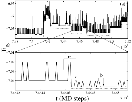
Figure 1: is (solid line) and meta-basins (dotted line) visited during the course of a 70 particle MD run at $T^{*}=0.49$. The dotted line is slightly shifted along the energy axis for better clarity. is transitions within a meta-basin are denoted $\beta$ while transitions from one meta-basin to another are denoted $\alpha$. The is energies are divided by the total number of particles in the system.

A simple way of rationalizing glassy dynamics in the regime where activation between attractors is the dominant mechanism is provided by the “trap” model advocated in [19]. In this picture, the dynamics of a coherent subregion of the system is summarized by the motion of a single point evolving in a landscape of “valleys” or “traps”, separated by barriers that can only be overcome via activation. The wandering of the phase point is described by a simple master equation with hopping rates that encode the statistics of barrier heights and the geometry of phase space. The simplest of the trap models assumes that the top of the landscape is flat, and thus the rate of escape from a trap is related only to the trap depth. If one further assumes that the probability to reach any new trap is identical, the specification of the distribution of trap energies determines the behavior of all dynamical observables. Interestingly, Ben Arous et al. [20] have shown that for a finite size p-spin model, the short time dynamics are identical to that predicted by mct, but the long time dynamics are precisely given by the trap model predictions. The purpose of this work is to make concrete connections between the landscape properties of a model glass forming liquid, and the trap picture above the glass temperature. The relevance of the trap picture to describe aging dynamics in the glass phase will be discussed in a later work.

The system that we study is the modified 80-20 Lennard-Jones system studied by Sastry et al. [16], and we refer the reader to this work for the details. Since the macroscopic liquid should be viewed as a partitioning of noninteracting ‘coherent’ cells within which the landscape picture is sensible [9, 10, 11, 21], we study small systems containing between 70 and 150 particles. Long (up to $2\times 10^{9}$ total time steps) series of inherent structures are produced from long molecular dynamics runs at various temperatures between $T^{*}$ = 0.85 and $T^{*}$ = 0.49 ($T_{c}\approx 0.45$). This corresponds to a total time run of up to 13 $\mu s$. Quenches are generated at intervals much shorter than the $\alpha$-relaxation time at a given temperature from a combined steepest descent and conjugate gradient algorithm. This procedure is sufficient to resolve nearly all significant inherent structure transitions.

In Fig.1 we show a portion of an is history verses time ($E_{IS}(t)$ vs $t$) for $T^{*}$ = 0.490. One notes several remarkable features in this time series [11]. First, long regions where the system switches between only a few elementary is exist. Such long-lived collections of is clearly provide deep trap states. Using the meta-basin definition of Büchner and Heuer [9], the time series of is may be mapped into a time series of the visited meta-basins. Transitions between is within a meta-basin involve very small flexing of a cage, while transitions between meta-basins (signifying release from a trap) involve collective rearrangements of particles. This observation is fully consistent with Stillinger’s landscape picture of the $\beta$ and $\alpha$ processes, whereby the $\beta$ process corresponds to transitions between is within the meta-basin, while the $\alpha$ process corresponds to transitions between meta-basins [5]. Visual inspection demonstrates clearly that deeper trap states are longer lived, in accordance with the trap model [19]. It is important to note that although the is energy is used a label of the instantaneous state of the system, no assumptions are made concerning the transition dynamics between meta-basins. In particular, nontrivial entropic factors may contribute to dynamics of meta-basin transitions.

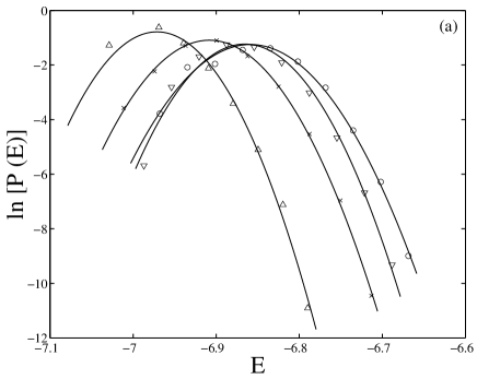
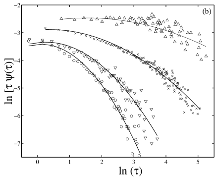
Figure 2: (a) Distribution of meta-basin energies (per particle) for $T^{*}$ = 0.490, 0.575, 0.669 and 0.764 (from left to right). The solid lines are the Gaussian fits for the corresponding temperature. (b) Distribution of hopping times from meta-basins in a 70 particle system for $T^{*}$ = 0.764, 0.669, 0.575, and 0.490 (from left to right). The curves are shifted in time to fit inside the figure.

In simple trap models, the fundamental quantity is the distribution of trap depths. The most commonly used model assumes an exponential distribution of trap energies, i.e. $\rho(E)=\left(1/T_{0}\right)\exp\left(-E/T_{0}\right)$. This model yields a power law distribution of trapping times $\psi(\tau)\sim\tau^{-(1+\frac{T}{T_{0}})}$, and a power law correlations for simple dynamical variables [19, 22, 23, 24, 25]. This model also has a strict glass transition at the temperature $T_{0}$. Other trap models, such as the Gaussian model with $\rho(E)=\left(\frac{\exp(-(E-\overline{E})^{2}/E_{0}^{2})}{\sqrt{\pi}E_{0}}\right)$ also display glassy phenomenology, such as a super-Arrhenius growth of the relaxation time, stretched exponential decay and (interrupted) aging [19].

Assuming that the meta-basins form traps, the computed distribution of trap energies may be calculated directly. At all temperatures studied, the distribution is well fitted by a Gaussian, as shown in Fig.2(a). Previous studies have demonstrated that the distribution of inherent structures (not meta-basins) is Gaussian [10, 26, 27].

Figure 3: Correlation function $C(t)$ as defined in the text. Both power law and stretched exponential fits are shown. The data clearly supports the stretched exponential fit over the power law fit. The solid line is for $T^{*}$ = 0.490 and dotted line is for $T^{*}$=0.575.

Given simple activated dynamics to leave a trap of depth $E$, i.e. trap lifetimes $\tau=\tau_{0}\exp(\beta E)$, the distribution of trapping times may be computed. For the Gaussian trap model, this yields a distribution of trapping times $\psi(\tau)=\frac{1}{\tau\sqrt{\pi}\Delta}\exp\left(-\left(\frac{\ln(\tau/\tau_{0})}{\Delta}\right)^{2}\right)$, where $\Delta\equiv\beta E_{0}$. Note that the product $\tau\psi(\tau)$ is log-normal. In Fig.2(b) we show fits of $\ln(\tau\psi(\tau))$ vs. $\ln(\tau)$. The log-normal behavior predicted by the Gaussian trap model fits remarkably well over a wide range of time scales. The attempt time $\tau_{0}$ is determined to be on the order of $\sim 1ps$, reasonable for the “vibrational” prefactor of an activated process in a dense Lennard-Jones liquid. Given that meta-basins can have lifetimes spanning up to a fraction of one $\mu s$, there clearly exists a separation of time scales between inter- and intra-trap (meta-basin) motion. This timescale separation does not exist at the level of single is above $T_{c}$. It is interesting to note that previous computational studies have determined power law waiting time distributions in a variety of systems [11, 28, 29]. On the basis of a plot of $\ln\psi(\tau)$ vs. $\ln(\tau)$ it is difficult to detect the distinction between the power law and log-normal versions of $\psi(\tau)$, while plots of $\ln(\tau\psi(\tau))$ vs. $\ln(\tau)$ clearly reveal this distinction. The Gaussian widths $\Delta$ determined from fits of $\psi(\tau)$ are larger than $\beta E_{0}$ determined from $\rho(E)$ directly. This fact shows that one of the crude assumptions of the trap model cannot be taken literally; for example the energy depth of the meta-basin alone does not determine the absolute barrier for trap escape. Interestingly, the nontrivial entropic and saddle point dependence of $E_{0}$ only quantitatively, and not qualitatively affects estimates of the distribution of trapping times.

We now compare simple dynamical predictions of the Gaussian trap model to computer simulations in the Lennard-Jones mixture. The basic quantity investigated is $C(t)=\langle\delta\epsilon_{T}(t)\delta\epsilon_{T}(0)\rangle$, namely, the correlation function of fluctuations of visited meta-basin depths. In the exponential trap model, $C(t)$ decays as a power law, while for the Gaussian model the behavior of $C(t)$ may be approximated with a stretched exponential decay [19]: $C(\tau)\sim\exp\left(-(a(T)t^{b(T)})\right)$, with a stretching coefficient $b(T)\sim\left(1+\frac{1}{2}(\Delta)^{2}\right)^{-\frac{1}{2}}$. For the range of temperatures studied, the Gaussian trap prediction of stretched exponential relaxation is reasonably well borne out, as is shown in Fig.3. Approximate stretched exponential dependence is seen for all temperatures $T^{*}\leq 1$. At the two lowest temperatures studied in this work ($T^{*}$ = 0.575 and $T^{*}$ = 0.490) where the extracted values of $b(T)$ are most accurate, the extracted values of $b(T)$ are $b(0.575)$ = 0.68$\pm$0.1 and $b(0.490)$ = 0.61$\pm$0.05, respectively. The values predicted from the trap model are $b(0.575)$ = 0.45$\pm$0.05 and $b(0.490)$ = 0.41$\pm$0.1, respectively. Thus, the predicted values are in reasonable agreement with the values extracted from simulation [30].

Our results show that activated process are important even above $T_{c}$ in supercooled liquids. This does does not contradict the applicability of mct to describe short time dynamics in this regime, nor does it contradict the results of [13, 14, 15], which show that most accessible saddles are unstable above $T_{c}$. The long time dynamics, however, will be dominated by rare, deep traps. Our work is consistent with this, provided that traps (meta-basins) smoothly transition from a collection of connected inherent structures above $T_{c}$ to single inherent structures below $T_{c}$. That is, above $T_{c}$ the barriers separating the inherent structures inside a meta-basin are small compared to temperature, while below $T_{c}$ they are large. Computer simulation evidence supports this picture [16]. This would imply that the simple “single-level” trap model above $T_{c}$ should become a “multi-level” trap picture below $T_{c}$ [3], where interesting aging effects should then take place as in spin-glasses [32].

We gratefully acknowledge useful discussions with E. Bertin, B. Chakraborty, D. Das, I. Giardina, C. Godrèche, A. Heuer, J. Klafter, J. Kondev, and R. Yamamoto. D.R.R. and R.A. Denny acknowledge the NSF for financial support.

References

- [1] See, for example, the special issue on glasses and glass forming liquids [Science 267 (1995)].
- [2] M.D. Ediger, C.A. Angell, and S.R. Nagel, J.Phys.Chem. 100 13200 (1996).
- [3] See reviews in Spin Glasses and Random Fields A.P. Young, Editor, World Scientific, Singapore (1998).
- [4] W. Götze, and L. Sjögren, Rep. Prog. Phys. 55, 241 (1992).
- [5] F.H. Stillinger, Science, 267, 1935, (1995).
- [6] M. Goldstein, J. Chem. Phys. 51, 3728 (1969).
- [7] D.J. Wales, J.P.K. Doye, M.A. Miller, P.N. Mortenson, and T.R. Walsh, Adv. Chem. Phys. 115, 1 (2000).
- [8] T.F. Middleton, and D.J. Wales, Phys. Rev. B, 64 024205, (2001).
- [9] S. Büchner, and A. Heuer, Phys. Rev. Lett., 84, 2168, (2000).
- [10] S. Büchner, and A. Heuer, Phys. Rev.E 60, 6507 (1999).
- [11] B. Doliwa, and A. Heuer Hopping in a Supercooled Lennard-Jones Liquid: Metabasins, Waiting Time Distribution, and Diffusion, cond-mat/0205283.
- [12] J. Kurchan and L. Laloux, J. Phys. A29, 1929, (1996).
- [13] L. Angelani, R. Di Leonardo, G. Ruocco, A. Scala, and F. Sciortino, Phys. Rev. Lett. 85, 5356 (2000).
- [14] K. Broderix, K.K. Bhattacharya, A. Cavagna, A. Zippelius, and I. Giardina, Phys. Rev. Lett. 85, 5360 (2000).
- [15] A. Cavagna, Europhys. Lett. 53 490 (2001).
- [16] S. Sastry, P.G. Debenedetti, and F.H. Stillinger, Nature (London), 393, 554, (1998).
- [17] T.B. Schroder, S. Sastry, J.C. Dyre, and S.C. Glotzer, J. Chem. Phys., 112, 9834 (2000).
- [18] G. Tarjus, D. Kivelson, and P. Viot, J. Phys.: Condens. Matter 12, 6497 (2000).
- [19] C. Monthus, and J.-P. Bouchaud, J. Phys. A 29 3847 (1996), and refs. therein.
- [20] G. Ben Arous, A. Bovier, and V. Gayrard, Phys. Rev. Lett. 88, 087201 (2002).
- [21] R. Zwanzig, J. Chem. Phys. 79, 4507 (1983).
- [22] T. Odagaki, and A. Yoshimori, J. Phys.: Condens. Matter 12 6509 (2000).
- [23] T. Odagaki, Phys. Rev. Lett., 75, 3701 (1995).
- [24] J.T. Bendler, and M.F. Shlesinger, J. Stat. Phys., 53, 531, (1988).
- [25] E.W. Montroll, and M.F. Shlesinger, J. Stat. Phys., 32, 209, (1983).
- [26] S. Sastry, Nature, 409, 164 (2001).
- [27] F. Sciortino, W. Kob, and P. Tartaglia, Phys. Rev. Lett., 83, 3214 (1999).
- [28] P. Allegrini, J.F. Douglas, and S.C. Glotzer, Phys. Rev. E, 60, 5714, (1999).
- [29] J. Habasaki, and Y. Hiwatari, Phys. Rev. E, 59, 6962, (1999).
- [30] While the simulated values of and those predicted based on the Gaussian trap model with extracted from are in reasonable agreement (within the error bars), there is systematic tendency for the trap prediction to underestimate the value of . For large values of our statistics for are poor, however there does seem to be a slight systematic deviation from log-normal behavior for the largest ’s (not shown in Fig. 2(b)). Including this curvature change results in slightly larger estimates of . Doliwa and Heuer (private discussion) have demonstrated that their data is consistent with a Gaussian trap model, but with saddle-point values that depend somewhat on the trap depth. This observation is sufficent to explain the small deviations mentioned above. See also the related discussion in [31].
- [31] X. Xia and P. G. Wolynes, Phys. Rev. Lett. 86, 5526, (2001).
- [32] B. Rinn, P. Maass, and J.-P. Bouchaud, Phys. Rev. B 64, 104417, (2001).