Effect of the on-site Coulomb repulsion on superconductivity
in the boson-fermion model

Abstract

We study the influence of the repulsive Coulomb interactions on thermodynamic properties of the boson fermion model with an anisotropic ($d$-wave, and extended $s$-wave) order parameter. Superconductivity is induced in this model from the anisotropic charge exchange interaction between the conduction band fermions (electrons or holes) and the immobile hard-core bosons (the localized electron pairs). The on-site Coulomb repulsion competes with this pairing interaction and hence is expected to have a detrimental influence on superconductivity. We analyze this effect in some detail considering the two opposite limits of: the weak and strong repulsion. A possible crossover between both these regimes is also discussed.

I Introduction

The boson fermion (BF) model describes a mixture of the narrow band fermions coupled to a system of the composite hard-core bosons. Initially, this type of an effective Hamiltonian has been invented for a system of itinerant electrons interacting with the local lattice deformations in the crossover regime, between adiabatic and antiadiabatic limits Ranninger-85 . Later, the same model has been independently considered by a number of authors Eliashberg-87 ; Friedberg-89 ; Ioffe-89 ; Ranninger-95 as a possible scenario for a mechanism of the high temperature superconductivity (HTSC). There are also attempts to apply a similar BF model to explain certain aspects of the Bose condensed atoms of the alkali metals Holland-01 .

This model reveals a rich physics both in its: normal phase and the broken symmetry superconducting/superfluid state. As shown in the mean field type studies Friedberg-89 ; Ranninger-95 there is a characteristic temperature $T_{c}$ bellow which fermions are driven to the superconducting phase and simultaneously bosons start to Bose-condense. This result has been confirmed (neglecting the hardcore nature of bosons) by means of the shielded potential approximation Kostyrko-96 and with a help of the renormalization group approach Domanski-01 . Moreover, when approaching the critical temperature from above, the pairing-wise correlations start to manifest themselves strongly. In particular, they may give rise to a formation of the pseudogap in the fermion spectrum. This effect, known experimentally from a variety of measurements (see e.g. review paper Timusk-99 ), provides a firm argument for application of this model to describe the HTSC materials.

Pseudogap formation and its variation with a lowering temperature has been carefully investigated for the BF model using: a) the selfconsistent perturbative treatment of the boson-fermion coupling perturbative ; Ren-98 , b) the perturbative treatment of the kinetic processes (a là Hubbard I for the fermion hopping) with respect to the exact solution of this model in its atomic limit Domanski-98 , c) the dynamical mean field theory (DMFT) equations which have been selfconsistently solved within the noncrossing approximation for the auxiliary impurity problem DMFT , d) and the renormalization group technique Domanski-01 .

Many experimental data, especially the angle resolved photoemission spectroscopy ARPES , seem to suggest the anisotropic $d$-wave type structure of both: the pseudogap and true superconducting gap. However, there are also known some measurements, for instance the $c$-axis Josephson tunneling Kouznetsov-97 and the photoemission spectroscopy on Bi₂Sr₂CaCu₂O_8+δ Ma-95 , which provide the strong arguments for a nonzero $s$-wave ingredient of the order parameter. In a most realistic situation one can expect that the order parameter of the HTSC cuprates acquires a mixed $s+d$ or $s+$ i$d$ symmetry. Possibility for an appearance of the mixed symmetry superconducting phase has been theoretically explored on quite the general grounds using a 2-dimensional electron system with the anisotropic potential $V=V_{s}+V_{d}$ of the arbitrary (from weak to strong) attraction strength Musaelian-96 . So far, most of the studies of superconductivity within the BF model have been performed for the isotropic pairing interaction. Some attempts to analyze the $d$-pairing superconductivity together with a microscopic justification for introducing the BF type Hamiltonian can be found in the paper by Geshkenbein et al Geshkenbeim-97 . Very recently, a more formal way has been explored by Micnas et al Micnas-01 .

In this paper we shall investigate various kinds of the superconducting phase induced by an anisotropic potential of the BF model in a presence of the Coulomb interactions between fermions. For simplicity we shall concentrate only on a case of the on-site repulsion $U>0$, where $U=(ii|\frac{e^{2}}{|{\bf r}|}|ii)$ in the Wannier representation. In general, one expects that the on-site repulsion (which prevents fermions from forming the local pairs) would compete with the correlations induced by the boson-fermion coupling (this interaction is a driving force for the pairing in the BF model and is responsible for inducing the pseudogap at temperatures $T^{*}>T>T_{c}$ and the true superconducting gap when $T\leq T_{c}$). We shall address the following question: what is an extent of a detrimental influence of $U$ on the pairing correlations ?

The abovementioned competition has been already studied in a normal phase of the BF model using the nonperturbative approach of the DMFT Romano-01 . In our paper we shall investigate the anisotropic superconducting phase. To make our study feasible we assume that the pairing interactions are relatively weak (a meaning of this assumption is explained in the next section) and we try to estimate the influence of the Coulomb repulsion varying its intensity from the weak to strong interaction limits.

II The model

Hamiltonian of the system under consideration consists of the two parts $H=H^{BF}+H^{Coul}$. First of them refers to the standard BF model Hamiltonian Ranninger-95

$$H^{BF} = \sum_{{\bf k},\sigma}\left(\varepsilon_{\bf k}-\mu\right)c_{{\bf k},\sigma}^{\dagger}c_{{\bf k},\sigma}+\left(\Delta_{B}-2\mu\right)\sum_{i}b_{i}^{\dagger}b_{i}$$ (1)

$$+ \frac{1}{\sqrt{N}}\sum_{{\bf k},{\bf q}}\left(v_{{\bf k},{\bf q}}b_{\bf q}^{\dagger}c_{-{\bf k}+{\bf q}/2,\downarrow}c_{{\bf k}+{\bf q}/2,\uparrow}+\mbox{h.c.}\right)$$

and the second part denotes the on-site interaction between fermions $H^{Coul}=U\sum_{i}n_{i\downarrow}n_{i\uparrow}$. We use here the standard notations for annihilation (creation) operators of fermion $c_{i,\sigma}$ ($c_{i,\sigma}^{\dagger}$) with spin $\sigma$ and for the hard-core boson $b_{i}$ ($b_{i}^{\dagger}$) at site $i$ of the 2 dimensional square lattice. The indices ${\bf k}$ and ${\bf q}$ in (1) denote the coordinates of the momentum space. We assume the tight binding dispersion for fermions $\varepsilon_{\bf k}=-2t\left(\cos{k_{x}}+\cos{k_{y}}\right)$, and set the bandwidth $D=8t$ as a unit ($D\equiv 1$).

It is important to remark now that we let the boson-fermion exchange potential $v_{{\bf k},{\bf q}}$ to be anisotropic. As explained in the ref. Geshkenbeim-97 the low energy physics of this model is prevailed by bosons of small momenta $|{\bf q}|\simeq 0$. Usually, the magnitudes of the superconducting gap in HTSC materials are of the order of several $meV$ (which is $\sim 10^{-3}$ of the bandwidth $D$). It is thus reasonable to assume that the pairing potential $v_{{\bf k},{\bf q}}$, which establishes the energy scale for $T_{c}$ and $\Delta_{sc}(T=0)$, is small as compared to $D$. In such a case the following mean field decoupling is justified

$$\sum_{\bf q}v_{{\bf k},{\bf q}}b_{\bf q}^{\dagger}c_{-{\bf k}+{\bf q}/2,\downarrow}c_{{\bf k}+{\bf q}/2,\uparrow}\simeq$$

$$v_{{\bf k},{\bf q}={\bf 0}}\left(\left<b_{{\bf q}=\bf{0}}\right>^{*}c_{-{\bf k},\downarrow}c_{{\bf k},\uparrow}+b_{{\bf q}={\bf{0}}}^{\dagger}\left<c_{-{\bf k},\downarrow}c_{{\bf k},\uparrow}\right>\right).$$ (2)

We further write down the anisotropic potential $v_{{\bf k},{\bf 0}}$ as a product Micnas-01

$$v_{{\bf k},{\bf 0}}\equiv g\;\phi_{\bf k},$$ (3)

where $g$ characterizes the interaction strength and $\phi_{\bf k}$ stands for the dimensionless factor which has to reflect the fourfold symmetry of CuO₂ planes of the HTSC cuprates. In general the anisotropy factor $\phi_{\bf k}$ can be represented as

$$\phi_{\bf k}=\alpha_{0}+\alpha_{s}\left(\cos{k_{x}}+\cos{k_{y}}\right)+\alpha_{d}\left(\cos{k_{x}}-\cos{k_{y}}\right)$$ (4)

and the coefficients $\alpha_{0,s,d}$ denote a relative contribution of the isotropic, the extended $s$-wave, and the $d$-wave part into the order parameter of the superconducting phase. They should be adjusted depending on a specific material. If for example $\alpha_{0}\neq 0$ and $\alpha_{d}\neq 0$ we would have the order parameter of a mixed $s+d$, or $s+$i$d$ symmetry. Since our main interest is focused on the competition between the Coulomb interaction and the superconductivity we further consider for a clarity only the pure extended $s$- or the $d$-wave symmetries when $\phi_{\bf k}=\cos{k_{x}}\pm\cos{k_{y}}$.

After the mean field decoupling for the boson-fermion interaction (2) we are left with an effective Hamiltonian composed of the separated fermion and boson contributions Ranninger-85 $H\simeq H^{F}+H^{B}$

$$H^{F} = \sum_{{\bf k},\sigma}\xi_{\bf k}c_{{\bf k},\sigma}^{\dagger}c_{{\bf k},\sigma}+U\sum_{i}n_{i,\downarrow}n_{i,\uparrow}$$ (5)

$$+ \sum_{\bf k}\left(g\;\rho\;\phi_{\bf k}c_{{\bf k},\uparrow}^{\dagger}c_{-{\bf k},\downarrow}^{\dagger}+{\mbox{h}.c.}\right)\;,$$

$$H^{B} = \sum_{i}\left(E_{0}b_{i}^{\dagger}b_{i}+g\;x\;b_{i}^{\dagger}+g\;x^{*}b_{i}\right)\;.$$ (6)

We introduced here the abbreviations for energies measured from the chemical potential $\xi_{\bf k}=\varepsilon_{\bf k}-\mu$, $E_{0}=\Delta_{B}-2\mu$ and for the two order parameters $x=\sum_{\bf k}\phi_{\bf k}\left<c_{-{\bf k},\downarrow}c_{{\bf k},\uparrow}\right>$, $\rho=\left<b_{{\bf q}={\bf 0}}\right>/\sqrt{N}=\left<b_{i}\right>$.

We can easily solve the hard-core boson part of the problem. For a given site $i$ one finds the true eigenstates using the unitary transformation

$$|A>_{i} = \cos{\left(\alpha\right)}|0>_{i}+\sin{\left(\alpha\right)}|1>_{i}$$ (7)

$$|B>_{i} = -\sin{\left(\alpha\right)}|0>_{i}+\cos{\left(\alpha\right)}|1>_{i}$$ (8)

such that $\tan{\left(2\alpha\right)}=(-2gx)/E_{0}$, where $|0>_{i}$, $|1>_{i}$ refer correspondingly to the empty and to the singly occupied (by the hard-core boson) site $i$. In a straightforward calculation we can determine the expectation values for the number operator $n^{B}=\sum_{i}\left<b_{i}^{\dagger}b_{i}\right>$ and for the order parameter $\rho$ Ranninger-95 ; Micnas-01

$$n^{B} = \frac{1}{2}-\frac{E_{0}}{4\gamma}\tanh{\left(\frac{\gamma}{k_{B}T}\right)},$$ (9)

$$\rho = -\;\frac{gx}{2\gamma}\tanh{\left(\frac{\gamma}{k_{B}T}\right)}$$ (10)

where $\gamma=\sqrt{(E_{0}/2)^{2}+|gx|^{2}}$ and $k_{B}$ is the Boltzmann constant.

III Weak interaction limit

First, we consider the weak coupling limit when $U$ is fairly smaller than $D$. We are in a position to utilize then the Hartree Fock Gorkov linearization for the on-site interaction $n_{i,\downarrow}n_{i,\uparrow}\simeq n_{i,\downarrow}\left<n_{i,\uparrow}\right>+\left<n_{i,\downarrow}\right>n_{i,\uparrow}+\left<c_{i\uparrow}^{\dagger}c_{i,\downarrow}^{\dagger}\right>c_{i,\downarrow}c_{i,\uparrow}+c_{i\uparrow}^{\dagger}c_{i,\downarrow}^{\dagger}\left<c_{i,\downarrow}c_{i,\uparrow}\right>$. Hamiltonian of the fermion subsystem (5) reduces then simply to the BCS structure $H^{F}\simeq\sum_{{\bf k},\sigma}\tilde{\xi}_{\bf k}c_{{\bf k},\sigma}^{\dagger}c_{{\bf k},\sigma}+\sum_{\bf k}\left(\Delta^{(eff)}_{\bf k}c_{{\bf k},\uparrow}^{\dagger}c_{-{\bf k},\downarrow}^{\dagger}+{\mbox{h}.c.}\right)$ with $\tilde{\xi}_{\bf k}=\xi_{\bf k}+Un^{F}/2$ (we assume a paramagnetic state $\left<n_{i,\uparrow}\right>=\left<n_{i,\downarrow}\right>\equiv n^{F}/2$). A role of the effective gap parameter is played here by

$$\Delta^{(eff)}_{\bf k}=\Delta_{0}+g\;\rho\;\phi_{\bf k},$$ (11)

where the isotropic part is given by $\Delta_{0}=U\left<c_{i,\downarrow}c_{i,\uparrow}\right>$. Standard methods of the solid state theory give the following equations for expectation values

$$n^{F} = 1-\sum_{\bf k}\frac{\tilde{\xi}_{\bf k}}{E_{\bf k}}\;\tanh{\left(\frac{E_{\bf k}}{2k_{B}T}\right)}\;,$$ (12)

$$\left<c_{-{\bf k},\downarrow}c_{{\bf k},\uparrow}\right> = \frac{-\Delta_{\bf k}^{(eff)}}{2E_{\bf k}}\;\tanh{\left(\frac{E_{\bf k}}{2k_{B}T}\right)}\;,$$ (13)

with a typical gaped spectrum $E_{\bf k}=\sqrt{\tilde{\xi}_{\bf k}^{2}+|\Delta_{\bf k}^{(eff)}|^{2}}$ in the superconducting phase.

It is worth mentioning that in a case of the $d$-pairing (i.e. for $\phi_{\bf k}=\cos{k_{x}}-\cos{k_{y}}\equiv\eta_{\bf k}$) the isotropic component $\Delta_{0}$ of the gap parameter (11) does identically vanish. To prove this let us substitute (13) into the definition of $\Delta_{0}=U\sum_{\bf k}\left<c_{-{\bf k},\downarrow}c_{{\bf k},\uparrow}\right>$ to obtain

$$\Delta_{0}=-U\sum_{\bf k}\frac{\Delta_{0}+g\;\rho\;\eta_{\bf k}}{2E_{\bf k}}\;\tanh{\left(\frac{E_{\bf k}}{2k_{B}T}\right)}\;.$$ (14)

Since integration over the Brillouin zone of the part containing $\eta_{\bf k}$ gives zero so, for $U>0$, equation (14) has the only possible solution $\Delta_{0}=0$. It is not surprising because the repulsive interactions by themselves are not able to induce the on-site fermion pairs.

If the boson fermion potential (3) is isotropic or takes a form of the $s$-wave ($\phi_{\bf k}=\cos{k_{x}}+\cos{k_{y}}$) then in general $\Delta_{0}\neq 0$. From a consideration similar to the one discussed above (equation (14) is valid except that $\eta_{\bf k}$ should be replaced by $\phi_{\bf k}$) we can determine a relative ratio $\Delta_{0}/g\rho$. The extended $s$-wave gap parameter is now given by

$$\Delta_{\bf k}^{(eff)}=$$

$$g\;\rho\left(\phi_{\bf k}-\frac{\sum_{\bf k}\left(U\phi_{\bf k}/2E_{\bf k}\right)\tanh{\left(E_{\bf k}/2k_{B}T\right)}}{1+\sum_{\bf k}\left(U/2E_{\bf k}\right)\tanh{\left(E_{\bf k}/2k_{B}T\right)}}\right)\;.$$ (15)

For the isotropic boson fermion potential ($\phi_{\bf k}=1$) the equation (15) simplifies further to give a ${\bf k}$-independent gap $\Delta^{(eff)}=g\rho\left[1+\sum_{\bf k}\left(U/2E_{\bf k}\right)\tanh{\left(E_{\bf k}/2k_{B}T\right)}\right]^{-1}<g\rho$. This expression explicitly shows a detrimental role of the on-site repulsion on the isotropic superconducting phase. Such a problem has been previously addressed Kostyrko-96 ; Kostyrko neglecting the hard core nature of bosons and using the RPA treatment for the Coulomb repulsion.

IV Strong interaction limit

In a case of the strong interactions ($U>D$) we make use of the slave boson technique proposed by Kotliar and Ruckenstein Kotliar-86 . For simplicity we shall consider here only the extreme limit $U\rightarrow\infty$.

We represent the fermion operators as $c_{i,\sigma}=a_{i}^{\dagger}f_{i,\sigma}$ and $c_{i,\sigma}^{\dagger}=f_{i,\sigma}^{\dagger}a_{i}$, where the auxiliary boson operator $a_{i}$ ($a_{i}^{\dagger}$) refers to the annihilation (creation) of the empty state at site $i$ and fermion operator $f_{i,\sigma}$ ($f_{i,\sigma}^{\dagger}$) corresponds to annihilation (creation) of the singly occupied site $i$ with spin $\sigma$. No double occupancy is allowed and this can be formally expressed via the local constraint $a_{i}^{\dagger}a_{i}+\sum_{\sigma}f_{i,\sigma}^{\dagger}f_{i,\sigma}=1$.

Using the real space (Wannier states) representation we can rewrite the Hamiltonian (5) in terms of the new operators as

$$H^{F} = \sum_{i,j,\sigma}t_{i,j}f_{i,\sigma}^{\dagger}a_{i}a_{j}^{\dagger}f_{j,\sigma}-\mu\sum_{i,\sigma}f_{i,\sigma}^{\dagger}f_{i,\sigma}$$ (16)

$$+ \left(\rho\sum_{i,j}V_{i,j}f_{i,\uparrow}^{\dagger}a_{i}a_{j}f_{j,\downarrow}^{\dagger}+\mbox{h.c.}\right)$$

$$+ \sum_{i}\lambda_{i}\left(a_{i}^{\dagger}a_{i}+\sum_{\sigma}f_{i,\sigma}^{\dagger}f_{i,\sigma}-1\right)\;.$$

We used here the identity $a_{i}a_{i}^{\dagger}=1$ Kotliar-86 and the last term takes account of the local constraint ($\lambda_{i}$ stands for the Lagrange multiplier). $V_{i,j}$ is the exchange potential whose Fourier transform is given by (3) and, as usually, $t_{i,j}$ denotes the hopping integral.

Next, we approximate (16) by: (i) replacing the slave boson operators by their expectation values which are assumed to be site independent $a_{i}\simeq\left<a_{i}\right>\simeq r$, and (ii) replacing the local multipliers by the global one $\lambda_{i}\simeq\lambda$. In this (mean field) approximation for the slave bosons one obtains

$$H^{F} \simeq \sum_{{\bf k},\sigma}\left(r^{2}\varepsilon_{\bf k}-\mu+\lambda\right)f_{{\bf k},\sigma}^{\dagger}f_{{\bf k},\sigma}$$ (17)

$$+ \sum_{\bf k}\left(r^{2}g\;\rho\;\phi_{\bf k}f_{{\bf k},\uparrow}^{\dagger}f_{-{\bf k},\downarrow}^{\dagger}+{\mbox{h}.c.}\right)\;.$$

The global parameters $\lambda$, $r$ are determined from a minimization of the total energy $\left<H\right>$. This criterion leads to

$$r^{2} = 1-n^{F},$$ (18)

$$\lambda = -\sum_{{\bf k},\sigma}\varepsilon_{\bf k}\left<f_{{\bf k},\sigma}^{\dagger}f_{{\bf k},\sigma}\right>$$ (19)

$$-2{\rm Re}\left\{g\rho^{*}\sum_{\bf k}\phi_{\bf k}\left<f_{-{\bf k},\downarrow}f_{{\bf k},\uparrow}\right>\right\}\;.$$

As can be noticed from the equation (17) Hamiltonian of the fermion subsystem $H^{F}$ is again reduced to the BCS structure. We thus have the same solution for the expectation values as given in (12,13) with a difference that now

$$\tilde{\xi}_{\bf k} = r^{2}\varepsilon_{\bf k}-\mu+\lambda\;,$$ (20)

$$\Delta_{\bf k} = r^{2}\;g\;\rho\;\phi_{\bf k}\;.$$ (21)

Both, the effective fermion bandwidth $D^{(eff)}=r^{2}D$ and the effective pairing potential $V_{\bf k}^{(eff)}=r^{2}g\phi_{\bf k}$, reduce down to zero when fermion occupation approaches the half-filling. Under such circumstances the system is driven into the Mott insulating state.

V The crossover

Finally we consider here a regime of the intermediate $U$ for which we adopt the procedure used earlier by us TD_KIW-99 in a context of the extended Hubbard model. We introduce the Nambu representation $\Psi_{\bf k}^{\dagger}=(c_{{\bf k},\uparrow}^{\dagger}c_{-{\bf k},\downarrow})$, $\Psi_{\bf k}=(\Psi_{\bf k}^{\dagger})^{\dagger}$ and, as a first step, determine the unperturbed Green’s function $G^{0}({\bf k},\omega)=\left<\left<\Psi_{\bf k};\Psi_{\bf k}^{\dagger}\right>\right>_{\omega}$ neglecting the interaction $U$ in the fermion Hamiltonian (5)

$$\left[\begin{array}[]{cc}i\omega_{n}-\xi_{\bf k}~{}~{}~{}~{}~{}-g\rho^{*}\phi_{\bf k}\\ -g\rho\phi_{\bf k}~{}~{}~{}~{}~{}i\omega_{n}-\xi_{\bf k}\end{array}\right]\;G_{0}({\bf k},i\omega_{n})={\bf 1}\;.$$ (24)

Next, we compute the dressed Green’s function using the matrix Dyson equation

$$G^{-1}({\bf k},i\omega_{n})=G_{0}^{-1}({\bf k},i\omega_{n})-\Sigma({\bf k},i\omega_{n})\;.$$ (25)

In order to proceed we simplify the selfenergy matrix by the following Ansatz TD_KIW-99

$$\Sigma({\bf k},i\omega_{n})\simeq\left[\begin{array}[]{rl}\Sigma_{N}({\bf k},i\omega_{n})&U\left<c_{i\uparrow}^{\dagger}c_{i\downarrow}^{\dagger}\right>\\ U\left<c_{i\downarrow}c_{i\uparrow}\right>&-\Sigma_{N}({\bf k},-i\omega_{n})\end{array}\right]\;.$$ (28)

Without specifying the diagonal elements of (28) we denote $\Sigma_{11}({\bf k},i\omega_{n})$ by $\Sigma_{N}({\bf k},i\omega_{n})$ and make use of the identity $\Sigma_{22}({\bf k},i\omega_{n})=-\Sigma_{11}({\bf k},-i\omega_{n})$. The off-diagonal elements are approximated by us by a contribution corresponding to the result deduced from the mean field type theory discussed in the section III. Channel of the superconducting correlations is treated by us in (28) approximately.

If one knew $\Sigma_{N}({\bf k},i\omega_{n})$ then the needed expectation values can be found according to the standard field theoretical relation $\left<AB\right>=\beta^{-1}\sum_{n=\infty}^{\infty}\left<\left<B;A\right>\right>_{i\omega_{n}}$, where $\beta=1/k_{B}T$. In particular, we obtain TD_KIW-99

$$\left<c_{{\bf k}\uparrow}^{\dagger}c_{{\bf k}\uparrow}\right> = \beta^{-1}\sum_{n}\frac{i\omega_{n}+\xi_{\bf k}+\Sigma_{N}(-i\omega_{n})}{|i\omega_{n}-\xi_{\bf k}-\Sigma_{N}(i\omega_{n})|^{2}+|\Delta^{(eff)}_{\bf k}|^{2}}$$

$$\left<c_{-{\bf k}\downarrow}c_{{\bf k}\uparrow}\right> = \beta^{-1}\sum_{n}\frac{\Delta^{(eff)}_{\bf k}}{|i\omega_{n}-\xi_{\bf k}-\Sigma_{N}(i\omega_{n})|^{2}+|\Delta^{(eff)}_{\bf k}|^{2}},$$

where again $\Delta_{\bf k}^{(eff)}$ is given by (11).

It is worth noticing that $\Sigma_{N}({\bf k},i\omega_{n})$ has a meaning of the normal phase selfenergy for the standard Hubbard model. Of course there is no exact solution for $\Sigma_{N}$ available so far except maybe from the numerical exact diagonalization or the Quantum Monte Carlo studies. However, depending on a magnitude of the on-site interaction, one can use various approximate estimations. Let us point out the few possibilities.

Starting from the weak interaction limit the simplest substitution for $\Sigma_{N}$ is the mean field value $Un^{F}/2$ as discussed in section III. With an increase of $U$ one can proceed by including some higher order corrections, like for example of the second order in $U$ SOPT . Going toward the Mott transition regime $U=U_{cr}\sim D$ (for the half-filled fermion system) one could work for example with the so called alloy analogy approximation (AAA) TD_KIW-99 . In a more subtle way one could estimate the momentum independent selfenergy $\Sigma_{N}(\omega)$ by adopting the dynamical mean field theory (which becomes exact in the limit of infinite spatial dimensions). The strong interaction case can be described in a satisfactory way either with AAA, DMFT or the simple Hubbard I approximation. Here we apply the AAA procedure to study a regime near the Mott transition.

VI Numerical results

As far as the Coulomb repulsion is concerned we expect that its effectiveness should strongly depend on concentration of fermions. In a regime of small fermion concentration (dilute limit) this interaction should not be very efficient and, in particular, it would not affect the superconducting type correlations induced by the boson fermion exchange. On the other hand, we expect that the strongest effects of the on-site Coulomb repulsion might appear for a system with a nearly half filled fermion system $n_{F}=1$.

In absence of the Coulomb interactions, the superconducting phase (isotropic or anisotropic one) of the BF model is formed when the fermion concentration is properly adjusted. The Fermi energy $\varepsilon_{F}$ must be close enough to the boson level because only then the charge exchange between the hard-core bosons and fermion pairs can induce the long range coherence Ranninger-90 . So, the needed concentration of fermions is roughly given by $n_{F}=2\int_{-D/2}^{\varepsilon_{F}=\Delta_{B}/2}\rho_{0}(\varepsilon)d\varepsilon$, where $\rho_{0}(\varepsilon)$ denotes the density of states of the free (noninteracting) fermion system.

In this section we present results obtained numerically for the BF model in the two distinct cases when the critical fermion concentration is: a) small, which takes place when $\Delta_{B}/2$ lies fair aside the center of fermion band, b) close to half-filling, when $\Delta_{B}/2$ is located in the center of fermion band. We thus choose the two following values $\Delta_{B}/2=-0.3$ and $0$, see figure (1).

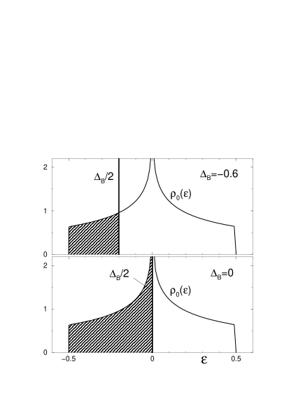
Figure 1: A schematic illustration of the two distinct critical fermion concentrations: (top) $n_{F}\simeq 0.4$ when boson energy $\Delta_{B}/2=-0.3$, and (bottom) $n_{F}=1$ when $\Delta_{B}/2=0$. The shaded areas show the occupied fermion states at zero temperature.

We take the boson fermion potential $g=0.1$ in all the results discussed below. Figure (2) shows the critical temperature $T_{c}$ of the $d$- wave superconducting phase for several values of $U$. This type of superconductivity is enhanced near the half-filled fermion system similarly as in the extended Hubbard model Ranninger-90 . In agreement to our expectations, the Coulomb repulsion only weakly reduces $T_{c}$ in a dilute fermion system. However, for $\Delta_{B}=0$ we notice a considerable reduction of $T_{c}$ or even a disappearance of superconductivity for $n_{F}=1$ (total concentration is then $n_{tot}=n_{F}+2n_{B}=2$) when $U$ exceeds the critical Mott transition value $U_{cr}$. For such a strong potential $U$ the $d$-wave superconducting phase is restricted to a narrower regime of the total concentration, such that there are no doubly occupied fermion states on a given lattice site (remember we are considering the intersite Cooper pairs).

Figure 2: Transition temperature $T_{c}$ into the $d$-wave superconducting phase as a function of the total concentration $n_{tot}$ for the two representative boson level values $\Delta_{B}=-0.6$ (top) and $\Delta_{B}=0$ (bottom). Curves corresponding to $U=0.1$ and $0.2$ where obtained from the mean field approximation, while $U=\infty$ from the salve boson study.

Figure (3) illustrates the effect of $U$ on the extended $s$-wave phase. In a dilute regime we notice almost identical values of $T_{c}$ for both the $d$- and extended $s$-wave superconducting phases. Also the influence of $U$ is there very similar. A remarkable difference appears for $\Delta_{B}=0$ when the fermion system is near the half-filling $n_{F}=1$. Critical temperature $T_{c}$ of the $s$-wave phase is then 3 times smaller as compared to the $d$-wave phase. The system is thus less susceptible for the $s$ type pairing near $n_{F}=1$ (for $\Delta_{B}=$ it corresponds to $n_{tot}=2$).

One notices also some ”peculiar” behavior of $T_{c}(n_{tot})$ for the extended $s$-wave phase cased by an increasing strength of $U$. With a small increase of $U$ the whole diagram is somewhat shifted and simultaneously the optimal value of $T_{c}$ slightly increases. This overall shift is caused by the Hartree term $Un_{F}/2$ (see the section III) which effectively pulls up the fermion band with respect to the boson energy level. By comparing the curves corresponding to $U=0$ in the upper and bottom panels of figure (3) we realize that such shift is responsible for enhancing the $s$-wave type superconductivity, but only when $U$ is safely smaller than $D$. A further increase of the Coulomb interaction $U$ proves to be detrimental on superconductivity (independently of a symmetry of the order parameter) because the fermion subsystem is driven into the Mott insulating state.

Figure 3: Transition temperature $T_{c}$ into the extended $s$-wave superconducting phase for several values of the on-site repulsion, as indicated. The top figure corresponds to $\Delta_{B}=-0.6$ and the bottom one to $\Delta_{B}=0$.

To analyze in more detail a pronounced effect of the Coulomb interaction on superconductivity for the half-filled fermion system $n_{F}=1$ ($n_{tot}=2$) we show in figure (4) the dependence of $T_{c}$ on $U$. The results have been obtained by means of the Alloy Analogy Approximation mentioned in section III and discussed earlier by the same author in Ref. TD_KIW-99 . For the $dim=2$ tight binding dispersion we determine the Mott transition at $U_{cr}\simeq 0.54$ in units of the initial fermion band. This value is probably underestimated. The most credible determination based on the dynamical mean field theory usually yields $U_{cr}$ larger than 1 DMFT-review . Nevertheless, a qualitative behavior presented in figure (4) remains valid. As we see by comparing to the figures (2,3) the AAA treatment properly interpolates between $U=0$ and $U=\infty$ limits.

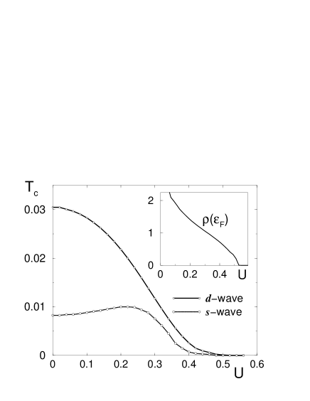
Figure 4: Transition temperature $T_{c}$ of the $d$- and the extended $s$-wave phases for the half-filled fermion system $n_{F}=1$. Both superconducting phases disappear when the Mott transition is approached. The inset shows the density of states at the Fermi energy for a normal phase obtained by the Alloy Analogy Approximation.

VII Conclusions

Summarizing, we have investigated the anisotropic superconductivity within the boson fermion model in a presence of the Coulomb repulsion between fermions.
(a) In a dilute regime of the fermion concentration the effect of the Coulomb repulsion proves to be rather weak. For both the $d$- and extended $s$-wave phase we observe up to 25 $\%$ reduction of the optimal $T_{c}$ value when $U\rightarrow\infty$. Both anisotropic phases survive, even in the limit of infinitely strong Coulomb repulsions.
(b) In the nearly half-filled fermion system we observe an enhancement of the $d$-wave superconducting phase and a simultaneous suppression of the $s$-wave phase until the interaction $U$ is small.
(c) Around the Mott transition $U_{cr}\simeq 0.54$ both phases are reduced to the concentration regime $n_{F}<1$, $2n_{B}<1$. Still, the superconductivity is able to survive at sufficiently large hole concentration $h=1-n_{F}>0$. Such a case is relevant for a description of the HTSC materials and boson fermion model seems to capable to reproduce qualitatively the phase diagrams known for these materials.

Among the problems which are not addressed in this paper there is a very intriguing question: what happens to pseudogap of the normal phase (discussed earlier in the Refs Domanski-01 ; perturbative ; Ren-98 ; DMFT and in Micnas-01 in a presence of Coulomb interactions ? Consideration of this subject is in a progress and the results shall be discussed elsewhere.

- (1) J. Ranninger and S. Robaszkiewicz, Physica B 135, 468 (1985).
- (2) G.M. Eliashberg, Pis’ma Zh. Eksp. Teor. Fiz. 46, 94 (1987).
- (3) R. Friedberg and T.D. Lee, Phys. Rev. B 40, 423 (1989); R. Friedberg, T.D. Lee and H.C. Ren, Phys. Lett. A 152, 417 (1991).
- (4) L. Ioffe, A.I. Larkin, Y.N. Ovchinnikov and L. Yu, Int. Journ. Modern Phys. B 3, 2065 (1989).
- (5) J. Ranninger and J.M. Robin, Physica C 253, 279 (1995).
- (6) M. Holland, S.J.J.M.F. Kokkelmans, M.L. Chiofalo and R. Walser, Phys. Rev. Lett. 87, 120406 (2001).
- (7) T. Kostyrko and J. Ranninger, Phys. Rev. B 54, 13105 (1996).
- (8) T. Domański and J. Ranninger, Phys. Rev. B 63, 134505 (2001).
- (9) T. Timusk and B. Statt, Rep. Prog. Phys. 62, 61 (1999).
- (10) J. Ranninger, J.M. Robin, M. Eschrig, Phys. Rev. Lett. 74, 4027 (1995); J. Ranninger and J.M. Robin, Solid State Commun. 98, 559 (1996); J. Ranninger and J.M. Robin, Phys. Rev. B 53, R11961 (1996); P. Devillard and J. Ranninger, Phys. Rev. Lett. 84, 5200 (2000).
- (11) H.C. Ren, Physica C 303, 115 (1998).
- (12) T. Domański, J. Ranninger and J.M. Robin, Solid State Commun. 105, 473 (1998).
- (13) J.M. Robin, A. Romano, J. Ranninger, Phys. Rev. Lett. 81, 2755 (1998); A. Romano and J. Ranninger, Phys. Rev. B 62, 4066 (2000).
- (14) H. Ding et al, Nature 382, 51 (1996); A.G. Loeser et al, Science 273, 325 (1996).
- (15) K.A. Kouznetsov et al, Phys. Rev. Lett. 79, 3050 (1997); A.G. Sun et al, Phys. Rev. Lett. 72, 2267 (1995).
- (16) J. Ma et al, Science 267, 862 (1995); H. Ding, J.C. Campuzano and G. Jennings, Phys. Rev. Lett. 74, 2784 (1995).
- (17) J. Betouras and R. Joynt, Europhys. Lett. 31, 119 (1995); K.A. Musaelian, J. Betouras, A.V. Chubukov and R. Joynt, Phys. Rev. B 53, 3598 (1996).
- (18) V.B. Geshkenbein, L.B. Ioffe and A.I. Larkin, Phys. Rev. B 55, 3173 (1997).
- (19) R. Micnas, S. Robaszkiewicz and B. Tobijaszewska, Physica B 312-313, 49 (2002); R. Micnas and B. Tobijaszewska, Acta Phys. Pol. B 32, 3233 (2001).
- (20) A. Romano, Phys. Rev. B 64, 125101 (2001).
- (21) T. Kostyrko, Acta Phys. Pol. A 91, 399 (1997).
- (22) G. Kotliar and A.E. Ruckenstein, Phys. Rev. Let. 57, 1362 (1986); D.H. Newns and N. Read, Adv. Phys. 36, 799 (1987).
- (23) T. Domański and K.I. Wysokiński, Phys. Rev. B 59, 173 (1999).
- (24) H. Schweitzer and G. Czycholl, Z. Phys. B 83, 93 (1991).
- (25) R. Micnas, J. Ranninger and S. Robaszkiewicz, Rev. Mod. Phys. 62, 113 (1990)
- (26) A. Georges, G. Kotliar, W. Krauth and M. Rozenberg, Rev. Mod. Phys. 68, 13 (1996).