Charge pumping in a quantum wire driven by a series of local time-periodic potentials

A parametric electron pump has attracted considerable attention in recent years. [1, 2, 3, 4, 5, 6, 7, 8, 9, 10, 11, 12] It is a device that generates a dc current at zero bias by cyclic deformations of system parameters.[1, 2, 3] The quantum pumping mechanism was originally proposed by Thouless,[1] who studied the integrated particle current produced by a slow periodic variation of the potential, and showed that in a finite torus the integral of the current over a period can vary continuously, but it must have an integer value in an infinite periodic system with full bands. Such quantized charge transport was proposed to become an electric current standard. [4]

Quite recently, the charge pumping was observed experimentally. [5] For technical reasons, instead of measuring charge currents, the pumped dc voltage $V_{dot}$ is measured in a quantum dot where two gates with oscillating voltages control the deformation of the shape of the dot. For weak pumping, the observed charge pumping has a sinusoidal dependence on the phase difference $\phi$ between the two shape-distorting ac voltages applied to the gates, and is proportional to the square of pumping strength $V$. For strong pumping, the pumped current deviates from the square dependence on $V$ and becomes nonsinusoidal, being always antisymmetric about $\phi=\pi$. The charge pumping may have a close relation to the adiabatic Berry’s phase since the evolution of the system is cyclic and is controlled by several system parameters, referred to as the parametric pumping. Based on this understanding, the total charge pumped per cycle is proportional to the area enclosed by the path in the parameter space, and nonzero pumping current requires at least two parameters. [5, 6] The pumped charge drived by two parameters should be zero if two parameters are in phase ($\phi=0$)) since the area enclosed by the path is zero. However, it is in contradiction with the observed current $I(\phi=0)\not=0$.[5] One of possible mechanisms of nonzero currents for $\phi=0$ is photovoltaic effects introduced in Ref.[2], where a surprising result, nonzero dc current generated by a single pumping gate voltage, is also reported. The general physics of a quantum pump has been the subject of several theoretical analyses.[2, 3] Zhou et al demonstrated that at low temperatures both the magnitude and the sign of the pumped charges are sample specific quantities, and the typical value in disordered (chaotic) systems turns out to be determined by quantum interference effects. Another general expression for the average transmitted charge current was derived by Brouwer [3] under the adiabatic condition and based on the time-dependent S-matrix method,[7] which appears to be quite successful for (adiabatic) weak pumping. Adiabaticity here means that the oscillating period $\tau$ of the system is much larger than the Wigner delay time $\tau_{w}$.[3, 8] Note that the adiabatic condition does not simply imply that the pumping strength $V$ should be very small. In fact, the adiabatic condition requires that $\tau$ must be larger as $V$ increases. On the other hand, the pumping was not weak in the experiments. [5] The main purpose of the paper is to develop a theory, which is also applicable in the case of strong pumping. By using the Floquet theorem, the photon-assisted transport has been taken into account[11]. We calculate the pumped current through a mesoscopic region in the presence of time-periodic potentials. Our main results in the weak pumping regime, as well as those in the strong pumping regime are consistent with the experiment reported in Ref.[5].

Consider electrons transmitting through a one-dimensional scattering region ranging from $x_{0}$ to $x_{0}+\delta$. The potential is given by

$$V(x,t)=\left\{\begin{array}[]{cc}0,&x_{0}<0,\ x>x_{0}+\delta\\ V_{s}(x,t),&x_{0}\leq x\leq x_{0}+\delta\end{array}\right.$$ (1)

with $V_{s}(x,t)=V_{0}+V_{s}cos(\omega t+\phi_{s})$. The Schrödinger equation can be written as

$$i\hbar\frac{\partial\Psi(x,t)}{\partial t}=-\frac{\hbar^{2}}{2m^{*}}\frac{\partial^{2}\Psi(x,t)}{\partial x^{2}}+V(x,t)\Psi(x,t),$$ (2)

with $m^{*}$ as the electron effective mass. Equation 2 can be solved by using the Floquet theorem.[13] By setting $\Psi_{Fl}(x,t)=e^{-iE_{Fl}t/\hbar}\psi(x,t),$ where $E_{Fl}$ is the Floquet eigenenergy and $\psi(x,t)$ is a periodic function $\psi(x,t)=\psi(x,t+\tau)$ with period $\tau=2\pi/\omega$, the Schrödinger equation takes the form

$$E_{Fl}\psi(x,t)=-\frac{\hbar^{2}}{2m^{*}}\frac{\partial^{2}\psi(x,t)}{\partial x^{2}}-i\hbar\frac{\partial\psi(x,t)}{\partial t}+V(x,t)\psi(x,t).$$

Substituting $\psi(x,t)=g(x)f(t)$, we have two separated equations with an introduced constant $E$,

$$-\frac{\hbar^{2}}{2m^{*}}\frac{\partial^{2}}{\partial x^{2}}g(x)+V_{0}g(x) = Eg(x),$$ (3)

$$i\hbar\frac{\partial f(t)}{\partial t}-V_{s}cos(\omega t+\phi_{s})f(t) = (E-E_{Fl})f(t).$$ (4)

Integrating Eq.(4) gives

$$f(t)=e^{\frac{iV_{s}sin\phi_{s}}{\hbar\omega}-\frac{i(E-E_{Fl})t}{\hbar}}\sum\limits_{\nu=-\infty}^{\infty}e^{-\nu\phi_{s}}J_{\nu}(\frac{V_{s}}{\hbar\omega})e^{-i\nu\omega t},$$ (5)

where $J_{\nu}(x)$ is the Bessel function of the first kind of order $\nu$. Since $f(t)$ is periodic in time with period $\tau$, it follows from Eq.(5) that $E-E_{Fl}=m\omega$ with $m$ as an integer. The equation for $g(x)$ has a solution

$$g(x)=e^{\pm ik^{s}_{m}x},\ (k^{s}_{m})^{2}=2m^{*}(E_{Fl}+m\hbar\omega-V_{0})/\hbar^{2}.$$ (6)

Thus $\psi(x,t)$ becomes

$$\psi_{m}(x,t)=e^{i(V_{s}/\hbar\omega)sin\phi_{s}\pm ik^{s}_{m}x}\sum\limits_{n}F_{n-m}e^{-in\omega t},$$ (7)

with $F_{n-m}=exp[-i(n-m)\phi_{s}]J_{n-m}(V_{s}/\hbar\omega)$.

We consider an incoming wave from the left with the energy $E_{0}=\hbar^{2}k_{0}^{2}/2m^{*}$, then the outgoing waves should be divided into different modes $E_{n}$, which satisfies $E_{n}=E_{0}+n\hbar\omega$ with $n=0,\pm 1,\pm 2,\cdots$. The propagating modes mean that $E_{n}>0$, while the evanescent modes mean that $E_{n}\leq 0$. The latter exists only in the neighborhood of the oscillating barrier and do not propagate. Denote $k_{n}=\sqrt{2m^{*}E_{n}}/\hbar$, the solutions of the Schrödinger equation can be written as

$$\Psi_{l} = \sum\limits_{n=-\infty}^{\infty}(A_{n}^{i}e^{ik_{n}x}+A_{n}^{o}e^{-ik_{n}x})e^{-iE_{n}t/\hbar},\ (x<x_{0})$$

$$\Psi_{s} = e^{-\frac{iE_{Fl}t}{\hbar}}\sum\limits_{m,n=-\infty}^{\infty}(a_{m}e^{ik^{s}_{m}x}+b_{m}e^{-ik^{s}_{m}x})F_{n-m}e^{-in\omega t},$$

$$( x_{0}\leq x\leq x_{0}+\delta)\$$

$$\Psi_{r} = \sum\limits_{n=-\infty}^{\infty}(B_{n}^{i}e^{-ik_{n}x}+B_{n}^{o}e^{ik_{n}x})e^{-iE_{n}t/\hbar},\ (x>x_{0}+\delta)$$

where $A_{n}^{i}$ and $B_{n}^{i}$ are the probability amplitudes of the incoming waves from the left and right, respectively, while $A_{n}^{o}$ and $B_{n}^{o}$ are those of the outgoing waves. We can characterize the barrier by a scattering matrix $S$ which is a matrix connecting the incoming and outgoing channels

$$\left(\begin{array}[]{c}{\bf A}^{o}\\ {\bf B}^{o}\end{array}\right)=S\left(\begin{array}[]{c}{\bf A}^{i}\\ {\bf B}^{i}\end{array}\right),$$

where the $S$ matrix can be derived by the matching conditions for the wave function $\Psi(x,t)$ and its derivative $\partial_{x}\Psi(x,t)$ at $x=x_{0}$ and $x=x_{0}+\delta$. After eliminating $a_{m}$ and $b_{m}$, we have [13]

$$S=\left(\begin{array}[]{cc}R_{\rightarrow}&T_{\leftarrow}\\ T_{\rightarrow}&R_{\leftarrow}\end{array}\right),$$ (8)

where $T_{\leftarrow}=L_{L}TL_{R}^{-1},$ $R_{\leftarrow}=L_{R}^{-1}{R}L_{R}^{-1},$ $T_{\rightarrow}=L_{R}^{-1}TL_{L},$ and $R_{\rightarrow}=L_{L}RL_{L}$. Here the left (right) arrow indicates incoming waves from right (left), the matrices $L_{L}$ and $L_{R}$ are defined as $(L_{L})_{mn}=exp[ik_{n}x_{0}]\delta_{mn}$ and $(L_{R})_{mn}=exp[ik_{n}(x_{0}+\delta)]\delta_{mn}$. $T$ and $R$ are given by

$$T = (C_{1}^{-1}D_{1}+C_{2}^{-1}D_{2})/2,$$ (9)

$$R = (C_{1}^{-1}D_{1}-C_{2}^{-1}D_{2})/2,$$ (10)

where

$$C_{1} = (L_{s}-\widetilde{I})K_{s}F^{\dagger}-(L_{s}+\widetilde{I})F^{\dagger}K,$$

$$D_{1} = -(L_{s}-\widetilde{I})K_{s}F^{\dagger}-(L_{s}+\widetilde{I})F^{\dagger}K,$$

$$C_{2} = (L_{s}+\widetilde{I})K_{s}F^{\dagger}-(L_{s}-\widetilde{I})F^{\dagger}K,$$

$$D_{2} = (L_{s}+\widetilde{I})K_{s}F^{\dagger}+(L_{s}-\widetilde{I})F^{\dagger}K,$$

with the matrices $(L_{s})_{mn}=exp[ik^{s}_{n}\delta]\delta_{mn}$, $(K_{s})_{mn}=k^{s}_{n}\delta_{mn}$, $K_{mn}=k_{n}\delta_{mn}$, $\widetilde{I}$ as the unit matrix and $F^{\dagger}$ as the Hermitian conjugate of $F$. The electronic transport properties of the scattering region may be obtained straightforward from Eq.(8).

The above method may be generalized to $l$ time-periodic barriers described by

$$V(x,t)=\left\{\begin{array}[]{cc}0,&x<0,\ x>a_{l}\\ V_{1}(x,t),&0\leq x<a_{1}\\ V_{2}(x,t),&a_{1}\leq x<a_{2}\\ \vdots&\vdots\\ V_{l}(x,t),&a_{l-1}\leq x\leq a_{l}\end{array}\right.$$ (11)

where $V_{1}(x,t)=V_{1}^{0}+V_{1}cos(\omega_{1}t+\phi_{1})$, $V_{2}(x,t)=V^{0}_{2}+V_{2}cos(\omega_{2}t+\phi_{2}),\cdots$ and $V_{l}(x,t)=V^{0}_{l}+V_{l}cos(\omega_{l}t+\phi_{l})$. This potential may be more a realistic model for experiments. Obviously the transport properties for each barrier can be characterized by an $S$ matrix given by

$$S^{\alpha}=\left(\begin{array}[]{cc}R_{\rightarrow}^{\alpha}&T_{\leftarrow}^{\alpha}\\ T_{\rightarrow}^{\alpha}&R_{\leftarrow}^{\alpha}\end{array}\right),$$

where $\alpha=1,2,\cdots,l$, $T_{\rightarrow}^{\alpha}$, $T_{\leftarrow}^{\alpha}$, $R_{\rightarrow}^{\alpha}$ and $R_{\leftarrow}^{\alpha}$ can be derived by the same method presented above. Now the propagating mode $E_{n}$ should be replaced by

$$E(n_{j})=E_{0}+\sum\limits_{n_{j}=-\infty}^{\infty}n_{j}\hbar\omega_{j}.\ \ (j=1,\cdots,l)$$ (12)

The associated transfer-matrix $M^{\alpha}$ for the $\alpha$th barrier may be derived directly from the $S^{\alpha}$ matrix

$$M^{\alpha}=\left(\begin{array}[]{cc}(T_{\leftarrow}^{\alpha})^{-1}&-(T_{\leftarrow}^{\alpha})^{-1}R_{\rightarrow}^{\alpha}\\ R_{\leftarrow}^{\alpha}(T_{\leftarrow}^{\alpha})^{-1}&T_{\rightarrow}^{\alpha}-R_{\leftarrow}^{\alpha}(T_{\leftarrow}^{\alpha})^{-1}R_{\rightarrow}^{\alpha}\end{array}\right).$$

The total transfer-matrix $M^{t}$ for all those barriers is determined by

$$M^{t}=\left(\begin{array}[]{cc}M_{11}^{t}&M_{12}^{t}\\ M_{21}^{t}&M_{22}^{t}\end{array}\right)=M^{l}M^{n-l}\cdots M^{1},$$

where $M^{t}_{ij}\ (i,j=1,2)$ are the partitioned matrices with the same size as $T^{\alpha}_{\rightarrow}$. The total scattering matrix $S^{t}$ can be derived from $M^{t}$ as

$$S^{t}=\left(\begin{array}[]{cc}-(M_{11}^{t})^{-1}M_{12}^{t}&(M_{11}^{t})^{-1}\\ M_{22}^{t}-M_{21}^{t}(M_{11}^{t})^{-1}M_{12}^{t}&M_{21}^{t}(M_{11}^{t})^{-1}\end{array}\right).$$

In each cycle a net charge current may pass through the scattering region in the direction determined from the detailed form of $S^{t}$ matrix. We define a net transmission coefficient (for an incoming wave in mode $E_{0}=E$) by

$$T_{net}=\sum\limits_{E(n_{j})>0}\sqrt{\frac{2E(n_{j})}{m^{*}}}(|T^{t}_{\rightarrow,n_{j}0}(E_{0})|^{2}-|T^{t}_{\leftarrow,n_{j}0}(E_{0})|^{2}).$$

The average net current per period $\tau$ (for $E_{0}$) through those barriers is $j(E_{0})=T_{net}(E_{0})$. If the system is connected through two ideal leads to two electron reservoirs with the same chemical potential $\mu$, the average pumped current per period $\tau$ is given by [13, 14]

$$I(\mu)=e\int_{0}^{\infty}dEg(E)f(E-\mu)T_{net}(E),$$ (13)

where $g(E)=\sqrt{2m^{*}/E}/h$ is the density of electrons contributing to the current in one direction, and $f(E-\mu)$ is the Fermi-Dirac distribution. At zero temperature, it becomes

$$I(\mu)=\frac{2e}{h}\int_{0}^{\mu}dE\sqrt{\frac{m^{*}}{2E}}T_{net}(E).$$ (14)

Another important quantity is the Wigner delay time which gives the time delay of the scattered electron due to its interaction with the scattering field ( here the oscillating potential). It relates to the S-matrix by [15]

$$\tau_{w}(E)=-\frac{i\hbar}{N_{c}}Tr[(S^{t})^{\dagger}\frac{dS^{t}}{dE}]=-\frac{i\hbar}{N_{c}}\frac{d}{dE}ln(detS^{t}),$$ (15)

where $N_{c}$ is the number of open channels. Physically, the Wigner time represents the time spent by a wave packet passing through the scattering region. The charge pumping is supposed to be adiabatic when $\tau$ is much greater than the Wigner delay time $\tau_{w}$.

It is obvious that the net charge transfer in one cycle is zero for a single time-periodic barrier since $T_{\rightarrow}=T_{\leftarrow}$. Then the simplest system which may induce the nontrivial charge pumping should include at least two barriers. As an example we consider a mesoscopic system with two time-periodic barriers connected through ideal leads to two electron reservoirs with the same chemical potentials $\mu$. The potentials are described by $V_{1}(x,t)=V_{1}^{0}+V_{1}cos(\omega t)$, $V_{2}(x,t)=V_{2}^{0}$, and $V_{3}(x,t)=V_{3}^{0}+V_{3}cos(\omega t+\phi)$. This appears to be a simplified model for the Switkes et al’s experiment, nevertheless it turns out that some essential characteristics can be exhibited, as we will address below. In the following numerical calculations, $\mu=75\ mev$, $m^{*}=0.067m_{e}$ (with $m_{e}$ as the mass of the free electron), $V_{2}^{0}=-30\ mev$, $V_{2}=0$, and $N_{c}$ is determined by a natural condition: $|T_{\rightleftharpoons}|^{2}+|R_{\rightleftharpoons}|^{2}-1.0\leq c_{e}$ with $c_{e}$ ($=1.0\times 10^{-4}$ in this paper) as a defined error.

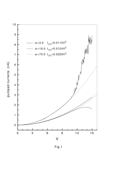
FIG. 1.: The pumped currents $I(\phi=\pi/2)$ versus the barrier height $V$ for different pumping frequencies. Dotted lines fit the relation $I_{(V)}\propto V^{2}$.

The general characteristics of quantum pumping are shown in Figs.1 and 2. The parameters in Figs.1, 2, and 3 are chosen as $V^{0}_{1}=V^{0}_{3}=50\ mev$, and $V_{1}=V_{3}=V$. Figure 1 shows that the pumped current $I(V)$ is proportional to $V^{2}$ for small pumping amplitude $V$, with the proportional factor depending on the driving frequency ($\hbar=1$). But it deviates from $V^{2}$-dependence for the strong pumping case. On the other hand, the pumped current is sinusoidal dependence on $\phi$ for weak pumping, and becomes nonsinusoidal dependence on $\phi$ when $V$ increases, as seen in Fig.2. Another important characteristic shown in Fig.2 is that $I(\pi+\phi,V)=-I(\phi,V)$ for all amplitude strengths, and $|I(\phi,V)|$ is maximum at $\phi=\pi/2$ or $\phi=3\pi/2$ for weak pumping. Remarkably, these results for $I(\phi,V)$ are in agreement with the experimental observation in Ref.[3].

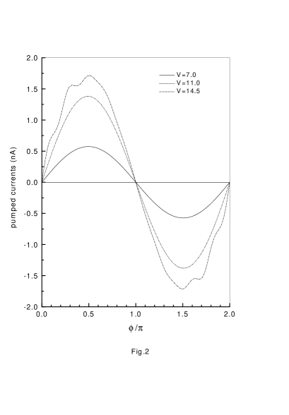
FIG. 2.: The pumped currents versus the phase difference $\phi$ for three different $V$ and $\omega=3.0$.

Figure 3 shows that sharp peaks in the Wigner time occur at the resonance insert energies $E_{0}=n\hbar\omega$. Besides, jumps in the pumped current as a function of $E_{0}$ appear at the peak positions of the Wigner time. The direction of the current depends crucially on the insert energy. It is interesting to note that the adiabatic condition is not necessary in our calculations. Figure 3 indicates that the maximum value of $\tau_{w}$ is about $5.5\ ns$ for $\hbar\omega=6.0\ mev$ (corresponding to $\tau\sim 0.7\ ps$ ), which is much greater than the pumping cyclic time $\tau$. Then we may say that the method described here is beyond adiabaticity. Actually, the nonadiabatic effects are only important for the strongly photon-assisted transport since $\tau_{w}$ is greater than $\tau$ only if the energy of the incoming wave is approximately equal to the resonance energy for photon-assisted tunneling. Physically, by emitting or absorbing photons, the outgoing waves may be at the quantum states different from that of the incoming wave. Consequently, the adiabatic condition, which requires that the quantum state is at the same instant state in the whole evolution, is not satisfied. Note that the formula derived by Brouwer[3] may be valid merely under the adiabatic condition, and thus the method developed here may be quite useful.

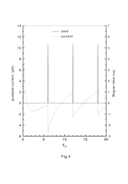
FIG. 3.: The pumped current and the Wigner delay time versus the insert energy $E_{0}$ for $V=7.0$ and $\omega=6.0$.

It is quilt intriguing to note from Fig.4 that $I(\phi=0)$ is nonzero for $V_{1}\not=V_{3}$, while the corresponding areas enclosed by the path in the parameter space $\{V_{1}(x,t),V_{3}(x,t)\}$ are zero. Although the pumped currents in the above case were predicated to be zero under the adiabatic approximation, the deviation from zero is reported experimentally at strong pumping,[5] just as we observed here in terms of a rigorous theoretical analysis which is also valid for strong pumping. Moreover, from comparison with that $I(\phi=0)=0$ for $V_{1}=V_{3}$, it is now clear that the present nonzero pumped currents stem from the spatial asymmetry of potentials $V_{1}\not=V_{3}$, which is coincident with the result obtained by Wagner in Ref.[11]: the nonzero currents may be observed in a single osscillating potential but with asymmetric static potential. Actually, to observe a pump current at zero applied bias, it seems that the inversion symmetry should be broken, either in real or in $k$ space.

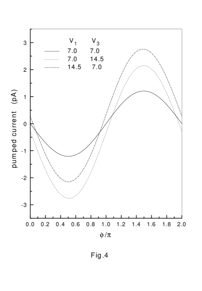
FIG. 4.: The pumped currents versus the phase difference $\phi$ for $\omega=3.0$ for different $V_{1}$ and $V_{3}$.

The fact that $I(\phi=0)$ is nonzero at strong pumping may be understood based on a scenario of the nonadiabatic geometric phase.[16] Pumped currents are determined by geometric phase accumulated in the evolution. [1, 5, 6] Under the adiabatic approximation, $I(\phi=0)=0$ is predicted theoretically because the corresponding adiabatic geometric phase is zero. While it is now clear that the nonadiabatic geometric phase may be nonzero even in the case where the area enclosed by the path in the parameter space is zero (thus the adiabatic phase is zero).[16] Therefore, the nonadiabatic correction to the currents should be taken into account for strong pumping whenever the adiabatic condition is not well satisfied. Physically, it is reasonable to believe that the observed nonzero pumping at phase $\phi=0$ for the strong pumping stems from the nonadiabatic correction when the inversion symmetry is broken. Practically, the asymmetric spatial potential might be present in the experiment, which may originate from either the shape-distorting ac voltages, or from the internal potential established during transport.[7] Since the current calculated in this approach is conserved since $|T_{\rightleftharpoons}|^{2}+|R_{\rightleftharpoons}|^{2}=1.0$, no internal potential appears explicitly in the present formulism. It is worth pointing out that nonzero pumped currents for $\phi=\pi$ are also seen in Fig.4, which seems to contradict with that in Ref [5]. Also note that a nonzero $I(\phi=\pi)$ was also predicted by another totally different theoretical study[17], so this contradication is still an interesting open question at present.

In summary, we developed a method to calculate the pumped current and Wigner delay time in a mesoscopic system with a series of time-periodic barriers connected to two electron reservoirs, which appears to be applicable for strong pumping cases.

We thank the support from a RGC grant of Hong Kong(Grant No. HKU7118/00P) and a CRCG grant at the University of Hong Kong.

REFERENCES

[1] D. J. Thouless, Phys. Rev. B 27, 6083 (1983).
[2] F. Zhou, B. Spivak, and B. Altshuler,
Phys. Rev. Lett. 82, 608 (1999).
[3] P. W. Brouwer, Phys. Rev. B 58,
R10135 (1998).
[4] Q. Niu, Phys. Rev. Lett. 64, 1812 (1990).
[5] M. Switkes, C. M. Marcus, K. Campman, and A. C.
Gossard, Science, 283, 1905 (1999).
[6] B. L. Altshuler and L. I. Glazman, Science,
283, 1864 (1999).
[7] M. Büttiker, H. Thomas, and A. Prêtre,
Z. Phys. B 94, 133 (1994).
[8] A. Andreev and A. Kamenev,
cond-mat/0001460.
[9] I. L. Aleiner and A. V. Andreev,
Phys. Rev. Lett. 81, 1286 (1998);
T. A. Shutenko, I. L. Aleiner, and B. L. Altshuler,
Phys. Rev. B 61, 10 366 (2000).
[10] Y. Levinson, O. Entin-Wohlman, and P. Wölfle,
Phys. Rev. Lett. 85, 634 (2000).
[11] M. Wagner, Phys. Rev. Lett. 85, 174 (2000);
M. Wagner and F. Sols, ibid. 83, 4377 (1999);
M. Wagner, ibid.76, 4010 (1996).
[12] Y. Wei, J. Wang, and H. Guo, Phys. Rev. B 62, 9947 (2000).
[13] G. Burmeister and K. Maschke, Phys. Rev.
B 57, 13 050 (1998); W. Li and L. E. Reichl,
ibid.60, 15 732 (1999).
[14] R. Landauer, Philos. Mag. 21, 863 (1970);
M. Büttiker, Phys. Rev. Lett. 57, 1761 (1986).
[15] E. P. Wigner, Phys. Rev. 98, 145 (1955);
F. T. Smith, ibid.118, 349 (1960).
[16] S. L. Zhu and Z. D. Wang, Phys. Rev. Lett. 85, 1076 (2000);
S. L. Zhu, Z. D. Wang, and Y. D. Zhang, Phys. Rev. B 61, 1142 (2000).
[17] B. Wang, J. Wang, and H. Guo, Phys. Rev. B,
073306 (2002).