Conductance of a quantum point contact in the presence of spin-orbit interaction

I Introduction

The interaction between the electron spin and its orbital motion, commonly refered to as the spin-orbit (SO) interaction or SO coupling, has been known for a long time. Recently the effect of SO-interaction on mesoscopic transport phenomena and the quantum Hall effect has attracted growing interest. [1, 2, 3, 4, 5, 6, 7, 8] Although the interaction magnitude is small compared to the Fermi energy, it may have significant impact on electronic transport, particularly in mesoscopic systems where quantum interference is extremely important. Using the transfer matrix method, Meir et al. [1] showed that the SO-interaction in one-dimensional (1D) non-interacting disordered rings induces an effective spin-dependent magnetic flux, and then any spin-dependent transport quantity can be expressed in terms of the same quantity in the absence of the SO scattering but with an effective magnetic flux. The adiabatic Berry phase induced by the SO-interaction and its effect on the electronic transport were studied extensively by Loss et al., [2] Aronov and Lyanda-Geller. [3] Persistent currents in mesoscopic rings induced by the SO-interaction was addressed in Ref.4. Promisingly, as observed by Morpurgo et al., [6] the geometric phase induced by the SO-interaction [1, 2, 3, 4, 5] could induce the splitting of the main peak in the ensemble average Fourier spectrum. Also interestingly, lifting of the spin degeneracy by the Rashba SO-interaction[9] was reported experimentally in two-dimensional (2D) electron systems for different semiconductor structures. [10] Lommer et al. pointed out that the Rashba mechanism becomes dominant in a narrow gap semiconductor system. [11] The spin splitting energy at the Fermi energy in the absence of magnetic field is $\Delta=2\alpha k_{F}$ (with $\alpha$ as a SO coupling constant and $k_{F}$ as the Fermi wave vector), which is about $1.0\sim 5.0\ meV$ in typical semiconductor materials. [10]

On the other hand, the observation of the universal [12, 13] and the nonuniversal [14] quantizations of the conductance in a quasi-1D constrication is also remarkable. In a clean quasi-1D constrication, if the mean free path is much longer than the effective channel length, the conductance is quantized in unit of $2G_{0}$ with $G_{0}=e^{2}/h$ at zero magnetic field, referred to as the universal quantization, where the factor of $2$ aries from the electron spin degeneracy. [12, 13] Recently, Thomas and co-workers found that, in addition to the above quantized conductance plateau, there is also a structure at $0.7(2G_{0})$. This so-called $0.7$ structure (nonuniversal or fractional conductance quantization) appears to be related to spontaneous lifting of spin degeneracy in the 1D constrication, but the origin of it remains as an open question. [14] Since the $0.7$ structure may be understood as a zero-field spin splitting with an estimated energy of $\Delta\sim 1meV$, [14] which is the same order as the spin splitting energy induced by the SO-interaction, it is nature to ask an important question: Is the spin polarization induced by the SO coupling responsible for the $0.7$ structure? To answer this question, we study the effect of SO-interaction on the electronic transport through quantum point contacts (QPC) in this paper. We find that the $0.7$ structure is unlikely to stem from the SO-interaction. However, some interesting oscillations in the ‘quantized’ conductance may be induced by the SO-interaction, and may be experimentally observable. Moreover, the spin-dependent transport properties are of current interest in both fundamental physics and applied spin electronics. It is quit intriguing to develop a method to calculate the spin-dependent transport in mesoscopic systems. Also in this paper, generalizing a method established for spin-independent cases [15, 16] we have done such a job. It is worth pointing out that another theoretical approach[17] may be generalized to calculate the spin-dependent conductance.

The paper is organized as follows. In Sec.II A, we derive the 2D tight-binding Hamiltonian with the Rashba SO coupling. In Sec.II B, the recursive Green’s function technique is presented to calculate the spin-dependent transmission coefficient. In Sec.III the conductance is calculated numerically in a model QPC in the presence of SO coupling and/or magnetic field. The finite temperature effect is also studied. This paper ends with a brief summary.

II Model and calculation method

A 2D tight-binding Hamiltonian with the Rashba SO coupling

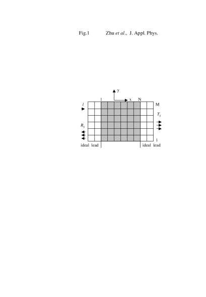
FIG. 1.: Schematic diagram of the system. Electrons are injected from the left lead.

In a magnetic field, the 2D Hamiltonian for electrons (of effective mass $m^{*}$ and charge $e$) with the Rashba SO-interaction reads [9]

$$H=\frac{{\bf\Pi}_{x}^{2}+{\bf\Pi}_{y}^{2}}{2m^{*}}+\frac{\alpha}{\hbar}(\hat{\sigma}_{x}{\bf\Pi}_{y}-\hat{\sigma}_{y}{\bf\Pi}_{x})+U(x,y)-\frac{g\mu_{B}}{2}{\stackrel{{\scriptstyle\hat{\rightarrow}}}{{\sigma}}}\cdot{\bf B},$$ (1)

where ${\bf\Pi}={\bf p}-\frac{e}{c}{\bf A}$ is the canonical momentum, $U(x,y)$ represents the spin-independent potential, ${\bf A}$ is the electromagnetic gauge potential with ${\bf B}=\nabla\times{\bf A}$ relating it to the magnetic fields, and $g$, $\mu_{B}$,${\stackrel{{\scriptstyle\hat{\rightarrow}}}{{\sigma}}}$ are the $g$ factor, Bohr magneton, Pauli matrices respectively. $\alpha$ is the Rashba SO-interaction constant which is determined from an effective electric field along $z$ direction given by the form of the confining potential in the absence of an inversion center. Now we choose a discrete square lattice, on which points are located at $x=na$ and $y=ma$, with $n,m$ as integers and $a$ as the lattice constant. In terms of the quaternion, the one-electron tight-binding Hamiltonian with the Rashba SO coupling can now be parameterized as

$$H = \sum\limits_{nm}\varepsilon_{nm}|nm\rangle\langle nm|-\sum\limits_{nm}(V_{nm,n-1m}|nm\rangle\langle n-1m|$$ (2)

$$+ V_{nm,nm-1}|nm\rangle\langle nm-1|+H.C.),$$ (3)

where $|nm\rangle$ is a two-component orthonormal set in the lattice sites $(n,m)$; $\varepsilon_{nm}=(U_{nm}+4t)\tau_{0}-i\gamma\tau_{3}$ with $U_{nm}=U(x=na,y=ma)$, $t=\hbar^{2}/2m^{*}a^{2}$, $\gamma=g\mu_{B}B_{z}/2$; $V_{nm,n-1m}=V_{x}exp(-ieA_{x}a/\hbar)$ and $V_{nm,nm-1}=V_{y}exp(-ieA_{y}a/\hbar)$ with $V_{x}=t\tau_{0}-\alpha^{\prime}\tau_{2}$, $V_{y}=t\tau_{0}+\alpha^{\prime}\tau_{1}$ and $\alpha^{\prime}=\alpha/2a$. The quaternion basis $\{\tau_{i}\}$ is defined by the $2\times 2$ unit matrix $\tau_{0}$ and $\tau_{l}=-i\hat{\sigma}_{l}\ (l=1,2,3)$ with $\hat{\sigma}_{l}$ as the Pauli matrices. $A_{x}$ or $A_{y}$ is evaluated at the middle point between sites $(n,m)$ and $(n+1,m)$ or $(n,m+1)$.

B Model and the recursive Green’s function technique

To describe spin-dependent transport properties through a specific mesoscopic structure, we consider a 2D structure composed of three different regions ( Fig.1). The shadowed central zone is a mesoscopic structure where the SO coupling and/or a homogeneous perpendicular magnetic field are present. To simplify scattering boundary conditions, we assume that the structure is connected to both sides with semi-infinite ideal leads without SO-interaction and magnetic field. In our lattice model atoms are at the sites of a square lattice $(na,\ ma)$ ( with $a$ to be set equal to unit, $m=1,2,\cdots,M$.) in the shadowed zone and two ideal leads. As a result the system is described by a one-electron tight-binding Hamiltonian similar to Eq.(3). For a homogeneous magnetic field ${\bf B}=(0,\ 0,\ B)$ perpendicular to the 2D-plane (${\bf A}=(-yB,\ 0,\ 0)$ in the Landau gauge), we can write the Hamiltonian for the shadowed central zone as

$$H_{c}=\sum\limits_{n=1}^{N}|n)H_{n}(n|+\sum\limits_{n=1}^{N-1}[|n)H_{n,n+1}(n+1|+H.C.],$$ (4)

where $|n)$ is the set of $2M$ ket vectors belonging to the $n$th cell, and

$$H_{n}\equiv H_{n,n}=\left(\begin{array}[]{lllll}\varepsilon_{n1}&-V_{y}^{+}&0&\cdots&0\\ -V_{y}&\varepsilon_{n2}&-V_{y}^{+}&\cdots&0\\ 0&-V_{y}&\varepsilon_{n3}&\cdots&0\\ \vdots&\vdots&\vdots&\ddots&\vdots\\ 0&0&0&\cdots&\varepsilon_{nM}\end{array}\right),$$ (5)

$$(H_{n,n+1})_{pp^{\prime}}=-V_{x}^{+}e^{-i2\pi\beta(p-\frac{M+1}{2})}\delta_{pp^{\prime}}\ \ (p,p^{\prime}=1,\cdots,M).$$ (6)

Here $\beta=Ba^{2}/\phi_{0}$ with $\phi_{0}=hc/e$ as the magnetic flux quantum. The forms of Hamiltonian for the two ideal leads are the same as Eq.(4), but with different summing regions ($-\infty<n<1$ at the left lead and $N<n<\infty$ at the right lead) and different values of the parameters: $V_{x}=V_{y}=t\tau_{0},\ \ \varepsilon_{nm}=4t\tau_{0},\ \ B=0$. Moreover, it seems acceptable to assume that the coupling between the ideal leads and the mesoscopic structure takes simply the form $H_{0,1}=H_{N,N+1}=-t\delta_{pp^{\prime}}$. [18]

Following the recursive Green’s function technique developed for some spin-independent systems, [15, 16, 19] we may generalize the method to the nontrivial spin-dependent cases. The spin-dependent transmission $t_{lj}^{\sigma\sigma^{\prime}}$ for the incident channel $(l,\sigma)$ and out-going channel $(j,\sigma^{\prime})$ can be found readily (see the appendix A) . At a finite temperature $T$, the conductance through a 2D mesoscopic structure is given by the Landauer-Büttiker formula [20]

$$G=-G_{0}\sum\limits_{lj,\sigma\sigma^{\prime}}\int_{0}^{\infty}T^{\sigma\sigma^{\prime}}_{lj}\frac{\partial f(E,T)}{\partial E}dE,$$ (7)

where $T^{\sigma\sigma^{\prime}}_{lj}=|t^{\sigma\sigma^{\prime}}_{lj}|^{2}$ is determined from Eq.(A3), and $f(E,T)=[1+exp(E-E_{f})/k_{B}T]^{-1}$ is the Fermi-Dirac distribution function with $k_{B}$ as the Boltzmann constant. Obviously, Eq (7) reduces to $G=G_{0}\sum_{\{lj,\sigma\sigma^{\prime}\}}T^{\sigma\sigma^{\prime}}_{lj}$ at zero temperature.

In the following, we focus on a QPC structure with the Büttiker saddle-point potential

$$U_{nm}=V_{0} - \frac{1}{2}m^{*}\omega_{x}^{2}a^{2}[n-(N+1)/2]^{2}$$ (8)

$$+ \frac{1}{2}m^{*}\omega_{y}^{2}a^{2}[m-(M+1)/2]^{2},$$ (9)

which is a practical candidate to describe a real QPC. [21] $\omega_{x,y}$ indicate the strength of the lateral confinement. Note that the well-pronounced quantized plateaus occur if $\omega_{y}\geq\omega_{x}$.

Before the end of this section, it is worth pointing out that the recursive Green’s function method described in this section can be straightforwardly generalized to 3D mesoscopic structures, and thus is quite useful in studying the spin-dependent transport of many different mesoscopic structures which are of current interest, such as the devices with quantum Hall effect, giant magnetoresistance, tunnel magnetoresistence.

III Numerical results

We now calculate numerically the conductance of the QPC in the presence of SO-interaction and/or a magnetic field. We here present the results for the system of $M=7$, $N=15$ [22] and $t=1$.

A The effects of SO interaction

It is well known that the conductance through QPC is quantized with the unit of $2G_{0}$ as a function of the saddle energy $V_{0}$. The conductance quantization is well explained by Landauer-Büttiker formula of quantum ballistic transport: for a nonmagnetic QPC, the spin-up and spin-down electrons make the same contribution and then the unit of the conductance quantization is $2G_{0}$. However, if the Rashba SO-interaction is present in the QPC, the spin degeneracy of conductance electrons would be broken. Whether the quantization of the conductance is affected by the SO-interaction in a meaningful sense?

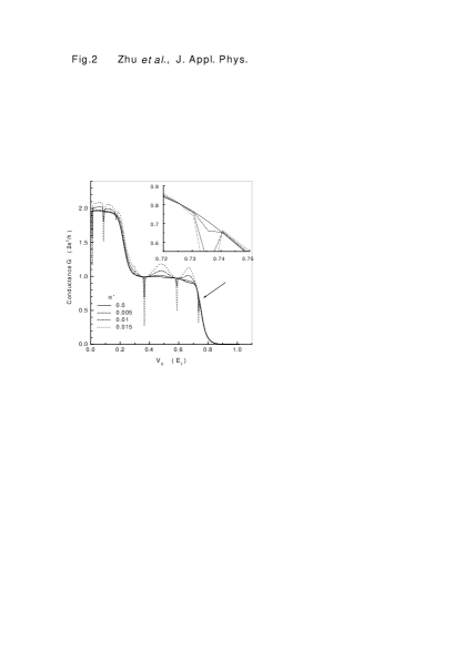
FIG. 2.: The conductance $G$ versus the saddle energy $V_{0}$ ( in unit of $E_{f}$) in the presence of SO-interaction for $\beta=k_{B}T=0$, $E_{f}=1.21$, $\omega_{y}=3\omega_{x}$. The inset shows an enlargement of the curve around the arrow.

Figure 2 shows the conductance $G$ as a function of $V_{0}$ for the SO parameters $\alpha^{\prime}=0,$ $0.005$, $0.01$, and $0.015$. Other parameters are $E_{f}=1.21$, $\omega_{y}=3\omega_{x}$. Two effects of the SO-interaction on the conductance are seen. (i) The SO-interaction induces some oscillations on the plateaus, and the stronger the SO-interaction is the larger the oscillation amplitude is. Remarkably, some sharp dips exist on the oscillation for the strong SO coupling, for example, the height of dip is almost $2G_{0}$ for $\alpha^{\prime}\sim 0.015$. (ii) A tiny plateau exists near $0.7(2G_{0})$ for a weak SO interaction $\alpha\sim 0.005$ ( We will address the temperature effect on this tine plateau later). But it becomes a sharp dip for the strong SO-interaction (see the inset of Fig.2). The conductance oscillations as well as the sharp dips in the plateaus may be observable in future mesoscopic experiments.

We now attempt to understand the above numerical results heuristically. The conductance oscillations appear to stem from the multiple reflections with the SO coupling. By taking into account the multiple reflections, the conductance of the QPC may be rewritten as [12]

$$G=G_{0}\sum\limits_{j\sigma}\frac{(1-R_{j\sigma})^{2}}{1-2R_{j\sigma}cos(2k_{j\sigma}L_{x})+R_{j\sigma}^{2}},$$ (10)

where the reflection probability $R_{j\sigma}$ for channel $(j,\sigma)$ is given by

$$R_{j\sigma}=\left(\frac{v^{L}_{j}-v^{c}_{j\sigma}}{v^{L}_{j}+v^{c}_{j\sigma}}\right)^{2},$$ (11)

with $v^{L}_{j}$ ( $v^{c}_{j\sigma}$) as the value of velocity in the leads ( scattering zone). $v^{c}_{j\sigma}=\partial E^{c}_{j\sigma}/\hbar\partial k$ is determined by the dispersion relation for the electron states in the QPC, which is approximately written as

$$E^{c}_{j}\approx\hbar^{2}k_{j}^{2}/2m^{*}+(j-1/2)\hbar\omega_{y}+V_{0}$$ (12)

(independent on $\sigma$) in the absence of the SO coupling,[12] but as

$$E^{c}_{j\sigma}\approx\hbar^{2}k_{j\sigma}^{2}/2m^{*}+\sigma\alpha|k_{j\sigma}|+(j-1/2)\hbar\omega_{y}+V_{0}$$ (13)

in the presence of SO coupling. Here we only consider the energy spectrum at $x=0$ since the transport properties for the Büttiker saddle-point potential depend mainly on the narrowest part. Note that the quantized plateaus are well-pronounced in the absence of the SO coupling (as shown in Fig.2) since $v^{c}_{j}=\hbar^{2}k_{j}/m^{*}\sim v^{L}_{j}$ and thus $R_{j}$ for a propagating model in the Büttiker saddle-point potential is negligible. However, the additional $R_{j\sigma}$ may be induced from the SO coupling because as seen from Eq.(13) $v^{c}_{j\sigma}$ in the presence of SO coupling is different from that in the absence of SO coupling. Therefore, the oscillations may stem from the SO coupling since Eq (10) predicts the transmission oscillations, provided that $R_{j\sigma}$ induced by the SO coupling are not too small. [23] Moreover, we can understand from Eqs. (10) and (11) that a dip in the conductance may appear for a relatively larger $R_{j\sigma}$ when an electron in the channel $(j,\sigma)$ is in a propagating state ($k_{j\sigma}>0$) with $v^{c}_{j\sigma}\sim 0$. It is interesting to note from Eq.(13) that $v^{c}_{j-}=0$ for $\tilde{k}_{j}=m^{*}\alpha/\hbar^{2}$, which corresponds the minimum of $E^{c}_{j\sigma}$ as a function of momentum. When $V_{0}$ varies in the scale of magnitude $\sim\alpha\tilde{k}_{j}$, $v_{j}^{c}\sim 0$ for the same $v_{j}^{L}$-channel as in the absence of SO coupling. This clearly shows that a larger $R_{j\sigma}$ may appear in a narrow region in the presence of the SO coupling, leading to a dip. Our numerical results in Fig.2 agree qualitatively with the above arguments.

We now look into whether the interesting behaviors seen in Fig.2 are sensitive to the set of parameters. Firstly, we plot Fig.3(a) and (b) for two other different $\omega_{y}/\omega_{x}$ ( the other parameters are the same as those in Fig.2). The plateaus are not well pronounced for $\omega_{y}=1.5\omega_{x}$ even if $\alpha^{\prime}=0$(Fig.3(a)). In this case, the SO-induced oscillations are not so distinctive with the conductance curve for $\alpha^{\prime}=0$, but the sharp dips still appear in the conductance. For $\omega_{y}=6\omega_{x}$ ( Fig.3(b)), the width of the plateaus is widened. Comparing the results in Fig.2, Fig.3(a), and (b), we found that the well-pronounced plateaus occur for larger ratio $\omega_{y}/\omega_{x}$, which is due to the Büttiker saddle-point potential. We also noticed that the effects induced by the SO coupling are similar to those in Fig.2. Secondly, we plot Fig.3(c) and (d) for two other different Fermi energies (the other parameters are the same as those in Fig.2). It is seen that the main effects induced by the SO coupling are still similar to those in Fig.2. Therefore, we may conclude that the essential feature induced by the SO coupling in Fig.2 is not quite sensitive to the Fermi energy and the ratio of $\omega_{y}/\omega_{x}$, but is indeed sensitive to the SO coupling parameter $\alpha^{\prime}$.

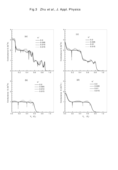
FIG. 3.: The conductance $G$ versus the saddle energy $V_{0}$ in the presence of SO-interaction for $\beta=k_{B}T=0$. (a) $E_{f}=1.21$, $\omega_{y}=1.5\omega_{x}$; (b) $E_{f}=1.21$, $\omega_{y}=6\omega_{x}$; (c) $E_{f}=2.0$, $\omega_{y}=3\omega_{x}$; (d) $E_{f}=1.0$, $\omega_{y}=3\omega_{x}$.

The temperature dependence of the conductance as a function of $V_{0}$ can be seen from Figs.4(a) and (b). Firstly, in certain temperature regions, the oscillation induced by the SO-interaction disappears when the temperature increases, meanwhile the quality of the quantized plateaus is improved. However the quantized plateaus are destroyed when temperature increases further. The mechanism for the destruction of the quantized plateaus by the finite temperature is energy averaging.[12] Secondly, the tine plateau and the dip near $0.7(2G_{0})$ are destroyed by energy averaging before the integer plateaus disappear. However the $0.7$ structure observed by Thomas et al. is still observable even at a temperature when all the integer quantized plateaus disappear.[14] This obvious different temperature effect on the quantization conductance suggests that the $0.7$ structure should not stem from the SO-interaction. Finally, the quantized plateaus disappear at $k_{B}T\sim 0.1$ for $\alpha^{\prime}=0.005$, while the plateaus is still obvious at this temperature for $\alpha^{\prime}=0.01$ (the plateau disappears at a higher temperature $k_{B}T\sim 0.12$).

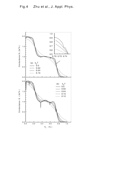
FIG. 4.: The conductance $G$ versus $V_{0}$ at finite temperatures for different SO-interactions: (a) $\alpha^{\prime}=0.005$, with the inset showing an enlargement of the curve around the arrow; (b) $\alpha^{\prime}=0.01$. Other parameters are $E_{f}=1.21$, $\omega_{y}=3\omega_{x}$.

B The effects of magnetic fields

We now discuss the effect of a perpendicular magnetic field on the conductance quantization: the Zeeman effect and the Peierls phase factor. In many theoretical calculations, the Zeeman effect is usually ignored for simplicity. Here we consider both the Peierls phase and the Zeeman effect. Figures.5(a) and (b) show the field-dependent conductance as a function of $V_{0}$ for $\alpha^{\prime}=0,\ 0.01$, respectively. From Fig.5, one of the characteristic features of QPC’s in a magnetic field is that conductance steps begin to appear at odd integer multiples of $G_{0}$ at $\beta\geq 0.09$, due to the lifting of the spin degeneracy by the Zeeman effect. Another feature is that the width of the plateaus is widened when compared to the $\beta=0$ case. On the other hand, the number of effective subbands is decreased when the magnetic field is applied, and actually it is proportional to $1/\beta$.[12] Moreover, figure 5(b) shows that the oscillation as well as the sharp dips are destroyed at high fields. Thus the quality of the quantization is improved when the magnetic field is applied. Certainly, the effect of the SO-interaction is suppressed by a high magnetic field.

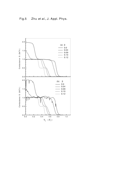
FIG. 5.: The conductance $G$ versus $V_{0}$ in the presence of magnetic field. (a) $\alpha^{\prime}=0,\ k_{B}T=0$; (b) $\alpha^{\prime}=0.01,\ k_{B}T=0$. Other parameters are $E_{f}=1.21$, $\omega_{y}=3\omega_{x}$.

IV Conclusions and discussions

The SO-interaction is equivalent to a momentum-dependent effective magnetic field.[1, 3, 4] However, comparing with a genuine magnetic field, there exist some essential differences in the energy spectra of electrons induced by an effective field or a genuine field, [7] which induce several significant different effects on the conductance. Firstly, spin split energy $\Delta$ induced by the SO-interaction at $|k_{i}=0|$ is zero, while the spectrum induced by a genuine field is determined by the nonzero Zeeman energy $g\mu B_{z}$. This is the reason why the conductance steps do not appear at odd integer multiples of $G_{0}$ in the presence of SO-interaction but zero magnetic field, noting the appearance of this kind of quantized plateaus is the essential feature induced by a genuine field. Secondly, in the presence of SO coupling, there exist bumps ( a nonmonotonic portion) in the spectrum as a function of transverse momentum, while the spectrum is a monotonous function of the momentum in the presence of a genuine magnetic field. Therefore, the reflections at the scattering region in the presence of SO coupling may induce by the negative velocity for $k>0$.[12] It provides us another understanding of the transmission oscillations. Finally, the SO-interaction can remove the spin degeneracy in the band structure but could not lead to an overall spin polarization.[7] Consequently, the $0.7$ structure is unlikely induced by the SO-interaction. On the other hand, the results addressed in the presence of magnetic field may be restricted within weak field since the non-interacting electron model used in the recursive Green’s function is invalid in a very strong magnetic field.

We are now concerned with the possible experimental test of the above SO-induced properties. In unit of $t$, $\alpha^{\prime}=m^{*}\alpha a/\hbar^{2}$, which is estimated to be $(0.54\sim 5.4)\times 10^{-3}$ for some typical semiconductors [ here we choose the parameters of InAs, where $a\sim 0.608\ nm$, $\alpha\sim(1.0\sim 10.0)\times 10^{-10}\ ev\ cm$, and $m^{*}\sim 0.067\ m_{e}$ with $m_{e}$ as the mass of a free electron. [10]]. Thus the oscillations induced by SO coupling may be experimentally observable, depending crucially on the value of $\alpha^{\prime}$.

Finally, we wish to make a few remarks on why the SO-induced effects on the quantized conductance have not been observed in experiments so far. Firstly, the experimental observation on the SO-induced phenomenon would crucially depend on the value of $\alpha^{\prime}$, but $\alpha^{\prime}$ in some typical semiconductor systems may be relatively small based on the above estimation. Thus it is helpful to increase the coupling coefficient in experiments. As indicated by Heida et al., [10] two methods may be used to increase the coefficient $\alpha$ in mesoscopic experiments: one is to increase the electron density $n_{s}$ in QPC since $\alpha$ is proportional to $n_{s}$; and the other is to vary the gate bias which controls the magnitude of the SO-interaction. On the other hand, a larger effective mass of charge carriers would also be helpful for observing the SO-induced oscillations in experiments. Secondly, the SO coupling in the leads has been neglected in the present study. This approximation may enhance the oscillations observed above although the Rashba SO coupling in QPC is larger than that in the leads.[26] It is extremely difficult to include the SO coupling in the leads using the present method because the analytical wave function in the leads should be given; while it appears to be unsolvable in the leads with the SO coupling . Nevertheless, with the advancement of nanotechnology, it is possible to fabricate a mesoscopic structure where the SO coupling is important only in the QPC (i.e., negligible in the two leads). In such systems, it could be easier to observe the SO-induced effects predicted here.

In conclusion, we have generalized a recursive Green’s function approach to calculate numerically the spin-dependent conductance in mesoscopic structures in the presence of SO-interaction and magnetic field. The effect of SO-interaction on the conductance of a QPC is studied in detail. Some interesting oscillations in conductance induced by the SO-interaction have been observed numerically, which may be tested by future mesoscopic experiments.

A

In the appendix we present the recursive Green’s function approach to calculate the spin-dependent transmission $t_{lj}^{\sigma\sigma^{\prime}}$. The electron wave functions in the strip $n$ of the leads can be expressed as a linear combination of eigenfunctions of a straight infinite lead at a given energy $E$. If the incident electron from the left lead is in the $(l,\sigma)$ channel with $l$ and $\sigma$ as the subband and spin indices, the scattering states are represented as

$$| n)_{left}=e^{ik_{l}n}\phi_{k_{l}\sigma}+\sum\limits_{j\sigma^{\prime}}r_{lj}^{\sigma\sigma^{\prime}}e^{-ik_{j}n}\phi_{k_{j}\sigma^{\prime}},$$ (A1)

$$| n)_{right}=\sum\limits_{j\sigma^{\prime}}t_{lj}^{\sigma\sigma^{\prime}}e^{ik_{j}n}\phi_{k_{j}\sigma^{\prime}},$$ (A2)

where $t_{lj}^{\sigma,\sigma^{\prime}}$ ($r_{lj}^{\sigma,\sigma^{\prime}}$) is the transmission (reflection) amplitudes for the incident channel $(l,\sigma)$ and out-going channel $(j,\sigma^{\prime})$, and the wave functions $\phi_{k_{j}\sigma}$ are given by $\phi_{k_{j}\sigma}=\phi_{k_{j}}\otimes\chi(\sigma_{z})$ with

$$\phi_{k_{j}}=\sqrt{\frac{2}{M+1}}(sin\frac{\pi j}{M+1},\cdots,sin\frac{\pi jm}{M+1},\cdots,sin\frac{\pi jM}{M+1})^{T_{r}},$$

and

$$\chi(+)=\left(\begin{array}[]{l}1\\ 0\end{array}\right),\ \ \chi(-)=\left(\begin{array}[]{l}0\\ 1\end{array}\right).$$

Here the sign $T_{r}$ denotes the transposition of matrix. The number of open channels and the value of $k_{j}$ are determined by the Fermi energy from the energy dispersion in ideal leads

$$E=4t-2t(cosk_{j}+cos\frac{\pi j}{M+1}).$$

Only if $k_{j}$ is real do we have a propagating state; we have an evanescent state when $k_{j}$ is imaginary. All real $k_{j}$’s are positive, because we have already considered separately the states propagating to the right (incident and transmitted wave) or to the left (reflected wave). Following the recursive Green’s function technique, we find

$$t_{lj}^{\sigma\sigma^{\prime}}=\sqrt{v_{j}/v_{l}}\phi^{+}_{k_{j}\sigma^{\prime}}G_{N+1,0}\Theta(\sigma)\phi_{k_{l}\sigma}e^{-ik_{j}L_{x}},$$ (A3)

where

$$v_{j}=\frac{1}{\hbar}\frac{\partial E}{\partial k_{j}},$$

$$\Theta(\sigma)=-2it\sum\limits_{l=1}^{M}sink_{l}[Q_{l}\otimes\zeta(\sigma_{z})],$$

with

$$(Q_{l})_{pp^{\prime}}=\frac{2}{M+1}sin\frac{l\pi p}{M+1}sin\frac{l\pi p^{\prime}}{M+1},\ (p,p^{\prime}=1,\cdots,M),$$

$$\zeta(+)=\left(\begin{array}[]{lc}1&0\\ 0&0\end{array}\right),\ \ \zeta(-)=\left(\begin{array}[]{lc}0&0\\ 0&1\end{array}\right).$$

The set of vectors $\phi^{+}_{k_{j}\sigma^{\prime}}$ are the duals of the set $\phi_{k_{l}\sigma}$, defined by $\phi^{+}_{k_{j}\sigma^{\prime}}\phi_{k_{l}\sigma}=\delta_{jl}\delta_{\sigma^{\prime}\sigma}$. $G_{N+1,0}$ is the retarded Green’s function for the scattering region between two ideal leads, which can be obtained by a set of recursion formulas in a matrix form, [24]

$$G_{n^{\prime}+1,0} = g^{n^{\prime}+1}H_{n^{\prime}+1,n^{\prime}}G_{n^{\prime},0},\ \ (0\leq n^{\prime}\leq N)$$ (A4)

$$g^{n^{\prime}+1} = [E-\widetilde{H}_{n^{\prime}+1}-\Lambda^{n^{\prime}}]^{-1},$$ (A5)

$$(\Lambda^{n^{\prime}})_{pp^{\prime}} = e^{i2\pi(p-p^{\prime})\beta}V_{x}^{+}(g^{n^{\prime}})_{pp^{\prime}}V_{x},\ \ (p,p^{\prime}=1,\cdots,M)$$ (A6)

by iteration starting form $g^{0}=G_{0,0}=(E-\widetilde{H}_{0})^{-1}$, where $\widetilde{H}_{0}=H_{0}-tF(\sigma_{in})$, $\widetilde{H}_{l}=H_{l}\ (1\leq l\leq N)$, $\widetilde{H}_{N+1}=H_{N+1}-tF(\sigma_{out})$ with $\sigma_{in}$ $(\sigma_{out})$ as the spin state of the incident (outgoing) electrons, and

$$F(\sigma)=\sum\limits_{j=1}^{M}e^{ik_{j}}[Q_{j}\otimes\zeta(\sigma_{z})],$$ (A7)

It is worth pointing out that each element of Green’s function in the above recursion formula is given by a quaternion number in the presence of the SO-interaction or the Zeeman effect.[25] In the numerical calculations of $G_{N+1,0}$ and $\Theta(\sigma)$ in Eq.(A3), we have used explicitly the multiplication table for quaternion number.

REFERENCES

- [1] Y. Meir, Y. Gefen, and O. Entin-Wohlman, Phys. Rev. Lett. 63, 798 (1989).
- [2] D. Loss and P. M. Goldbart, Phys. Rev. B 45, 13 544 (1992).
- [3] A. G. Aronov and Y. B. Lyanda-Geller, Phys. Rev. Lett. 70, 343 (1993).
- [4] Y. C. Zhou, H. Z. Li, and X. Xue, Phys. Rev. B 49, 14 010 (1994); S. L. Zhu, Y. C. Zhou, and H. Z. Li, ibid. 52, 7814 (1995). Z. D. Wang and S. L. Zhu, ibid. 60, 10 668 (1999).
- [5] S. L. Zhu and Z. D. Wang, Phys. Rev. Lett. 85, 1076 (2000); S. L. Zhu, Z. D. Wang, and Y. D. Zhang, Phys. Rev. B 61, 1142 (2000).
- [6] A. F. Morpurgo, J. P. Heida, T. M. Klapwijk, B. J. van Wees, and G. Borghs, Phys. Rev. Lett. 80, 1050 (1998).
- [7] A. V. Moroz and C. H. W. Barnes, Phys. Rev. B 60, 14 272 (1999); ibid. 61, R2464 (2000).
- [8] E. N. Bulgakov, K. N. Pichugin, A. F. Sadreev, P. Str̆eda, and P. S̆eba, Phys. Rev. Lett. 83, 376 (1999).
- [9] In a system of two-dimensional electron gas (2DEG) in the absence of external magnetic field, the spin of a moving electron feels an effective magnetic field induced by a perpendicular interface electric field. This kind of SO-interaction is commonly referred to as the Rashba SO-interaction. See E. I. Rashba, Sov. Phys. Solid State 2, 1109 (1960).
- [10] J. Luo, H. Munekata, F. F. Fang, and P. J. Stiles, Phys. Rev. B 38, 10 142 (1988); J. Nitta, T. Akazaki, H. Takayanagi, and T. Enoki, Phys. Rev. Lett. 78, 1335 (1997); J. P. Heida, B. J. van Wees, J. J. Kuipers, T. M. Klapwijk, and G. Borghs, Phys. Rev. B 57, 11 911 (1998).
- [11] G. Lommer, F. Malcher, and U. Rössler, Phys. Rev. Lett. 60, 728 (1988).
- [12] B. J. van Wees, H. van Houten, C. W. Beenakker, J. G. Williamson, L. P. Kouwenhoven, D. van der Marel, and C. T. Foxon. Phys. Rev. Lett. 60, 848 (1988); B. J. van Wees, L. P. Kouwenhoven, E. M. M. Willems, C. J. P. M. Harmans, J. E. Mooij, H. van Houten, C. W. J. Beenakker, J. G. Williamson, and C. T. Foxon, Phys. Rev. B 43, 12 431 (1991).
- [13] D. A. Wharam, T. J. Thornton, R. Newbury, M. Pepper, H. Ahmed, J. E. F. Frost, D. G. Hasko, D. C. Peacock, D. A. Ritchie, and G. A. C. Jones, J. Phys. B 21, L209 (1988).
- [14] K. J. Thomas, J. T. Nicholls, M. Y. Simmons, M.Pepper, D. R. Mace, and D. A. Ritchie, Phys. Rev. Lett. 77, 135 (1996).
- [15] T. Ando, Phys. Rev. B 44, 8017 (1991).
- [16] S. Sanvito, C. J. Lambert, J. H. Jefferson, and A. M. Bratkovsky, Phys. Rev. B 59, 11 936 (1999).
- [17] J. C. Cuevas, A. L. Yeyati, and A. Martĺn-Rodero, Phys. Rev. Lett. 80, 1066 (1998); J. C. Cuevas, A. Matĺn-Rodero, and A. L. Yeyati, Phys. Rev. B 54, 7366 (1996).
- [18] S. Datta, Electronic transport in mesoscopic systems (the Press Syndicate of the Cambridge University, New York, 1995), pp145-146.
- [19] P. A. Lee and D. S. Fisher, Phys. Rev. Lett. 47, 882 (1981); A. MacKinnon, Z. Phys. B 59, 385 (1985).
- [20] R. Landauer, IBM J. Res. Dev. 1, 223 (1957); M. Büttiker, Phys. Rev. Lett. 57, 1761 (1986).
- [21] M. Büttiker, Phys. Rev. B 41, 7906 (1990).
- [22] For different system sizes, we observe that the main properties are the same as long as , which implies that the transport properties addressed below are almost independent on the system size.
- [23] Equation (10) is clearly oversimplified since is assumed to be the reflection probability on the interfaces between the ideal leads and the scattering region, we can nevertheless apply it to understand some features of the transmission oscillations, as done by van Wess et al in explaining the oscillations observed in their experimental data.[12]
- [24] The results in spin-independent cases can be found in Refs.[15, 19].
- [25] Each element in the above Green’s function is a complex number if only the Peierls phase factor associated with the magnetic field is considered (both the Zeeman effect and the SO coupling are ignored).
- [26] The QPC is often produced by a negative gate while the negative gate enhances the Rashba SO coupling. This effect was verified experimentally by Nitta et al in Ref.[10].