Study on the Kondo effect in the tunneling phenomena through a quantum dot

Abstract

We review our recent studies on the Kondo effect in the tunneling phenomena through quantum dot systems. Numerical methods to calculate reliable tunneling conductance are developed. In the first place, a case in which electrons of odd number occupy the dot is studied, and experimental results are analyzed based on the calculated result. Tunneling anomaly in the even-number-electron occupation case, which is recently observed in experiment and is ascribed to the Kondo effect in the spin singlet-triplet cross over transition region, is also examined theoretically.

,

1 Introduction

Quantum dot systems are now designed as the artificial magnetic impurity and are growing as a field of detailed experimental studies of the Kondo problems[1] . In this report we review our recent theoretical works on the Kondo effect in the tunneling phenomena through quantum dot[2, 3, 4].

After the papers pointed out the possibility to occur the Kondo effect in tunneling through a quantum dot[5], many theoretical studies have been done on this problem[6]. The calculation of the tunneling conductance needs the dynamical excitation spectra. However we have not exact analytic calculation of the dynamical excitation spectra for the Kondo systems[7]. Two numerical methods have been recently developed to calculate the tunneling conductance of the quantum dot systems. One is based on the numerical renormalization group technique (NRG)[8], and another is based on the Quantum Monte Carlo (QMC) technique[3]. Both techniques are known as reliable methods to calculate the dynamical excitation of the Kondo systems[7, 9, 10].

When the occupation number of electrons on the dot is odd, localized spin freedom appears on the dot, and it couples with the conduction electrons on the leads. At very low temperatures, we can expect the increase of the tunneling conductance due to the resonance transmission via the Kondo peak in the density of states on the dot orbitals. This is the most typical example of the Kondo effect of the dot systems, and has been observed in many experiments[1]. In the first part of this report, we present the theoretical calculation for this case[2] and compare it with experimental data[11]. Recently, anomaly in a region of an even electron number occupation case has been reported in experiment[12]. This phenomena is expected to relate to the Kondo effect in the spin crossover region of even occupation number case[4, 13, 14]. This problem is discussed in the second part of this report.

2 Single Orbital Case

We consider the following Hamiltonian,

$$H = H_{\rm\ell}+H_{\rm d}+H_{\rm\ell-d},$$ (1)

$$H_{\rm\ell} = \sum_{\mu k\sigma}\varepsilon_{\mu k}c_{\mu k\sigma}^{+}c_{\mu k\sigma},$$ (2)

$$H_{\rm d} = \sum_{p\sigma}\varepsilon_{dp}n_{dp\sigma}+U\sum_{<p\sigma,p^{\prime}\sigma>}n_{dp\sigma}n_{dp^{\prime}\sigma^{\prime}},$$ (3)

$$H_{\rm\ell-d} = \frac{1}{\sqrt{N}}\sum_{p\mu k\sigma}\{v_{p\mu k}d_{p\sigma}^{+}c_{\mu k\sigma}+{\rm h.c.}\}.$$ (4)

The terms $H_{\rm\ell}$ and $H_{\rm d}$ represent the electron in the leads and the dot, respectively. The term $H_{\rm\ell-d}$ gives the electron tunneling between the leads and the dot. The suffix $\mu=L(R)$ means the left(right) lead and $dp$ means the dot orbital denoted by $p$. The quantity $\varepsilon_{dp}$ corresponds to the energy of the orbital, and it can be changed by applying gate voltage. The quantity $U$ is the Coulomb interaction constant.

At first we consider the most simplified model that the dot has a single orbital. We abbreviate the suffix $p$. There will be many orbitals in dot in actual situations. Two orbitals case will be discussed in §3. We calculate the conductance, $G$, in the linear theory of the bias voltage. It is obtained from the correlation function of the current operators[8]. But in the single orbital case, the calculation is reduced to the following expression[3],

$$G=\frac{2e^{2}}{h}\int\frac{4\Gamma_{L}\Gamma_{R}}{\Gamma_{L}+\Gamma_{R}}(-{\rm Im}G_{dd}(\epsilon))\bigl{(}-\frac{\partial f}{\partial\epsilon}\bigr{)}{\rm d}\epsilon,$$ (5)

where $G_{dd}(\epsilon)$ is Green’s function of the dot orbital and $f(\epsilon)$ is the Fermi distribution function. We use this formula in this section because the numerical calculation of $G_{dd}(\epsilon)$ is easier than the calculation of the current correlation function. Detailed comparison of both methods are made in Ref.[3]. Hereafter we assume that the leads have constant density of states from $-D$ to $D$ with $D=1$. The hybridization strength is parameterized as $\Gamma_{\mu}=\pi|v_{\mu}|^{2}\rho_{c}$, where $\rho_{c}=1/2D$ is the density of states for the lead.

In Fig.1, we show the conductance as a function of the gate voltage ($\varepsilon_{d}$) for various temperature cases[2]. This calculation is carried out by the NRG method. At higher temperatures we have paired Coulomb oscillation peaks at $\varepsilon_{d}=-U$ and 0. They grow without increase of their width, thus become very sharp as the temperature decreases. At the same time the peak positions shift slightly to $\varepsilon_{d}=-U/2$ side. When the temperature decreases further, the intensity of the valley region between the two peaks gradually increases, and the peaks merge into a broad single peak at extremely low temperature. The characteristic temperature $T_{\rm KM}$ varies drastically as $\varepsilon_{d}$ changes. (We define $T_{\rm KM}$ following the usual definition, $T_{\rm K}=4\chi(T=0)$, for each $\varepsilon_{d}$ case). It is the lowest at the mid point of the two peaks, $\varepsilon_{d}=-U/2$, and is denoted as $T_{\rm KM}^{*}$, which is $T_{\rm KM}^{*}/U=5.34\times 10^{-7}$ for the parameter case used in Fig.1. The conductance at the mid point begin to increase at about $10T_{\rm KM}^{*}$, and the valley disappears at about $0.2T_{\rm KM}^{*}$.

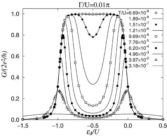
Figure 1: Conductance as a function of $\varepsilon_{d}$ for the parameter $\Gamma/(\pi U)=1.0\times 10^{-2}$ ($U=1.0\times 10^{-2},\Gamma/\pi=1.0\times 10^{-4}$).

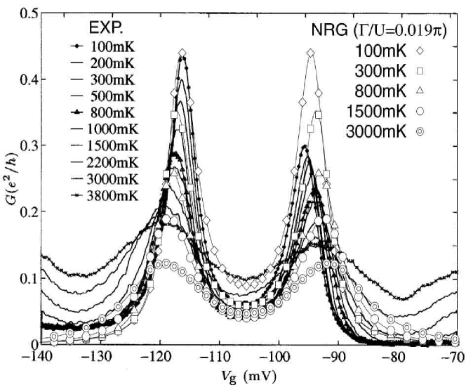
Figure 2: Comparison between the experimental and the calculated data. The experimental data is reproduced from Fig.2 of Ref.[11]. The parameter of the NRG calculation is chosen to be $\Gamma/(\pi U)=1.9\times 10^{-2}$

Goldhaber-Gordon et al. have shown the detailed temperature dependence of the conductance[11]. We directly compare the NRG data with experimental data in Fig.2[2]. The Coulomb repulsion has been estimated to be 1.9 meV. We have estimated $\Gamma=0.12$meV =($1.3\times 10^{3}$mK), and thus $\Gamma/\pi U=1.9\times 10^{-2}$ in the experimental situation. On horizontal axis the points $\varepsilon_{d}=0,-U$ of the calculated conductance are set at $V_{g}=-119,-92$meV, respectively, and factor 0.31 is multiplied to the NRG data to fit the experimental data at the lowest temperature. This factor 0.31 would be caused by the asymmetry $\Gamma_{\rm L}\neq\Gamma_{\rm R}$. For the left hand side peak, the conductance data agrees very well with the experimental one in 100 mK $\sim$ T $\sim$ 1500mK. This agreement suggests that the behaviors in experiment are caused by the Kondo effect in the mid-temperature region shown in Fig.1. The Kondo temperature at the valley region seems to be less than 10 mK.

There are several discrepant points. At high temperature region T $\geq$ 2000mK, the conductance of the experimental data is larger than that of the NRG data. This might be caused by the multi-orbital effect. The conductance shows disagreement in the valley and the right hand peak positions. The change of the gate voltage on the dot will affect not only the potential of the dot, but also the hybridization strength between the dot and the lead states.

The conductance at low temperature is strongly suppressed by application of the Zeeman field. The theoretical study has been carried out based on the QMC method[3], and the result agrees well with experimental one[15].

3 Spin Crossover Transition

Recently, Sasaki et al. observed low temperature tunneling anomaly in even-number-electron-occupation case[12]. They controlled the energy splitting of orbitals by tuning the magnetic field[16]. When the level splitting is gradually increased in the even electron number case, the energy of the spin triplet state increases compared with that of the singlet state. The electrons occupy different orbitals to gain Hund’s coupling energy in the former state, while the electrons with opposite spin occupy the lower energy orbital in the latter state. It was suggested that the low temperature anomaly is related to the Kondo effect due to this spin crossover transition[13, 14]. However detailed calculation of the conductance has not been done. It is observed that a bump grows between the two Coulomb peaks, i.e., a third peak appears between the Coulomb peaks and it grows when the temperature decreases. This behavior is quite different from that of the odd number case discussed in previous section.

We calculate the conductance around the singlet-triplet crossover region for a system with two orbitals[4]. The orbitals are denoted as even($p$=e) and odd($p$=o). The energy of e(o) orbital is defined as $\varepsilon_{d}-\delta/2$ ($\varepsilon_{d}+\delta/2$). The exchange term $H_{\rm ex}=J_{\rm H}\sum_{\sigma_{1}\sigma_{2}\sigma_{3}\sigma_{3}}(\mbox{\boldmath$\sigma$})_{\sigma_{1}\sigma_{2}}(\mbox{\boldmath$\sigma$})_{\sigma_{3}\sigma_{4}}d^{+}_{{\rm e}\sigma_{1}}d_{{\rm e}\sigma_{2}}d^{+}_{{\rm o}\sigma_{3}}d_{{\rm o}\sigma_{4}}$ is added to the Hamiltonian Eq.(1). ($J_{\rm H}<0$)

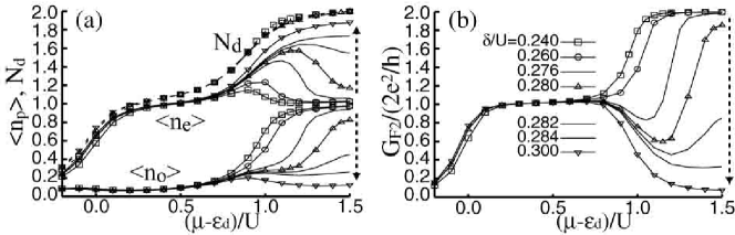
Figure 3: (a) Occupation numbers of the e and o orbitals at $T=0$, $\langle n_{\rm e}\rangle$, $\langle n_{\rm o}\rangle$, and the total occupation number on the dot, $N_{\rm d}$. (b) Conductance at $T=0$ for the two channel case, $G_{F2}$. The symbols for $\delta$ are common in (a) and (b). The dashed arrows show the increasing of $\delta$. Parameters are $J_{\rm H}/{U}=-0.3$, $\Gamma_{\rm e}/U=\Gamma_{\rm o}/U=0.02$.

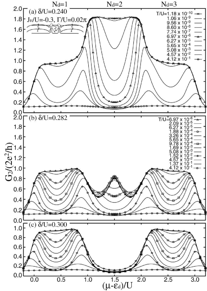
Figure 4: Conductance at various temperatures as a function of gate voltage in the two channel case. (a)$\delta/U=0.24$, (b)$\delta/U=0.282$, (c)$\delta/U=0.3$. The symbols of the temperature in (b) and (c) are common.

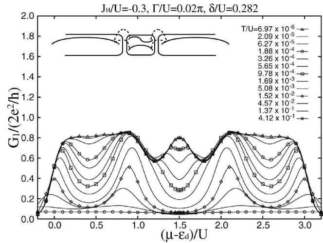
Figure 5: Conductance as a function of gate voltage in the single channel case. Parameters are the same to those of Fig.4(b).

In Fig.3(a), we show the occupation numbers of the even and odd orbitals, $\langle n_{\rm e}\rangle$ and $\langle n_{\rm o}\rangle$, on the dot. The parameters are $J_{\rm H}/U=-0.3$, $\Gamma_{\rm e}/U=\Gamma_{\rm o}/U=0.02\pi$.

We assume the case in which both leads have two conduction channels, and each dot orbital connects to each conduction channel (two channel case). The conductance is given as the sum of ones from two channels. At very low temperatures it is given as, $G_{\rm F2}=(2e^{2}/h)\sum_{p}\sin^{2}(\pi\langle n_{p}\rangle/2)$, and is shown in Fig.3(b).

Here we define a quantity $x=(\mu-\varepsilon_{d})/U$. In the $0\sim x\sim 1$ region, an electron occupies the e-orbital, $(\langle n_{\rm e}\rangle,\langle n_{\rm o}\rangle)\simeq(1,0)$. Next we see the $1\sim x\sim 1.5$ region. At $\delta/U=0.24$, the occupations on both orbitals are almost the same, $(\langle n_{\rm e}\rangle,\langle n_{\rm o}\rangle)\simeq(1,1)$, due to the strong Hund’s coupling. When $\delta$ increases, the occupations in the $1\sim x\sim 1.5$ region gradually split to $(2,0)$ where the local spin state is a singlet. Therefore the conductance decreases from $4e^{2}/h$ to $0$. We stress that the splitting is suppressed around $x=1.5$ as seen in Fig.3(a). For example at $\delta/U=0.28$, the second electron tends to occupy the e-orbital when $x$ sweeps to $x=1.2$ from smaller $x$, then they redistribute to the e- and o-orbitals when $x$ further sweeps to $x=1.5$; $(1,0)\rightarrow(1.6,0.3)\rightarrow(1.2,0.8)$. This redistribution reflects the stronger Hund’s coupling near $x=1.5$, at which the total occupation is close to two. The redistribution causes a bump in the conductance around $x=1.5$ at low temperatures, as seen in $0.276\sim\delta/U\sim 0.284$ in Fig.3(b).

In Fig.4 we show the conductance at various temperatures around the local spin singlet-triplet degeneracy. The parameters are: (a) $\delta/U=0.24$, (b), $\delta/U=0.282$, (c) $\delta/U=0.3$. There are the four Coulomb peaks on $x=(\mu-\varepsilon_{\rm d})/U\sim 0$, $1$, $2$, $3$ at high temperatures. When the temperature decreases, the conductance in the region $0\sim x\sim 1$ ($2\sim x\sim 3$), where $N_{\rm d}\simeq 1$ ($N_{\rm d}\simeq 3$), increases to $\simeq 2e^{2}/h$, caused by the usual spin-1/2 Kondo effect for the e-channel (o-channel). On the other hand, the region $1\sim x\sim 2$, where $N_{\rm d}\simeq 2$, is remarkable. At (a) $\delta/U=0.24$, the conductance is large, about $4e^{2}/h$. However, the large conductance appears at extremely low temperature (e.g., $T/U=10^{-8}$ corresponds to $10^{-3}{\rm mK}$ for $U\simeq{\rm 10meV}$). When $\delta$ increases to (b) $\delta/U=0.282$, a ”bump” emerges in the region $1.2\sim x\sim 1.8$ as the temperature decreases. For the case (c) $\delta/U=0.3$, the conductance in the region $1\sim x\sim 2$ is nearly constant with a small value. The behaviors (a)-(c) are classified into, (a) the local spin triplet Kondo effect, (b) the singlet-triplet Kondo effect, and (c) the usual even-odd oscillations for the dot with large energy separation [1, 8].

Next we consider a case in which leads have only one conduction channel, and the both dot orbitals connect to this single channel (single channel case). In such case one orbital will hybridize mainly with even combination of L and R lead states, and another mainly with odd combination of L and R states. The tunneling via different orbitals interferes in this case. At $T=0$, the conductance is given as $G_{\rm F1}=(2e^{2}/h)\sin^{2}(\pi(\langle n_{e}\rangle-\langle n_{o}\rangle)/2)$ , and is small when $\langle n_{e}\rangle\simeq\langle n_{o}\rangle$. Therefore the conductance will tend to zero as $T$ decreases to extreme low temperature when Hund’s rule coupling energy dominates. This is contrasted to the case (a) in Fig.4.

In the singlet-triplet Kondo effect case where the Kondo temperature is not low, the calculated temperature dependence of the conductance is not so different from that of the two channel case(Fig.4(b)) as seen from Fig.5. This is because $\langle n_{e}\rangle$ and $\langle n_{o}\rangle$ have different and not-integer values as seen from Fig.3(a).

As a summary, we have shown that the electron occupation on orbitals redistribute to gain Hund’s coupling energy in the singlet-triplet crossover region when the potential deepens. This redistribution causes a bump, as seen in the experiment, in the conductance at low temperatures.

References

- [1] D. Goldhaber-Gordon et al., Nature 391 (1998) 156, S. M. Cronenwett et al., Science 281 (1998) 540, W. G. van der Wiel et al., Science 289 (2000) 2105.
- [2] W. Izumida et al., J. Phys. Soc. Jpn. 70 (2001) 1045.
- [3] O. Sakai et al., J. Phys. Soc. Jpn. 68 (1999) 1640.
- [4] W. Izumida et al., Phys. Rev. Lett. 87 (2001) 216803.
- [5] L. I. Glazman et al., JETP Lett. 47 (1988) 452, T. K. Ng et al., Phys. Rev. Lett. 61 (1988) 1768, A. Kawabata J. Phys. Soc. Jpn. 60 (1991) 3222.
- [6] For references see for example Ref.[2].
- [7] A. C. Hewson, The Kondo problem to Heavy fermions, (Cambridge University Press, Cambridge, 1993)
- [8] W. Izumida et al., J. Phys. Soc. Jpn. 66 (1997) 717, ibid. 67 (1998) 2444.
- [9] O. Sakai et al., J. Phys. Soc. Jpn. 58 (1989) 1690.
- [10] J. E. Gubernatis et al., Phys. Rev. B 44 (1991) 6011.
- [11] D. Goldhaber-Gordon et al., Phys. Rev. Lett. 81 (1998) 5225.
- [12] S. Sasaki et al., Nature (London) 405 (2000) 764.
- [13] M. Eto et al., Phys. Rev. Lett. 85 (2000) 1306.
- [14] M. Pustilnik et al., Phys. Rev. Lett. 85 (2000) 2993.
- [15] L. P. Rokhinson et al., P. Rev. B 60 (1999) R16319.
- [16] We can neglect the Zeeman splitting in this case, see for example [4].