Electronic spin precession in semiconductor quantum dots with spin-orbit coupling

Abstract

The electronic spin precession in semiconductor dots is strongly affected by the spin-orbit coupling. We present a theory of the electronic spin resonance at low magnetic fields that predicts a strong dependence on the dot occupation, the magnetic field and the spin-orbit coupling strength. Coulomb interaction effects are also taken into account in a numerical approach.

In recent years the spin properties of non-magnetic semiconductors have attracted an increasing attention, not only for the fundamental physics behind the subject but also for the future technological applications of the electronic spin in spin-based devices [1]. The available experimental techniques allow for a precise observation of spin dynamics in a wide range of semiconductor structures. Actually, spin precession can be monitored with femtosecond resolution using time resolved Faraday rotation, as reported in Ref. [2] for GaAs quantum wells; and in Ref. [3] for CdSe excitonic quantum dots. Another exciting possibility comes from spatially resolved spin detection, achieved in Ref. [4] for organic molecules on a graphitic surface by combining the spatial resolution of scanning-tunneling microscopy (STM) with the spin sensitivity of electron-spin resonance (ESR).

In this work we report a theoretical study of the spin precessional properties of electrons confined to a model GaAs quantum dot, including spin-orbit (SO) coupling. This mechanism gives rise to a rich variety of spin precessional frequencies, depending on the orbital state of the electrons, even in the absence of a vertical magnetic field; as compared to the Larmor frequency for systems without SO coupling.

In order to model a GaAs quantum dot with SO coupling for the standard (001) plane [5], we add to the Hamiltonian the Dresselhaus term originating from the bulk inversion asymmetry:

$${\cal H}_{D}=\frac{\lambda_{D}}{\hbar}\sum_{i=1}^{N}{\left[\,P_{x}\sigma_{x}-P_{y}\sigma_{y}\,\right]_{i}}\;,$$ (1)

where the $\sigma$’s are the Pauli matrices and ${\bf P}=-i\hbar\nabla+\frac{e}{c}{\bf A}$ represents the canonical momentum containing the vector potential ${\bf A}$ —within the symmetric gauge for a vertical magnetic field $B$ one has ${\bf A}=\frac{B}{2}(-y,x)$. The intensity of the SO term depends on the effective dot height $z_{0}$ as [6] $\lambda_{D}\approx\gamma(\pi/z_{0})^{2}$ where $\gamma$ is a material dependent constant that for GaAs takes the value $\gamma=27.5$ eVų [7]. In the present work we shall consider $\lambda_{D}$ parameters in the range $[\,0.44\,,\,1.08\,]\times 10^{-9}\;{\rm eV}{\rm cm}$, in the same order of magnitude of those found in the literature for GaAs/AlGaAs heterojunctions [8] ($0.25\times 10^{-9}\;{\rm eV}{\rm cm}$ for electrons, $0.6\times 10^{-9}\;{\rm eV}{\rm cm}$ for holes).

In the following, the dot vertical extent only determines the SO coupling strength, the electronic motion is otherwise considered bidimensional in a lateral confinement potential with circular symmetry, $V(r)$. Taking into account the Zeeman ${\cal H}_{Z}$ and spatial ${\cal H}_{0}$ energies and neglecting for the moment electron-electron interaction, the full Hamiltonian reads ${\cal H}={\cal H}_{0}+{\cal H}_{D}+{\cal H}_{Z}$, where

$${\cal H}_{0} = \sum_{i=1}^{N}{\left[\rule{0.0pt}{14.22636pt}\right.\frac{{\bf P}^{2}}{2m^{*}}+V(r)\left.\rule{0.0pt}{14.22636pt}\right]_{i}}\;,$$ (2)

$${\cal H}_{Z} = \sum_{i=1}^{N}{\left[\rule{0.0pt}{14.22636pt}\right.\frac{1}{2}g^{*}\mu_{B}B\sigma_{z}\left.\rule{0.0pt}{14.22636pt}\right]_{i}}\;.$$ (3)

In Eqs. (2) and (3) $\mu_{B}$ denotes the Bohr magneton while $m^{*}$ and $g^{*}$ are, respectively, the effective mass and gyromagnetic factor for the conduction band of bulk GaAs, i.e., $m^{*}=0.067\,m_{e}$ and $g^{*}=-0.44$.

For ${\cal H}_{0}\gg{\cal H}_{D}\gg{\cal H}_{Z}$ a diagonalization in spin space to order $\lambda_{D}^{2}$ can be obtained by means of a unitary transformation [9] to a new Hamiltonian $\tilde{\cal H}=U^{+}{\cal H}U$, with

$$\tilde{\cal H} = \sum_{i=1}^{N}{\left[\rule{0.0pt}{14.22636pt}\right.{{\bf P}^{2}\over 2m^{*}}+V(r)}+\lambda_{D}^{2}\frac{m^{*}}{\hbar^{3}}\,(xP_{y}-yP_{x})\sigma_{z}$$ (4)

$$+ \frac{1}{2}\,g^{*}\mu_{B}B\sigma_{z}\left.\rule{0.0pt}{14.22636pt}\right]_{i}-N\lambda_{D}^{2}\frac{m^{*}}{\hbar^{2}}+O(\lambda_{D}^{3})\;.$$ (5)

In the new, intrinsic, reference frame the eigenstates are orbitals with well defined spin and spatial angular momentum in $z$ direction, i.e., $\varphi_{n\ell\pm}({\bf r})\chi_{\pm}(\eta)$; where $\eta=\uparrow,\downarrow$ and $\sigma_{z}\chi_{\pm}=\pm\chi_{\pm}$. Note that the spatial parts also depend on the spin label since the effective radial confinement in Eq. (4) is different for $\chi_{+}$ and $\chi_{-}$ orbitals. When these eigenstates are transformed back to the laboratory frame, spin and angular momentum become ill defined, but they deviate little from the well defined intrinsic values. Therefore, we shall retain the intrinsic labels $(n\ell\pm)$ to characterize the laboratory-frame eigenstates

$$\chi_{n\ell+}({\bf r},\eta) \equiv \varphi_{n\ell+}({\bf r}){1\choose-i\lambda_{D}\frac{m^{*}}{\hbar^{2}}re^{-i\phi}}$$ (6)

$$\chi_{n\ell-}({\bf r},\eta) \equiv \varphi_{n\ell-}({\bf r}){-i\lambda_{D}\frac{m^{*}}{\hbar^{2}}re^{i\phi}\choose 1}\;.$$ (7)

Using this approach, in Ref. [10] we showed that the static spin of odd-$N$ quantum dots alternates between up and down states as a consequence of the SO coupling when the magnetic field and/or the SO coupling strength are varied. Other static properties have been studied by Governale [11] using a SO coupling of the Rashba type, unitarily equivalent to the Dresselhaus contribution [9]. Here we shall focus on the dynamical spin evolution in a model quantum dot when all the system parameters are kept fixed.

In order to excite the electronic spin precession one needs to perturb the ground state spin configuration. The usual way to achieve this consists in applying a horizontal magnetic field for a certain time interval that rotates the spin and triggers the precessional motion. By performing a spin rotation about an arbitrary horizontal axis of the above given spinors and decomposing the result in the stationary basis (6), we observe some interesting features. In absence of SO coupling ($\lambda_{D}=0$) the only allowed transitions are the spin flips $(n\ell+)\leftrightarrow(n\ell-)$, leading to an in-plane spin precession at the usual Larmor frequency $\omega_{L}=|g^{*}|\mu_{B}B/\hbar$. This is a well-known result valid even when spin-independent interactions are present [12]. When SO coupling is considered, besides the pure spin flips other transitions involving additional changes in $\ell$ and/or $n$ are allowed. In addition to monopolar $\delta\ell=0$, dipolar $\delta\ell=\pm 1$ and quadrupolar $\delta\ell=2$ spin flip transitions also contribute with different weights. As we shall show below the $\delta\ell=0$ transitions of the pure Larmor mode are still the dominant ones in the precessional spectrum with SO coupling; the dipolar ones are weaker by more than an order of magnitude while the quadrupolar spin flip excitations turn out to be negligible in all cases studied. It is worth to point out that even transitions between orbitals with different $n$ could contribute because of the non orthogonality of $+$ and $-$ radial functions, although these will normally involve high energies and low strengths due to the small deviation from pure orthogonality.

To quantify the SO coupling effect we shall assume a parabolic confinement potential whose eigenenergies and eigenstates are analytically known:[13].

$$V({\bf r})=\frac{1}{2}m^{*}\omega_{0}^{2}(x^{2}+y^{2})\;.$$ (8)

With the above analysis the lowest $\delta\ell=0$ spin-flip mode, that we shall call the SO precessional mode $\omega_{\cal P}$, has a frequency, in the low $\lambda_{D}$ limit,

$$\omega_{\cal P}=\left|\rule{0.0pt}{21.33955pt}\right.\omega_{L} + 2\,\ell\,\lambda_{D}^{2}\frac{m^{*}}{\hbar^{4}}$$ (9)

$$- (2n+|\ell|+1){\lambda_{D}^{2}\omega_{c}\over\sqrt{\omega_{0}^{2}+\frac{\omega_{c}^{2}}{4}}}\frac{m^{*}}{\hbar^{4}}\left.\rule{0.0pt}{21.33955pt}\right|\;.$$ (10)

The SO precessional mode $\omega_{\cal P}$ is the dominant excitation in the spin rotation spectrum and it can be considered in a natural way as the modification of the pure Larmor mode $\omega_{L}$ by the SO coupling. Note that in Eq. (9) we have introduced the usual cyclotron frequency $\omega_{c}=eB/(m^{*}c)$ and that $\ell$ is the angular momentum in the intrinsic frame of the precessionally active orbital, i.e., that with spin flips allowed by the Pauli principle; normally the highest or the second highest occupied level in an odd-$N$ dot. Even $N$ systems will generally not possess a net spin at low enough magnetic fields ${\cal H}_{D}\gg{\cal H}_{Z}$.

Equation (9) already allows us to point out several interesting predictions: a) At $B=0$ the SO precessional frequency does not vanish when $\ell\neq 0$, with the offset indicating the SO coupling intensity. b) In general, positive and negative $\ell$ orbitals will display different $B$ dispersions for a fixed $\lambda_{D}$. c) When the precessionally active orbital changes due to an internal rearrangement the SO precessional frequency will display a discontinuity.

It is worth to mention that a $B=0$ offset similar to the one mentioned above was observed in GaAs quantum wells already in 1983 [14] and that a zero-field level splitting in quantum dots was also discussed in Ref. [6]. Note that since the SO coupling term is time reversal invariant Kramers degeneracy is preserved at $B=0$ and, therefore, the precessional offset can be found only when the transition involves non-conjugate states.

The validity of the preceding $O(\lambda_{D}^{2})$ analysis can be tested with direct numerical calculations which avoid the approximate diagonalization procedure. To this end, we have implemented in a spatial grid the solution to the time-dependent Schrödinger equation, labelling the discrete set of orbitals by an index $j$,

$$i\hbar\frac{\partial}{\partial t}\chi_{j}({\bf r},\eta)=\sum_{\eta^{\prime}}{h_{sp}({\bf r},\eta\eta^{\prime})\;\chi_{j}({\bf r},\eta^{\prime})}\;;$$ (11)

where we have defined the single-particle Hamiltonian from

$${\cal H}\equiv\sum_{i=1}^{N}{h_{sp}({\bf r}_{i},\eta_{i}\eta^{\prime}_{i}})\;.$$ (12)

A ‘real time’ simulation of the precession can be performed by taking the stationary solutions to Eq. (11), rotate in spin space with a given horizontal axis (say the $x$ axis) and use the resulting perturbed spinors as starting point for the time evolution. Figure 1 displays one such simulation for a $N=7$ quantum dot. The analysis is based on the $x$-component of the total spin, in time (lower panel) and energy (upper panel) domains. The different features discussed above in the analytical model are nicely manifested by the numerical signals. From Fig. 1 we can also see quantitatively the strength of the SO precessional mode with respect to the doubly split upper and lower branches of the dipole modes. The minor energy differences between the numerical and analytical peak positions can be attributed to effects beyond $O(\lambda_{D}^{2})$ and, also, to a slight departure from the ${\cal H}_{Z}\ll{\cal H}_{D}$ limit for a finite $B$.

A shortcoming of the time simulation technique is found in the determination of very low energy excitations. Low frequency signals may require extremely long simulation times, exceeding the limit of computational feasibility; either by excessive computing time or by accumulated numerical error. In our case, we have estimated this limit at $T_{\em max}\approx 100\,{\rm ps}$ and the corresponding minimum frequency $\omega_{\em min}/2\pi\approx 10\,{\rm GHz}$. Nevertheless, in the noninteracting case one can directly compute the perturbative strength function from the stationary ground state,

$$S_{\em prec}(\omega) = \sum_{ij}{(1-f_{i})f_{j}\,\left|\langle\chi_{i}|\sigma_{x}|\chi_{j}\rangle\right|^{2}}$$ (13)

$$\times \delta(\varepsilon_{i}-\varepsilon_{j}-\hbar\omega)\;,$$ (14)

where $i$ and $j$ span the whole single particle set while the $f_{i}$’s and $\varepsilon_{i}$’s give the orbital occupations and energies, respectively. We have checked that the perturbative and time simulation methods yield the same results when both are feasible, whereas the sub-10 GHz points in Fig. 2 have been computed using Eq. (13).

A systematics of the lowest peak energy, i.e., the SO precessional mode, is gathered in Fig. 2 as a function of the magnetic field for two different $\lambda_{D}$’s. Focussing first on the non-interacting results, we note that for the smaller $\lambda_{D}$ the agreement between analytical and numerical values is excellent, proving the equivalence of both methods; while the slight differences for $\lambda_{D}=1.1\times 10^{-9}{\rm eV}{\rm cm}$ can be understood on the basis of the previous discussion. The already mentioned offset at $B=0$ with respect to the Larmor frequency is clearly seen in Fig. 2 for $N=7$ and 11, as well as the diferent slopes for different $\ell$ and $\lambda_{D}$ values.

A better understanding of the precessional mode systematics is obtained from Fig. 3, which displays the level scheme as a function of the magnetic field for $\lambda_{D}=1.1\times 10^{-9}{\rm eV}{\rm cm}$. In this figure the active level for the same electron numbers of Fig. 2 are marked with thick dots and dashes. We note the clear correspondence of the discontinuities in Fig. 2 with the crossings in Fig. 3, which correspond to changes in the precessional level.

In the rest of the work we present numerical results for the SO precessional frequencies when the electron-electron Coulomb interaction is added to the model. In this case we rely exclusively on the real-time simulation method since the perturbative treatment equivalent to Eq. (13), known as the random-phase approximation, becomes extremely demanding in the present context of spinors without good angular momentum. Electronic exchange and correlation effects will be approximated within density-functional theory in the local-spin density approximation, as in Refs. [15, 10]. The Hamiltonian $h_{sp}({\bf r};\eta\eta^{\prime})$ of Eq. (12) is thus extended to include the dynamical terms

$$V_{H}({\bf r};t) = \frac{e^{2}}{\kappa}\int{d{\bf r}^{\prime}{\rho({\bf r}^{\prime};t)\over|{\bf r}^{\prime}-{\bf r}|}}\;,$$ (15)

$$V_{{\em xc}}({\bf r},\eta\eta^{\prime};t) = {\delta{E_{xc}}[\rho_{\eta\eta^{\prime}}]\over\delta\rho_{\eta\eta^{\prime}}({\bf r};t)}\;;$$ (16)

i.e., the Hartree and exchange-correlation contributions, respectively. In Eq. (15) we have used the spin density matrix $\rho_{\eta\eta^{\prime}}$, the total density $\rho$ and exchange-correlation energy $E_{xc}$, as well as the dielectric constant $\kappa=12.4$.

Figure 4 is the analog of Fig. 1 within LSDA. The time signal has a similar large period, but the lower period modulations are manifestly different. Accordingly, the Fourier transform (upper panel) shows a similar low energy precessional mode but the distribution of minor peaks is rather different. The dipole peaks of Fig. 1 are washed out and, instead, new excitations at $\hbar\omega\approx 1.7$ and $\approx$ 4 meV appear. As was discussed in Ref. [16] in the context of the far-infrared absorption, these excitations are collective spin oscillations known as dipole magnons. Figure 2 also shows the LSDA numerical calculations for the higher SO coupling constant. The characteristics of the precessional mode discussed above are qualitatively retained within LSDA, although with the important difference that the discontinuity points are changed because of the interaction-induced orbital rearrangements.

In general, along with the transverse magnetic field the system will be probed by an electric field. This modifies the relative strength of the precessional mode with respect to the plasmon and magnon peaks of Figs. 1 and 4. We have checked this numerically by using an initial charge translation, simulating the effect of the electric field at $t=0$, simultaneously to the spinor rotation. The corresponding spectra display the same peaks of Fig. 1 for the non-interacting case and of Fig. 4 in LSDA, but with different heights. Therefore, only the strength, not the energy of the precessional mode depends on the coupling with the electric field.

In summary, the theory of electronic spin precession in GaAs quantum dots with SO coupling predicts a rich behaviour of the precessional frequencies with the electron number, the magnetic field and the intensity of the coupling. In this way, the spin precessional channel reveals information not only about the SO coupling intensity but also about the intrinsic level structure. It also opens the possibility to control the magnetic dynamical properties through the nanostructure parameters or, simply, by changing the number of electrons in the quantum dot, which can actually be varied one by one in GaAs nanostructures using electric gates. Although some of the precessional characteristics of GaAs dots we have discussed seem large enough to be experimentally accessible, the relevance for real samples of many effects beyond the ideal system considered here deserve more theoretical work. In particular, we mention the possible dephasing mechanisms in dot samples, influence of the temperature on the electronic precession and role of the coupling with nuclear spins.

This work was supported by Grant No. BFM2002-03241 from DGI (Spain), and by COFINLAB from Murst (Italy).

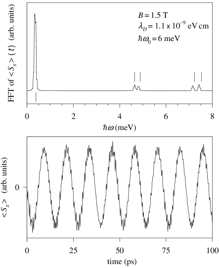
FIG. 1.: Real time simulation of the spin evolution following an initial rotation with $x$ axis. Shown is the $x$-component of total spin in time (lower) and energy (upper) domains. The vertical bars in the upper panel indicate the analytical energies with the Hamiltonian expanded to $O(\lambda_{D}^{3})$.

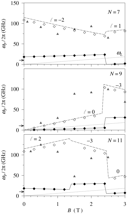
FIG. 2.: Systematics of SO precessional frequencies $\omega_{\cal P}$ as a function of magnetic field for two different values of the Dresselhaus parameter $\lambda_{D}$: in the analytical model (lines), and from the numerical calculation without (diamonds) and with Coulomb interaction (triangles with crosses). Solid lines and symbols correspond to $\lambda_{D}=0.4\times 10^{-9}\;{\rm eV}\;{\rm cm}$ while dashed lines, open symbols and crossed triangles to $\lambda_{D}=1.1\times 10^{-9}\;{\rm eV}\;{\rm cm}$. The dotted line shows the Larmor frequency. Also indicated is the $\ell$ value of the precessionally active orbital in the analytical model, which at a given $B$ is the same for both $\lambda_{D}$ values. The arrows on the vertical scale indicate the approximate lower frequency than can be obtained from the time simulation window of 100 ps.

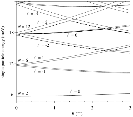
FIG. 3.: Energy level scheme as a function of the magnetic field for the same dot of Figs. 1 and 2 with a SO parameter $\lambda_{D}=1.1\times 10^{-9}{\rm eV}{\rm cm}$. The angular momentum for each level and the electron number at shell closures are indicated. The curves marked with thick dots and dashes indicate the precessionally active level for the electron numbers $N=7$, 9 and 11.

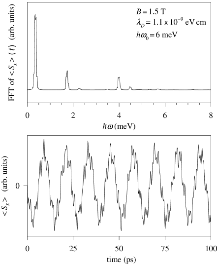
FIG. 4.: Same as Fig. 1 for the case with Coulomb interaction between electrons.

REFERENCES

- [1] S. A. Wolf, D. D. Awschalom, R. A. Buhrman, J. M. Daughton, S. von Molnár, M. L. Roukes, A. Y. Chtchelkanova, D. M. Treger, Science 294, 1488 (2001).
- [2] G. Salis, D. D. Awschalom, Y. Ohno, H. Ohno, Phys. Rev. B 64, 195304 (2001).
- [3] J. A. Gupta, D. D. Awschalom, X. Peng, A. P. Alivisatos, Phys. Rev. B 59, 10421 (1999); J. A. Gupta, D. D. Awschalom, Al. L. Efros, A.V. Rodina, preprint (cond-mat/0204235).
- [4] C. Durkan and M. E. Welland, Appl. Phys. Lett. 80, 458 (2002).
- [5] A. G. Aronov, Y. B. Lyanda-Geller, Phys. Rev. Lett. 70, 343 (1993).
- [6] O. Voskoboynikov, C. P. Lee, O. Tretyak, Phys. Rev. B 63, 165306 (2001).
- [7] W. Knap, C. Skierbiszewski, A. Zduniak, E. Litwin-Staszewska, D. Bertho, F. Kobbi, J. L. Robert, G. E. Pikus, F. G. Pikus, S. V. Iordanskii, V. Mosser, K. Zekentes, Yu. B. Lyanda-Geller, Phys. Rev. B 53, 3912 (1996).
- [8] I. D. Vagner, A. S. Rozhavsky, P. Wyder, A. Yu. Zyuzin, Phys. Rev. Lett. 80, 2417 (1998).
- [9] I. L. Aleiner and V. I. Fal’ko, Phys. Rev. Lett. 87, 256801 (2001).
- [10] M. Valín-Rodríguez, A. Puente, Ll. Serra, E. Lipparini, Phys. Rev. B (2002) in press; preprint (cond-mat/0206387).
- [11] M. Governale, preprint (cond-mat/0204410).
- [12] C. P. Slichter, Principles of magnetic resonance (Springer-Verlag, New York, 1990)
- [13] V. Fock, Z. Phys. 47, 446 (1928); C. G. Darwin, Proc. Camb. Phil. Soc. 27, 86 (1930). For a recent review see L. P. Kowenhoven, D. G. Austing, S. Tarucha, Rep. Prog. Phys. 64, 701 (2001).
- [14] D. Stein, K. v. Klitzing, G. Weimann, Phys. Rev. Lett. 51, 130 (1983).
- [15] A. Puente, Ll. Serra, Phys. Rev. Lett. 83, 3266 (1999).
- [16] M. Valín-Rodríguez, A. Puente, Ll. Serra, Phys. Rev. B 66, 045317 (2002).