Spin fluctuations, electron-phonon coupling and superconductivity in near-magnetic elementary metals; Fe,Co,Ni and Pd.

Abstract

An investigation of possibilities for superconductivity mediated by spin fluctuations in some elementary metals is motivated by the recent discovery of superconductivity in the hcp high-pressure phase of iron. The electronic structure, the electron-phonon coupling ($\lambda_{ph}$) and the coupling due to spin-fluctuations ($\lambda_{sf}$) are calculated for different phases and different volumes for four elementary metals. The results show that such possibilities are best for systems near, but on the non-magnetic side of, a magnetic instability. Fcc Ni, which show stable magnetism over a wide pressure range, is not interesting in this respect. Ferro- and antiferro-magnetic fluctuations in hcp Fe contribute to a relatively strong coupling in the pressure range where superconductivity is observed. The absence of fluctuations at large q-vectors makes fcc Pd only moderately interesting despite its large exchange enhancement for q=0. Fcc Co at high pressure ($\sim$ 0.5 Mbar) behaves as an improved version of Pd, where the fluctuations extend to larger q. The estimations of T_C, which reproduce the experimental situation in Fe quite well, suggest a measurable T_C for the high-pressure phase of fcc Co, while the estimate is lower for the ambient-pressure phase of fcc Pd.

E-mail address: thomas.jarlborg@physics.unige.ch

I Introduction.

Superconductivity has recently been reported in the hcp high-pressure phase of iron [1, 2]. The maximum of the superconducting transition temperature T_C, about 2 K, is in the middle of a pressure range of 150-300 kBar where superconductivity has been observed. Superconductivity is traditionally explained from electron-phonon coupling. This mechanism is sensitive to magnetic interactions and it would not be expected to find superconductivity in magnetic or almost magnetic materials. Alternatively, superconducting pairing can be mediated by spin fluctuations, and it might be that hcp Fe should be explained by this type of mechanism. since anti-ferromagnetic (AFM) instabilities are likely in the interesting pressure region. Further, some magnetic or nearly magnetic compounds have also been found to be be superconducting [3, 4], although the T_C’s are not very high. Both the electron-phonon coupling and ferromagnetic (FM) instabilities require a large electronic density-of-states, and the question is if superconductivity in such cases is the standard one caused electron-phonon coupling where T_C is limited by spin fluctuations, or if it is mediated by spin fluctuations in equal spin pairing (ESP). The fact that the superconductivity is found only in very pure samples is an indication that mechanism is the latter one, since impurity scattering is expected to interfere with ESP in a similar manner as magnetic impurities interfere with pairs which are hold together by electron-phonon coupling. In addition, theory indicates the pressure dependence of T_C in Fe is inconsistent with the mechanism of electron-phonon coupling [5, 6]. The recent discoveries of magnetic superconductors led to a renewed interest in theories of calculating the coupling strength, $\lambda_{sf}$, for spin fluctuations and how such fluctuations can mediate superconductivity [6, 7, 8, 9, 10, 11, 12, 13].

Superconductivity in some borocarbides, containing magnetic rare-earth elements is also surprising and interesting [14], but the situation is probably quite different from Fe and the compounds mentioned above, since the magnetic f-electron of the rare-earth atom is very localized and electronically isolated from the itinerant valence electrons. High-T_C copper oxides might be superconductors because of AFM fluctuations [15], but stripe-like spin waves may interact with phonons [16], and the mechanism not yet clear.

This work consider itinerant electrons in pure metals where magnetic fluctuations and superconductivity must coexist. Near-magnetic pure elements are particularly interesting in studies of superconductivity and magnetic fluctuations, both experimentally and theoretically. Non-compound elements can be made very pure without intrinsic defects caused by non-stoichiometry or vacancies in sub-lattices of compounds. This allows for ESP to develop without much interference from impurity scattering. Theoretically it is also preferable to consider pure metals over compounds. The electronic structure is simpler and especially for studies of extended AFM fluctuations by the method of frozen spin waves, it avoids the complication of having several types of sites where the local magnetic response can be different. In this work we study four metals, Fe, Co, Ni and Pd, which all are known to be ferromagnets or strongly enhanced paramagnets. Different phases are considered, and total energy calculations are used to determine the stability of hcp, fcc and bcc phases as function of pressure. A previous report considered FM and AFM spin fluctuations separately in hcp Fe, and it was concluded that the combined effect could explain the observed T_C [6]. This study is here extended to include the other three metals and where a weighting of different fluctuations are made, similar to what is made for phonons.

II Theory.

The electronic structures are calculated using the linear muffin-tin orbital method in the local spin density approximation (LSDA) [17, 18] and the generalized gradient approximation (GGA [19]) scheme, which includes non-local corrections to the potential. The basis set includes states up to $\ell$=3. The c/a-ratio in the hcp structures is fixed to 1.59 for all volumes. This is close to the calculated value within a wide pressure range for Fe [21], and a few tests with other ratios show that this choice is good also for Co. The number of k-points vary with the structure. For fcc and bcc it 505 and 506 points in the irreducible part of the Brillouin Zone (BZ), for hcp 252, and for the supercells with long wavelength AFM configurations we use the same density of points. The number of points is close to 500/n where n is the number of atoms per cell. The use of GGA instead of LSDA potential is known to be crucial for a correct description of the fcc vs. bcc stability of Fe, but other properties are not very different in the two types of density functional potentials [20]. A previous report on Fe used mainly LSDA for the calculations of $\lambda_{sf}$ [6]. Here, these results are complemented with calculations using GGA for the most interesting configurations in hcp iron. The magnetic coupling constants are similar (within $\sim$ 5 percent) to those calculated in the LSDA. As in ref. [21] it is found that two AFM configurations compete with the NM state in hcp iron at some pressures. The first (AFM-I) has opposite polarization on each alternate z-plane layers, while the second (AFM-II) has opposite polarization on each layer perpendicular to the x-axis. The results for Ni, Co and Pd are new, and only results from GGA calculations are reported.

The electron-phonon coupling parameter $\lambda_{ep}$ is calculated from the electronic structure;

$$\lambda_{ep}=NV^{2}/M\omega^{2}=NV^{2}/K$$ (1)

where $N$ is the density of states at $E_{F}$, $M$ the atomic mass, $\omega$ a phonon frequency and $K$ a force constant. The latter is related to the change of total energy $E$ due to an atomic displacement $r$, $K=d^{2}E/dr^{2}$. The Hopfield parameter $NV^{2}$ contains $V$, the Fermi surface (FS) average of the matrix element $<\psi_{k}(dv(r)/dr)\psi_{k}>$, the first order change in energy due to the displacement, where $\psi_{k}$ is the wave function at the k-point $k$, and $v(r)$ is the potential. For elementary metals it is a good approximation to calculate $V$ within the rigid muffin-tin approximation RMTA [22], which in the case of LMTO band results is slightly modified to the rigid Wigner-Seitz (WS) approximation [23]. The alternative to calculate $V$ from the change in band energies, $\varepsilon_{k}$, when the structure is deformed as in a ’frozen’ phonon, demands a larger computational effort since several large supercell calculations are needed to map out representative phonons. The force constant is fitted to the experimental value of the Debye temperature $\Theta_{D}$ at zero pressure, and then scaled to other volumes by the calculated bulk modulus [24]. This scaling is assumed to be valid also between the hcp and bcc phases for Fe and between the hcp and fcc phases of Co. The calculated values of $\lambda_{ep}$ at equilibrium volumes agree well with independent results for the elements considered here [25, 26]. This is despite the use of Wigner-Seitz cells instead of non-overlaping Muffin-Tin spheres in the evaluation of the matrix elements.

Interesting spin fluctuations occur near magnetic instabilities when only a small energy is needed to excite a magnetic wave in the material. The energy is zero at the magnetic instability and it can be very low close to the instability, lower than the energy of typical phonon energies. It is also noted that spin fluctuations can be the result of a divergence of the generalized susceptibility, $\chi(q,\omega)$, implying that Fermi surface nesting for critical values of $q$ is partly responsible for the divergence. This is also the case for phonon softening when some $q$-modes become unstable. Phonons with $q$ outside the BZ have no sense, since the wave length cannot be shorter than two interatomic distances. Spin- or charge- density waves with wavelengths shorter than the size of an atom can be imagined, but if they were important they should probably exist already on the level of a single atom, before the scattering within several sites in a lattice can set up a FS and nesting. Since the structure always seems to be important for the properties of a material, we assume that fluctuations corresponding to $q$-vectors outside the BZ are not important. Thus, we consider only ”soft” spin fluctuations with energies and wavelengths which are similar as for phonons. If adiabatic conditions and the Migdal theorem are valid for phonons they should also be valid for soft spin fluctuations.

As was pointed out in a previous work [6], the analogies between soft spin-wave excitations and phonons can be utilized. A spin wave with a moment $m$ and a phonon with lattice-displacements ”$r$” both generate perturbations of the potential, although the perturbations are of different kinds. Magnetic moments and the spin-polarized perturbation of the potential have spherical symmetry within each site, except for very short wave lengths of the spin waves. The matrix elements $V$ are mainly monopolar, which couple electronic states of equal $\ell$. Atomic displacements generate mainly an asymmetric (and non-polarized) perturbation of the potential at each site. Ionic compounds, where the displacements are associated with large Madelung shifts, can have some monopolar coupling [27]. But here, in neutral pure elements, the matrix element $V$ is dominantly dipolar with the selection rule $\ell-\ell^{\prime}=\pm 1$. In addition there is a technical difference of how the frozen phonon and spin wave calculations are made. By applying a magnetic field $\xi$ one obtains a magnetic moment $m$ in frozen spin wave configurations. However, the displacements in frozen phonon calculations are imposed instead of being a result of an applied force. This difference would disappear if we did so-called ”fixed-spin-moment” (FSM) calculations instead of applying the magnetic field. The total energy in such case is the free energy for the configuration with the fixed moment, while with imposed field the free energy is the total energy plus the term field times moment. In practical calculations we prefer the method with applied fields which is simple to use both for FM and AFM cases.

The calculation of mass enhancement due to FM or AFM spin fluctuations, $\lambda_{sf}$, is analogous to that for phonons, but with ”$r$” replaced by ”$m$”.

$$\lambda_{sf}=NV^{2}/K=N<\psi_{k}(dv(r)/dm)\psi_{k}>^{2}/(d^{2}E/dm^{2})$$ (2)

Calculations for spin wave excitations with general q-vectors require supercells, as in the case of frozen phonon calculations. The calculations are made for two different configurations, one with an applied field and one without, to give two band structures and two magnetizations. If the changes of the free energy $(E)$ are harmonic, i.e. quadratic functions of the induced magnetic moment, we have $E_{\xi}=E_{0}+Jm^{2}$ where $m$ is the moment (induced by the field $\xi$) per atom. The constant $J=\frac{1}{2}d^{2}E/dm^{2}=(E_{\xi}-E_{0})/m^{2}$ is calculated from spin polarized results, where the applied fields range from 1 to 10 mRy. The local Stoner enhancement, $S$, is defined as $(\epsilon_{\xi}-\epsilon_{0})/\xi$, where $\epsilon_{\xi}$ is the increase of the exchange splitting at an atom (obtained from the logarithmic derivative of the d-band) induced by the field $\xi$. (K-dependent Stoner enhancements can be obtained by taking the exchange splitting from the band energies at each k-point.) The $S$-values are generally smaller for large $\xi$, indicating some aversion against large moments and non-harmonic variations of $J$ as function of field.

The monopolar matrix element $<\psi_{k}dv\psi_{k^{\prime}}>$ can be calculated directly from the change in the spin part of the potentials between the two cases, with and without field. This permits calculation of the anisotropy of the coupling, $\lambda(k,k^{\prime})$, which is needed in Eliashberg theory to determine if the superconductivity is s-, p-wave or of some higher symmetry. In this work we do not determine the anisotropy, but only the FS average of $\lambda(k,k)$. In this case it is convenient to determine the matrix element directly from the change in band energies, simultaneously to the ’frozen spin wave’ determination of the change in total energy. Hence, $<\psi_{k}dv\psi_{k}>^{2}=(\varepsilon_{k}^{m}-\varepsilon_{k}^{0})^{2}$, where $\varepsilon_{k}^{m}$ is the band energy at point $k$ for the configuration belonging to $m$. In the harmonic limit we obtain finally;

$$\lambda_{sf}=N<(\varepsilon_{k}^{m}-\varepsilon_{k}^{0})^{2}>_{FS}/2(E_{m}-E_{0})$$ (3)

Here $<~{}>_{FS}$ means a FS average. The matrix element is more efficient for FM than for AFM fluctuations, because a FM field applied in a system where one band is dominant at $E_{F}$, will split all bands about equally. The same difference $(\varepsilon_{k}^{m}-\varepsilon_{k}^{0})$ will appear almost everywhere over the FS. For induced AFM configurations it is more difficult to visualize these differences. Positive and negative differences are likely, which means that small differences should exist at some sections of the FS and make the averaged matrix element smaller.

The energy of the FM and AFM fluctuations, $\hbar\omega_{sf}$, is estimated from a Heisenberg model, where the parameter $J$, the exchange integral, is the maximum amplitude of the spin wave [28]. For ferromagnetic fluctuations it has been proposed that $\hbar\omega_{sf}=1/(4NS)$ [13]. The corresponding property in the present approach is $J/4$.

In order to make the calculations of superconductivity mediated by spin fluctuations analogous to that mediated by phonons, one needs to include a number of representative $q$-vectors. We consider FM fluctuations ($q$=0) and a few AFM fluctuations with $q$ at the zone boundary. For fcc Co we calculate intermediate $q$ by use of supercells with up to 8 atoms. The results from the intermediate $q$ vectors show no surprises, but the coupling and $J$ are between the values for large and zero $q$. This indicates that no drastic effects from the FS are seen, but it can not be excluded that effects from nesting at particular $q$-vectors can be missed by the method of supercell calculations. It is as for frozen phonon calculations, where one assumes a smooth variation between the values calculated at a few $q$-points. If a special mode-softening is known initially it can be studied carefully.

The strong coupling parametrization of the Eliashberg theory for electron-phonon coupling by McMillan [29] contains the weighted averages of the coupling $\lambda$ and the frequency $\omega_{log}$.

$$\lambda=2\int\alpha^{2}F(\omega)\frac{d\omega}{\omega}$$ (4)

$$\omega_{log}=exp(\frac{2}{\lambda}\int\frac{ln\omega}{\omega}\alpha^{2}F(\omega)d\omega)$$ (5)

With the few number of spin waves we replace the integration by a summation over $q$-points ”$i$” with relative weights $w_{i}$. The density-of-state contribution $\alpha^{2}F(\omega_{i})$ from mode $i$ is contained in the value $\lambda_{i}$, which is defined $2\Delta\omega_{i}\alpha^{2}F(\omega_{i})/\omega_{i}$ for a single mode.

$$\lambda=\sum_{i}w_{i}\lambda_{i}$$ (6)

$$\omega_{log}=exp(\frac{1}{\lambda}\sum_{i}ln\omega_{i}w_{i}\lambda_{i})$$ (7)

Superconductivity based on electron-phonon interaction is easily destroyed by magnetic impurities and magnetic fluctuations. The spin-splitting of the potential leads to an attraction between electrons of equal spin and compete with the attractive interaction between Cooper pairs. Effects from impurities are not included, but for the effect from spin fluctuations we use the Daams et al modification [30] of the McMillan formula due to $\lambda_{sf}$, so that $\lambda_{eff}=\lambda_{ep}/(1+\lambda_{sf})$ will replace $\lambda_{ep}$.

$$k_{B}T_{C}=(\frac{\hbar\omega_{log}}{1.2})exp(\frac{-1.04(1+\lambda_{eff})}{(\lambda_{eff}-\mu^{*}(1+0.62\lambda_{eff}))})$$ (8)

In addition, with $\mu^{*}$=0, the expression becomes formally very similar to the expression for T_C by paramagnon coupling, see below.

For superconductivity mediated by spin fluctuations the situation is reversed, so that non-magnetic impurities and strong electron-phonon coupling reduce T_C. This is because the pairing is between electrons of equal spins, and scattering with impurities or phonons will reduce the spin-splitting of the local potential. For estimating the superconducting transition temperature we use a simplified version of the weak coupling BCS-like formula for paramagnon coupling [31, 10].

$$k_{B}T_{C}=({\hbar\omega_{sf}}/{1.2})exp({-(1+\lambda_{ep}+\lambda_{sf}^{0})/\lambda_{sf}^{1}})$$ (9)

The calculated enhancement parameter due to spin fluctuations is mainly considered to be of p-character, $\lambda_{sf}^{1}$, although we have not investigated the $(k,k^{\prime})$-dependence over the FS. The s-wave fraction of the total $\lambda_{sf}$, $\lambda_{sf}^{0}$, is expected to be small, but it can be more important at larger q, when the perturbing potential has stronger dipolar character, as in the case of atomic displacements in electron-phonon coupling. The s-part should also contain a contribution from transverse fluctuations [10]. Two extreme values of $\lambda_{sf}^{0}$ are assumed, either that $\lambda_{sf}^{0}$=$\lambda_{sf}^{1}$ or that $\lambda_{sf}^{0}$=0, in order to obtain the range of extreme values on T_C. The second choice turns out to give a $T_{C}$ of a reasonable amplitude compared to what is measured for hcp Fe, while the T_C is about half as large if the s-part is assumed to be equal to the p-part. It is obvious that with the various approximations it is not possible to give precise values for $T_{C}$, but the values should be taken as a possible range of T_C in the different materials. The result for hcp Fe serves as a calibration; since the T_C and its pressure variation agree quite well with experiment, there is some hope that the same method can be used as a guidance for the other materials, especially for fcc Co where no experimental data are known.

III Results.

The exchange enhancement is defined as the increase of the exchange splitting of the d-band divided with the energy of the applied magnetic field [32]. This definition is natural for FM cases and it leads to the usual Stoner enhancement for paramagnets. We also define a local exchange enhancement for AFM configurations, when the field is applied differently on different sites. The results show that these exchange enhancements are largest when the material is close to, but on the non-magnetic side of, a magnetic (FM or AFM) instability. As the volume is decreasing in a magnetic system one will find a critical volume where the (local) moments disappear at a certain volume. The local exchange enhancement will be infinite at the critical volume and still large for decreasing volumes. But within the region where the volumes are larger than the critical volume, the exchange enhancement drops rather quickly. It is as if the minimum of the total energy as function of the moment in a magnetic system is deeper than in a non-magnetic one, and the additional fields will not have a large influence on the moment. In other words, non-magnetic materials are magnetically ”softer” than the materials which already have a magnetic ground state. A consequence of this is that $\lambda_{sf}$ will behave asymmetrically as function of pressure around the critical volume, so that it will be lower in magnetic region than in non-magnetic one. This is at least the results from the calculations for several configurations in these pure elements. One may add that we have not considered more than the three most common structures. The calculations can not exclude that other structures may appear at high pressure.

A Nickel.

The calculations for fcc-, bcc- and hcp-structures of Ni show that the FM state is very persistent. This is for pressures varying from zero up to more than 3 Mbars, or when the volume is compressed to 45 $(a.u.)^{3}$/atom from the equilibrium volume of 73 $(a.u.)^{3}$/atom. Only the bcc structure has a vanishing moment for volumes below about 62 $(a.u.)^{3}$/atom, but the total energy is always larger than for magnetic fcc, about 4 mRy/atom within the whole range of volumes. The hcp structure is FM with a moment ranging from 0.6 to 0.49 $\mu_{B}$/atom in this range of volumes. This is very similar to fcc, where the range of $m$ is from 0.62 to 0.48 $\mu_{B}$/atom. However, the total energy of the hcp phase is 3-5 mRy/atom larger than in fcc. The results suggest that NM bcc should be stable over FM hcp at large pressure, but FM fcc is the most stable structure everywhere.

These facts, the stability of the FM fcc phase, and the low values of exchange enhancements and $\lambda_{sf}$ for magnetic phases, make together that Ni seems not interesting as a candidate for superconductivity mediated by spin fluctuations. The NM bcc phase could have large $\lambda_{sf}$ near the magnetic instability for a pressure of the order 0.5 Mbar, but since it is not the most stable phase we refrain from making detailed calculations.

B Iron.

Several results for Fe in a previous publication [6] are complemented by adding a few GGA results. The FM bcc phase is stable for volumes larger than 72 $(a.u.)^{3}$/atom, while NM hcp is stable for lower volumes, see fig. 1. Two AFM configurations are stable for hcp. The AFM-I configuration (when the moments alternate along the z-axis) is stable only at large volumes, while the AFM-II configuration (alternation along the x-axis) is stabilized just below the critical volume where bcc is stable. This is in agreement with independent calculations, where interpretation of Raman shifts lends support to the existence of AFM order [33]. However, the moment is small and the total energy is almost the same for the NM hcp structure for volumes smaller than 72 $(a.u.)^{3}$/atom [6]. The calculation of $\lambda_{ep}$ is done in the rigid WS approximation with the phonon denominator scaled by Debye temperature and the P-dependence of the bulk modulus. The $\lambda_{ep}$ for the bcc structure agree with previous RMTA calculations [25, 26]. The values for the hcp phase are somewhat smaller than in ref. [5], with a similar relative decrease as function of pressure (P). This is mainly because of the difference in force constant $K$, while the matrix elements for the electron phonon coupling are similar.

The calculations of $\lambda_{sf}$ and T_C are done following the procedures described above using the previous results from FM and the two AFM configurations [6]. The weights in the summations for $\lambda_{sf}$ and $\omega_{log}$ (1/5, 1/5 and 3/5 for FM, AFM-I and AFM-II, respectively) are obtained from the q-values of the spin configurations. The results are given in Table 1. The variation of $\lambda_{ep}$ is continuous between the largest and smallest volume. This is true also for $\lambda_{sf}$ and $\omega$ for FM fluctuations. The FM instability occurs well beyond the range of volumes considered here where the Stoner enhancement never is larger than 3.2. The corresponding values $\lambda_{sf}$ (and $\omega$) for the two AFM configurations show pronounced peaks (dips) near the critical volumes for the magnetic instabilities. The local Stoner factors diverge at these volumes. These instabilities are reflected in the averaged values of $\lambda_{sf}$ and $\omega_{log}$, so that together with the contribution from FM fluctuations there are conditions for superconductivity near two volumes, see fig. 2. The calculated T_C agrees well with experiment when $\lambda_{sf}^{0}$ is assumed to be zero, with a maximum of about 1.2 K just below the volume at which the hcp phase becomes stable and with T_C approaching zero at larger pressures. A second peak in $T_{C}$ is seen at larger volume, where the AFM-I becomes unstable. However, this can not be tested experimentally since the bcc structure is stable at such volumes. Also hypothetically, it is possible that strong FM fluctuations may give superconductivity at even larger volumes. As a comparison we also calculate the T_C based on electron-phonon coupling with reduction due to $\lambda_{sf}$, using the formula of Daams et al [30]. With $\mu^{*}$=0, T_C is about 1.0 K just after the bcc-hcp transition at the volume 70 $(a.u.)^{3}$/atom. This value is in reasonable agreement with experiment, but the reduction with pressure is too slow in comparison with experiment. At 58 $(a.u.)^{3}$/atom T_C is still 0.3 K. This corresponds to a rather smooth reduction of T_C from 1.0 to 0.3 K within a pressure range of $\sim$ 700 kBar, compared to a confinement of T_C within 200-300 kBar from spin fluctuations and within $\sim$ 150 kBar experimentally [1]. Thus, from the pressure dependence of T_C it can be concluded that superconductivity is more likely to be mediated by spin fluctuations. A similar conclusion was reached by Mazin et al [5].

The good agreement with experiment for the amplitude of T_C could be accidental. Many approximations are used and the statistics for the q-average is poor. On the other hand, the relative variations with pressure should be more reliable, since the procedure for calculating T_C always is the same. This motivates a study of Co and Pd with the same procedure in order to verify if Co could be superconducting at high pressure and if fcc Pd, with its large exchange enhancement, will incorrectly appear as a superconductor by this theory.

C Cobalt.

The stable phase of Co at zero pressure is FM hcp with a moment of 1.59 $\mu_{B}$/atom when volume is 73.1 $(a.u.)^{3}$/atom. The total energy of the NM hcp state is 15.5 mRy/atom higher at the same volume, which is close to the experimental volume at equilibrium. Figure 3 shows the total energies from FM and NM GGA calculations of the three structures, and the FM moments are shown in fig. 4. The bcc structure is magnetic within a wide range of pressures, but its total energy is considerably above those of fcc and hcp, and the bcc phase is not of interest here. It is seen in fig. 3 that the fcc structure becomes stable (over hcp) at a volume near 58 $(a.u.)^{3}$/atom. The pressure at this volume is about 0.8 and 0.7 Mbar for hcp and fcc, respectively. The transition volume is below the volume (about 60 $(a.u.)^{3}$/atom) where fcc becomes NM. Therefore, from the experience with Fe it is expected that the Stoner enhancement and $\lambda_{sf}$ for FM fluctuations become very large at volumes just below the FM instability. In spin polarized calculations near the critical volume for the FM instability it is possible to find metastable low- and high-moment states with almost degenerate total energies. This leads to large non-linear Stoner enhancements so that S are large at large field. The S-values vary from 4 at the volume 54 $(a.u.)^{3}$/atom when the applied field is 1 mRy to 28 at 59 $(a.u.)^{3}$/atom for the field of 2 mRy. As was discussed earlier, it is generally easier to find large $\lambda_{sf}$ for FM than for AFM fluctuations [6], and here we obtain very large values, from 0.9 to 2.4 within this range of volume and field. This is much larger than for FM fluctuations in hcp Fe, where the FM instability is outside the considered range of volumes. The AFM instabilities are within the range volumes, but the corresponding $\lambda_{sf}$ is rather modest, since the matrix element for AFM fluctuations is not so efficient.

The FM Stoner factors on the magnetic side of the transition are much smaller, about 1.7, and typical $\lambda_{sf}$ is of the order 0.1. This agree with the findings for AFM fluctuations in Fe, and FM fluctuations in hcp Co. The latter is magnetically ordered within the entire range of volume where it is the stable phase, and it is not promising for superconductivity.

A few AFM configurations are made for two volumes of fcc Co just below the volume where FM disappears, at 56 and 59 $(a.u.)^{3}$/atom. The applied field is used to impose AFM modulations in the x-direction for different wave lengths, corresponding to 2, 4 and 8 atoms in supercell calculations. (The field amplitude, 1 or 2 mRy, is the same on each site so that the wave is step-like rather than sinus-like.) The local Stoner enhancements are lower than for the FM case at equivalent volumes. For the shortest AFM wave $S$ is 2.3 compared to 28 for the FM configuration. For the longest wave there are 4 layers of atoms where the field is of the same sign. Thus, the two in the middle are surrounded by sites of the same polarization and $S$ is 10 within this region of ”local” FM order. But the two atoms at the edge of the 4-layer atoms, have one neighbor with reversed polarization, and $S$ is lower, about 6, for these sites. The coupling $\lambda_{sf}$ is relatively small for all of the AFM configurations. It varies from 0.26 to 0.09 and to 0.03 for the longest, the intermediate and the shortest wave, when the volume is 59 $(a.u.)^{3}$/atom. These values are reduced further to 0.07, 0.06 and 0.03, when the volume is 56 $(a.u.)^{3}$/atom.

Some values the electron-phonon coupling were calculated for the hcp phase. At large volume this phase is FM and the coupling is dominated by the minority band which has the largest DOS. At the equilibrium volume $\lambda_{ep}$ is 0.19 for the minority band and 0.05 for the majority band, while at 54 $(a.u.)^{3}$/atom, when the magnetism is strongly reduced, the amplitudes are reversed, 0.25 and 0.20. This is because of a large increase of the majority DOS. A $\lambda_{ep}$ of this order should make superconductivity possible if spin fluctuations are absent. However, hcp Co is still magnetic at this volume and the fact that fcc is the stable phase at this volume makes it not very interesting to study superconductivity based on electron-phonon coupling. Instead, we calculate $\lambda_{ep}$ for the NM fcc phase in order to investigate whether it can give superconductivity mediated by phonons or if it will prevent superconductivity mediated by spin fluctuations. The calculated values of $\lambda_{ep}$ are rather stable as function of volume, about 0.41. This is for a $\Theta_{D}$ of 550 K at the volume 56 $(a.u.)^{3}$/atom. The calculation of T_C is made as for Fe. If the reducing effect from the (q-weighted) $\lambda_{sf}$ is included one obtains 0.1 K at 56 $(a.u.)^{3}$/atom and 0.01 at 59 $(a.u.)^{3}$/atom. Without influence of spin fluctuations we obtain 0.56 and 0.3 K.

The estimation of T_C from spin fluctuations are done as in the case of Fe, using the q-weighted results in table 2, with the reducing effect from electron-phonon interaction and with two assumptions for $\ell=0$ part of $\lambda_{sf}$ (either 0 or equal to the $\ell=1$ part). The results are 0.2 and 0.06 K, respectively, at the smallest of the two volumes, while 1.1 and 0.4 K, respectively, at the large volume.

There are many approximations and uncertainties behind these values, but since the method is identical to the method used for Fe, where the experimental amplitude is fairly well reproduced or even underestimated, there is some hope that superconductivity could be observed in Co just after the hcp-to-fcc phase transition. The calculations predict the transition pressure to be very high, of the order 700 kBar, but as seen in fig 3, a small error in the relative position between the total energy curve will shift the transition volume (and pressure) a lot. If the critical pressure in reality were even higher, it would be less likely to expect superconductivity mediated by spin fluctuations, because the material would be further away from the instability point when the fcc structure becomes NM. The critical volume for the FM to NM transition is not as sensitive because if does not depend on the relative differences between the total energy of two structures. However, the magnetic transition for the fcc phase is diffuse and extends over some interval of volumes, where non-linear effects and metastable states are found. Therefore, if the hcp to fcc transition turns out to happen at larger volume, there is some margin for having larger values of $\lambda_{sf}$ and T_C, than what has been calculated here. This is since the volume for the onset of FM in the fcc structure appears to around 60 $(a.u.)^{3}$/atom, while the largest volume for the calculation of $\lambda_{sf}$ is 59 $(a.u.)^{3}$/atom. All partial values of the enhancements and $\lambda_{sf}$, FM or AFM, tend to increase when the system is closer to the critical volume, but non-linear effects make the supercell calculations more difficult.

Some differences with Fe can be noted. The structures are different and it is difficult to say if this somehow will annihilate the advantages coming from the fact that the method of calculation is as identical as possible for the two systems. The relative weights between FM and AFM fluctuations are also different. Fe is far from the FM instability, but there two stable AFM configurations are close and fluctuations from them contribute to the final $\lambda_{sf}$. No AFM instability is found in these calculations for fcc Co. It is the FM case which dominates, with a Stoner factor which at the largest volumes becomes considerably larger than in Pd. Since Pd at ambient pressure also is of fcc structure, has a large exchange enhancement, but has not been found superconducting, one could test the same method for Pd.

D Palladium.

For Pd we consider only the fcc phase at the experimental lattice constant when the volume is 98.5 $(a.u.)^{3}$/atom. The electon-phonon coupling is calculated to be 0.36 for a $\Theta_{D}$ of 274 K. The Stoner enhancement for FM configuration is 5.7, in agreement with earlier estimations using LSDA [32]. This enhancement is smaller than the largest values calculated for Co, which implies that the hypothetical FM instability in Pd would require a considerable increase in volume. Also the local enhancements for the AFM configurations are smaller than the corresponding values for Co. From the calculations using 2 and 4 atoms/cell $S$ is 1.7 and 1.9, and for the two inequivalent sites in the 8 atom cell the values are 2.4 and 3.6. The coupling $\lambda_{sf}$ for the three AFM cases are of the order 0.02 to 0.14 from the shortest to the longest wave, while for the FM case it is calculated to be between 1.4 and 1.8 depending on the amplitude of the applied field. Thus, the enhancements in Pd is comparable to the result for Co calculated for the smallest volume. The q-averaging is done for the equivalent modes as for Co, and the results are $\lambda_{sf}$=0.15 and $\omega$=13 mRy.

The estimate for T_C is below 0.01 K for superconductivity mediated by electron-phonon coupling (but limited by spin fluctuations), and between 0.08 and 0.03 K for the two assumptions of $\lambda_{sf}^{0}$ in the calculation of T_C from ESP (and limited by electron-phonon coupling). The latter values are smaller than the results for two volumes of fcc Co, and T_C is very low despite the large exchange enhancement of Pd. The reason is that the large exchange enhancement is not extending to large q-values, and the averaged $\lambda_{sf}$ is not large enough for superconductivity. The material does not support spin excitations where adjacent atoms have different polarization. This is very different from hcp Fe where opposite polarization on near neighbors even give stable AFM configurations. If the volume of Pd were $\sim$ 5 percent larger, one could expect results similar to what is calculated for fcc Co. The reduction of enhancements at large q is crucial for an understanding of the small T_C or even absence of superconductivity. A calculation based only on the standard Stoner enhancement (at q=0) would not be correct. A recent work suggests that spin-orbit coupling can suppress superconductivity in Pt [34]. One may speculate that such an effect should be more evident in Pd than in Co because of the relative strengths of the spin-orbit coupling.

IV Conclusion.

Two possibilities for superconductivity in four exchange enhanced metals have been investigated by calculations of the coupling constants for electron-phonon coupling and spin fluctuations. The method for calculating $\lambda_{ep}$ and the corresponding T_C has been quite successful in many studies during the last decades, while the method for calculating $\lambda_{sf}$ is new and needed some testing. Both methods include approximations and one should not rely too much on to the absolute values of T_C, but look more at the relative variations among the different cases and different pressures. Despite these precautions, it seems clear that superconductivity based electron-phonon coupling is unlikely in Pd, Co and Ni. This is because of the limitation of T_C coming from spin fluctuations or from stable magnetic moments, and from the rather modest values of $\lambda_{ep}$. Hcp Fe could have a reasonable T_C, but the agreement with experiment is poor for the pressure dependence when electron-phonon coupling determines T_C.

The results for T_C based on ESP are partly a test of the method, partly a prediction. The experimental situation in hcp iron is surprisingly well reproduced, both the amplitude of T_C ($\sim$ 1.2 K) and its variation with pressure. This result indicate that a representative q-point average of $\lambda_{sf}$ has to be calculated. The calculation for fcc Pd pass the test as well, since T_C is very low ($\sim$ 0.08 K) despite its large Stoner factor. Again, this is the result only when several configurations are weighted together. The calculations indicate that a NM fcc phase of Co becomes stable at a high pressure of the order half a Mbar. Here, Co behaves as an improved version of Pd with larger enhancements, but with similar relative variation as function of q. The improved conditions for superconductivity from spin fluctuations give a T_C of the order 1 K.

These calculations do not include considerations of defects. Since superconductivity due to FM fluctuations is sensitive to impurity scattering [35], it is possible that lattice defects, induced in pressure experiments near a structural transition, can suppress $T_{C}$. It is not yet clear if experimental conditions can be improved to make T_C higher in hcp Fe or even in Pd. The reduction of $T_{C}$ compared to $T_{C}$ itself is proportional to $v_{F}/(\ell\Delta)$, where $\ell$ the impurity scattering length, $\Delta$ the superconducting energy gap and $v_{F}$ is the Fermi velocity [10]. Knowledge of the q-dependence of the destructive effect from defects on $\lambda_{sf}$ or ESP should be useful, since this can make a difference between Fe and Co (and Pd). The FM fluctuations are relatively important in the latter two metals of fcc structure. This is in contrast to hcp Fe, where the AFM fluctuations have a large weight. Calculations for supercells containing a defect give information about how much a defect will hamper the development of FM or AFM spin waves. The real space interpretation of the AFM results for Pd is that it is not easy for neighboring sites to have different magnetization. If so, it should also be difficult for a FM moment to develop near to a non-magnetic impurity in Pd, which could make this material more sensitive to impurities than Fe. In the absence of full calculation with impurities one can also note that from the dispersion of spin waves it follows that fluctuations with intermediate $q$ are mobile with large values of the group velocities. They may interfere with defects, while waves with $d\omega/dk\sim 0$ (as for a purely FM fluctuation) can develop easier between defects. Co is an intermediate case between Fe and Pd even without considerations of defects, still with possibilities for a measurable T_C.

TABLE I.: Volume per atom, partial and q-weighted $\lambda_{sf}$ and $\omega_{sf}$ (in energy units) for hcp iron. The weights are 0.2 0.2 and 0.6 for FM, AFM-I and AFM-II, respectively. The electron-phonon coupling decreases continuously from 0.37 for the largest volume to 0.14 for the smallest volume.

V		$\lambda_{sf}$				$\omega$		$\omega_{log}$
	FM	AFM-I	AFM-II	tot	FM	AFM-I	AFM-II	tot
$(a.u.)^{3}$					mRy	mRy	mRy	mRy
79.2	0.61	0.08	0.02	0.15	3.2	6.3	25	4.1
76.8	0.54	0.61	0.03	0.25	3.7	0.5	20	1.6
74.5	0.43	0.30	0.04	0.17	4.0	0.9	26	2.8
70.1	0.32	0.14	0.14	0.18	5.0	2.1	3.0	3.4
67.0	0.28	0.09	0.26	0.23	5.5	3.0	1.4	1.8
66.0	0.26	0.06	0.21	0.19	5.8	3.5	1.3	2.0
62.1	0.20	0.03	0.10	0.11	7.2	4.8	2.1	3.5
58.5	0.15	0.02	0.06	0.07	11.	6.2	3.2	5.7

TABLE II.: Volume per atom, $\lambda_{ep}$, partial and total q-weighted $\lambda_{sf}$, and total $\omega_{log}$ (in energy units) for spin fluctuations in fcc Co at two volumes, and in fcc Pd (last line). The weights are 1/16, 3/16, 6/16 and 6/16 for FM, and the 3 different AFM configurations ordered according to the wave length (2 4 or 8 atoms).

V	$\lambda_{ep}$			$\lambda_{sf}$			$\omega_{log}$
$(a.u.)^{3}$		FM	AFM-2	AFM-4	AFM-8	tot	mRy
56	0.42	1.6	0.03	0.06	0.07	0.18	12.8
59	0.41	2.4	0.03	0.10	0.26	0.27	5.6
99	0.36	1.4	0.02	0.04	0.15	0.16	13.1

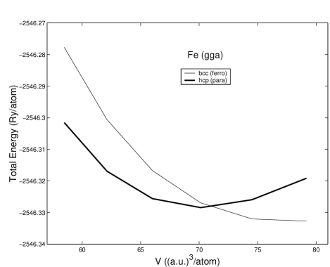
FIG. 1.: Calculated total energies for paramagnetic hcp (heavy line) and ferromagnetic bcc (thin line) iron using the GGA potential.

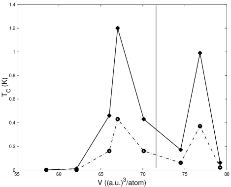
FIG. 2.: Calculated $T_{C}$ in hcp iron from eq. 9 using the values $\lambda_{ep}$ and the weighted values of $\lambda_{sf}$ and $\omega_{log}$ in Table 1. The full line is for $\lambda_{sf}^{0}=0$ and the broken line for $\lambda_{sf}^{0}=\lambda_{sf}^{1}$. To the right of the vertical line is the stable structure bcc (and T_C=0) according to the calculations. Superconductivity has been observed with $T_{C}$ below 2 K in a pressure range of about 150 kBar starting near the bcc-hcp transition pressure [1].

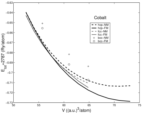
FIG. 3.: Calculated total energies using GGA potential as function of the volume for hcp, fcc and bcc Co.

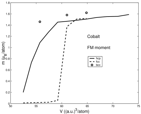
FIG. 4.: Magnetic moments calculated using GGA potential for hcp, fcc and bcc Co.

REFERENCES

- [1] K. Shimizu, T. Kimura, S. Furomoto, K. Takeda, K. Kontani, Y. Onuki and K. Amaya, Nature (London) 412, 316 (2001).
- [2] D. Jaccard, A. Holmes, G. Behr and Y. Onuki, Phys. Lett. A, (to appear) (2002).
- [3] S.S. Saxena, P. Agarwal, K. Ahilan, F.M. Grosche, R.K.W. Haselwimmer, M.J. Steiner, E. Pugh, I.R. Walker, S. R. Julian, P. Monthoux, G.G. Lonzarich, A. Huxley, I. Sheikin, D. Braithwaite and J. Flouquet, Nature (London) 406, 587 (2000).
- [4] C. Pfleiderer, M. Uhlarz, S.M. Hayden, R. Vollmer, H.V. Löhneysen, N.R. Bernhoeft and G.G. Lonzarich, Nature (London) 412, 58 (2001).
- [5] I.I. Mazin, D.A. Papaconstantopoulos and M.J. Mehl, Phys. Rev. B 65, 100511, (2002).
- [6] T. Jarlborg, Phys. Lett. A300, 518, (2002).
- [7] N.F. Berk and J.R. Schrieffer, Phys. Rev. Lett. 17, 433, (1966).
- [8] S. Doniach and S. Engelsberg, Phys. Rev. Lett. 17, 750, (1966).
- [9] T. Jarlborg, Solid State Commun. 57, 683 (1986).
- [10] D. Fay and J. Appel, Phys. Rev. B 22, 3173 (1980).
- [11] C.P. Enz and B.T. Matthias, Science 201, 828, (1978).
- [12] G. Santi, S.B. Dugdale and T. Jarlborg, Phys. Rev. Lett. 87, 247004, (2001).
- [13] I.I. Mazin and D. Singh, Phys. Rev. Lett. 79, 733 (1997).
- [14] P.C. Canfield, P.L. Gammel and D.J. Bishop, Phys. Today 51, No. 10, 40 (1998).
- [15] D. Pines, Z. Phys. B 103, 129, (1997).
- [16] T. Jarlborg, Phys. Rev. B64, 060507(R), (2001).
- [17] O. K. Andersen, Phys. Rev. B 12, 3060 (1975) ; T. Jarlborg and G. Arbman, J. Phys. F 7, 1635 (1977).
- [18] W. Kohn and L.J. Sham, Phys. Rev. 140, A1133, (1965); O. Gunnarsson and B.I Lundquist, Phys. Rev. B13, 4274, (1976).
- [19] J.P. Perdew and Y. Wang, Phys. Rev. B33, 8800, (1986).
- [20] E.G. Moroni and T. Jarlborg, Europhys. Lett. 33, 223, (1996).
- [21] G. Steinle-Neumann, L. Stixrude and R.E. Cohen, Phys. Rev. B 60, 791 (1999).
- [22] G.D. Gaspari and B.L. Gyorffy, Phys. Rev. Lett. 28 801 (1972).
- [23] M. Dacorogna, T. Jarlborg, A. Junod, M. Pelizzone and M. Peter, J. Low Temp. Phys. 57, 629 (1984).
- [24] O. Pictet, T. Jarlborg and M. Peter, J. Phys. F: Met. Phys. 17, 221, (1987).
- [25] D.A. Papaconstantopoulos, L.L. Boyer, B.M. Klein, A.R. Williams, V.L. Moruzzi, and J.F. Janak, Phys. Rev. B 15, 4221, (1977).
- [26] T. Jarlborg and M. Peter, J. of Magn. Magn. Materials, 42, 89, (1984).
- [27] T. Jarlborg, Helv. Phys. Acta 61, 421, (1988).
- [28] C. Kittel, ”Introduction to Solid State Physics”, 4th ed., Wiley, NY, (1971).
- [29] W.L. McMillan, Phys. Rev. 167, 331, (1968).
- [30] J.M. Daams, B. Mitrovic and J.P. Carbotte, Phys. Rev. Lett. 46, 65 (1981).
- [31] J. Bardeen, L.N. Cooper and J. R. Schrieffer, Phys. Rev. 108, 1175 (1957).
- [32] T. Jarlborg and A.J. Freeman, Phys. Rev. B 23, 3577 (1981).
- [33] G. Steinle-Neumann, L. Stixrude, R.E. Cohen and B. Kiefer, cond-matt/0111487.
- [34] D. Fay and J. Appel, cond-matt/0208172 (2002).
- [35] I.F. Foulkes and B.L. Györffy, Phys. Rev. B 15, 1395 (1977).