Onset of thermal convection in a horizontal layer of granular gas

Abstract

The Navier-Stokes granular hydrodynamics is employed for determining the threshold of thermal convection in an infinite horizontal layer of granular gas. The dependence of the convection threshold, in terms of the inelasticity of particle collisions, on the Froude and Knudsen numbers is found. A simple necessary condition for convection is formulated in terms of the Schwarzschild’s criterion, well-known in thermal convection of (compressible) classical fluids. The morphology of convection cells at the onset is determined. At large Froude numbers, the Froude number drops out of the problem. As the Froude number goes to zero, the convection instability turns into a recently discovered phase separation instability.

I Introduction

Fluidized granular media exhibit a plethora of fascinating pattern-formation phenomena that have been subjects of much recent interest patterngran . In this work we address thermal (buoyancy-driven) granular convection Ramirez ; Wildman ; Sunthar ; Meerson ; Talbot . Being unrelated to the shear or time-dependence introduced by the system boundaries, it resembles the Rayleigh-Bènard convection in classical fluid Chandrasekhar and its compressible modifications Landau ; Spiegel ; GS ; Gitterman ; CU . In classical fluid convection requires an externally imposed negative temperature gradient, that is a temperature gradient in the direction opposite to gravity. In a vibrofluidized granular medium a negative temperature gradient sets in spontaneously because of the energy loss by inelastic collisions. Convection develops when the absolute value of the temperature gradient is large enough. In the simplest model of inelastic hard spheres that we will use it happens when the inelasticity coefficient $q=(1-r)/2$ exceeds a critical value depending on the rest of the parameters of the system. Here $r$ is the coefficient of normal restitution of particle collisions.

Thermal granular convection was first observed in molecular dynamics (MD) simulations of a system of inelastically colliding disks in a two-dimensional (2D) square box Ramirez . The boundaries of the box Ramirez did not introduce any shear or time-dependence: the system was driven by a stress-free thermalizing base. The top wall was perfectly elastic, while the lateral boundaries were either elastic or periodic. Experiment with a highly fluidized three-dimensional granular flow Wildman gives strong evidence for thermal convection, though energy loss at the side walls introduces complications Wildman ; Talbot . A clear identification of thermal convection in experiment requires a large aspect ratio in the horizontal direction, so that multiple convection cells can be observed. MD simulations in 2D of a vibrofluidized granular system with a large aspect ratio indeed show multiple convection cells Sunthar .

This work deals with a theory of thermal granular convection in a system with a large aspect ratio. Recently, a continuum model of thermal granular convection has been formulated Meerson in the framework of the Navier-Stokes granular hydrodynamics. In the dilute limit the Navier-Stokes hydrodynamics (or, more precisely, gasdynamics) is systematically derivable from more fundamental kinetic equations Jenkins ; Brey1 . Like any other hydrodynamic approach, the Navier-Stokes hydrodynamics demands small Knudsen numbers for its validity. In addition, it has been shown that at moderate inelasticities $q$ non-hydrodynamic effects (such as the lack of scale separation, the normal stress difference and non-Gaussianity in the particle velocity distribution) may become important Goldhirsch . Therefore, the Navier-Stokes granular hydrodynamics is expected to be accurate quantitatively only for nearly elastic collisions, $q\ll 1$. Though restrictive, the nearly elastic limit is conceptually important. Also, one can expect some of the results, obtained in this limit, to be still qualitatively valid for larger inelasticities, such as those encountered in experiment.

In Ref. Meerson the full set of nonlinear hydrodynamic equations for thermal granular convection was solved numerically in a 2D box with aspect ratio 1. It was observed, in qualitative agreement with MD simulations Ramirez , that the static state of the system (a steady state with a zero mean flow) gives way to convection via a supercritical bifurcation, the inelasticity $q$ being the control parameter. The present work employs the same hydrodynamic formulation Meerson to perform a systematic linear stability analysis of the static state. We determine the convection threshold as a function of the scaled parameters of the problem and of the horizontal wave number of small perturbations. This analysis makes it possible to predict the convection threshold and determine the morphology of the convection cells in a system with an arbitrary aspect ratio, including an infinite horizontal layer, a standard setting for convection in classical fluids Chandrasekhar ; Cross . We also formulate a simple necessary (but not sufficient) criterion for thermal granular convection in terms of the Schwarzschild’s criterion, well-known in thermal convection of (compressible) classical fluids Landau . Finally, we take the limit of a zero gravity and establish the connection between thermal convection and a recently discovered phase-separation instability Livne ; Brey ; Khain ; Livne2 ; Argentina ; MPSS .

II Model and static state

Let a big number of identical smooth hard disks with diameter $d$ and mass $m$ move and inelastically collide inside an infinite two-dimensional horizontal layer with height $H$. The gravity acceleration $g$ is in the negative $y$ direction. The system is driven by a rapidly vibrating base. We shall model it in a simplified way by prescribing a constant granular temperature $T_{0}$ at $y=0$. The top wall is assumed elastic. Hydrodynamics deals with coarse-grained fields: the number density of grains $n(\mathbf{r},t)$, granular temperature $T(\mathbf{r},t)$ and mean flow velocity $\mathbf{v}(\mathbf{r},t)$. In the dilute limit, the scaled governing equations are Meerson :

$$dn/dt+n\,{\mathbf{\nabla}}\cdot{\mathbf{v}}=0\,,$$ (1)

$$n\,d{\mathbf{v}}/dt={\mathbf{\nabla}}\cdot{\mathbf{P}}-F\,n\,{\mathbf{e}_{y}}\,,$$ (2)

$$n\,dT/dt+nT\,{\mathbf{\nabla}}\cdot{\mathbf{v}}=K\,{\mathbf{\nabla}}\cdot(T^{1/2}{\mathbf{\nabla}}T)-KR\,n^{2}\,T^{3/2}.$$ (3)

Here $d/dt=\partial/\partial t+{\mathbf{v}}\cdot{\mathbf{\nabla}}$ is the total derivative, ${\mathbf{P}}=-nT\,{\mathbf{I}}+(1/2)\,K\,T^{1/2}\,\hat{{\mathbf{D}}}\,$ is the stress tensor, ${\mathbf{D}}=(1/2)\left({\mathbf{\nabla}v}+({\mathbf{\nabla}v})^{T}\right)$ is the rate of deformation tensor, $\hat{{\mathbf{D}}}={\mathbf{D}}-(1/2)\,{\rm tr}\,({\mathbf{D}}\,)\,{\mathbf{I}}$ is the deviatoric part of ${\mathbf{D}}$, and ${\mathbf{I}}$ is the identity tensor. In the dilute limit, the bulk viscosity of the gas is negligible compared to the shear viscosity Jenkins , so only the shear viscosity is taken into account. In addition, we have neglected the small viscous heating term in the heat balance equation (3). The inelastic contribution to the heat flux Brey1 is proportional to $q$ and can be safely neglected at small $q$. In the 2D geometry, the three scaled parameters entering Eqs. (2) and (3) are the Froude number $F=mgH/T_{0}$, the Knudsen number $K=2\pi^{-1/2}(dH\langle n\rangle)^{-1}$ and the relative heat loss parameter $R=8qK^{-2}$. Furthermore, $\langle n\rangle$ is the total number of particles per unit length in the horizontal direction, divided by the layer height $H$. It will be convenient to use the relative heat loss number $R$ instead of $q$. In Eqs. (1)-(3), the distance is measured in the units of $H$, the time in units of $H/T_{0}^{1/2}$, the density in units of $\langle n\rangle$, the temperature in units of $T_{0}$, and the velocity in units of $T_{0}^{1/2}$. The Navier-Stokes hydrodynamic model is expected to be valid when the mean free path of the particles is much smaller than any length scale (and the mean collision time is much smaller than any time scale) described hydrodynamically. This implies, in particular, that the Knudsen number should be small: $K\ll 1$.

The boundary conditions for the temperature are $T(x,y=0,t)=1$ at the base and a zero normal component of the heat flux at the upper wall: $\partial T/\partial y(x,y=1,t)=0$. For velocities we demand zero normal components and slip (no stress) conditions at the boundaries. The total number of particles in the system is conserved:

$$\lim_{L\rightarrow\infty}\frac{1}{2L}\int_{-L}^{L}dx\int_{0}^{1}dy\,n(x,y,t)=1\,,$$ (4)

where we have introduced the horizontal dimension $2L$. The hydrodynamic problem is characterized by the three scaled numbers $F$, $K$ and $R$.

The simplest steady state of the system is the static state: no mean flow. At a nonzero gravity the density $n_{s}$ and temperature $T_{s}$ of the static state depend only on $y$, and are described by the equations

$$(n_{s}\,T_{s})^{\prime}+F\,n_{s}=0\,\,\,\mbox{and}\,\,\,(T_{s}^{1/2}T_{s}^{\prime})^{\prime}-R\,n_{s}^{2}\,T_{s}^{3/2}=0\,,$$ (5)

where the primes denote the $y$-derivatives. The boundary conditions are $T_{s}(0)=1$ and $T_{s}^{\prime}\,(1)=0$, the normalization condition is $\int_{0}^{1}dy\,n_{s}(y)=1\,.$ The static state (see Fig. 1) is characterized by two scaled numbers: $F$ and $R$, and can be found analytically by transforming from the Eulerian coordinate $y$ to the Lagrangian mass coordinate $\mu(y)=\int_{0}^{y}n_{s}(y^{\prime})dy^{\prime}$ Meerson . At large enough $R$, a density inversion develops: a denser (heavier) gas is located on the top of an under-dense (lighter) gas. This is clearly a destabilizing effect that drives thermal convection. However, this effect is neither sufficient, nor necessary for convection, see below. The actual (necessary and sufficient) criterion should take into account the heat conduction and viscosity that scale like $K$ in the governing equations and have a stabilizing role. A small sinusoidal perturbation in the horizontal direction is unstable with respect to convection if the relative heat loss parameter $R$ exceeds a critical value that depends on $F$, $K$ and the horizontal wave number.

Figure 1: Static temperature (solid line) and density (dashed line) profiles for $F=0.1$ and $R=0.5$.

III The linear stability analysis

The linear stability analysis involves linearization of Eqs. (1)-(3) around the static solutions $n_{s}(y)$ and $T_{s}(y)$. The linearized equations are

$$\frac{\partial\tilde{n}}{\partial t}+n_{s}\frac{\partial v_{x}}{\partial x}+\frac{\partial}{\partial y}(n_{s}v_{y})=0\,,$$ (6)

$$n_{s}\frac{\partial{\mathbf{v}}}{\partial t}=-{\mathbf{\nabla}}(n_{s}\tilde{T}+T_{s}\tilde{n})+\frac{1}{2}K{\mathbf{\nabla}}\cdot(T_{s}^{1/2}\hat{{\mathbf{D}}})$$

$$-F\tilde{n}\,{\mathbf{e}_{y}},$$ (7)

$$n_{s}\left(\frac{\partial\tilde{T}}{\partial t}+T_{s}^{\prime}v_{y}\right)+n_{s}T_{s}{\mathbf{\nabla}}\cdot{\mathbf{v}}=$$

$$K\nabla^{2}(T_{s}^{1/2}\tilde{T})-KR\,n_{s}^{2}T_{s}^{3/2}\left(\frac{2\tilde{n}}{n_{s}}+\frac{3\tilde{T}}{2T_{s}}\right)\,,$$ (8)

where $\tilde{n}$, $\tilde{T}$ and ${\mathbf{v}}$ denote small perturbations. Exploiting the translational symmetry of the static state in the horizontal direction, one can consider a single Fourier mode in $x$:

$$\tilde{n}(x,y,t)={\rm e}^{-\gamma t}\,N(y)\cos k_{x}x\,,$$

$$\tilde{T}(x,y,t)={\rm e}^{-\gamma t}\,\Theta(y)\cos k_{x}x\,,$$

$$v_{x}(x,y,t)={\rm e}^{-\gamma t}\,u(y)\sin k_{x}x\,,$$

$$v_{y}(x,y,t)={\rm e}^{-\gamma t}\,v(y)\cos k_{x}x\,,$$ (9)

where $\gamma$ is the scaled growth/decay rate, and $k_{x}$ is the scaled horizontal wave number. Substituting Eq. (9) into Eqs. (6)-(8) and eliminating $N$, we obtain three homogeneous ordinary differential equations that can be written as a single equation for the eigenvector ${\mathbf{U}}(y)=\left[\Theta(y),\,u(y),\,v(y)\right]$, corresponding to the eigenvalue $\gamma$:

$${\mathbf{A}}\,{\mathbf{U}}^{\prime\prime}+{\mathbf{B}}\,{\mathbf{U}}^{\prime}+{\mathbf{C}}\,{\mathbf{U}}=0\,,$$ (10)

where

$${\mathbf{A}}=\left(\begin{array}[]{ccc}K\,a_{0}&0&0\\ 0&K\,a_{0}/4&0\\ 0&0&K\,a_{0}/4-n_{s}T_{s}/\gamma\end{array}\right)\,,$$ (11)

$${\mathbf{B}}=\left(\begin{array}[]{ccc}2Ka_{1}&0&-2KRn_{s}^{2}T_{s}^{3/2}/\gamma-n_{s}T_{s}\\ 0&K\,a_{1}/4&k_{x}n_{s}T_{s}/\gamma\\ -n_{s}&-k_{x}n_{s}T_{s}/\gamma&K\,a_{1}/4-T_{s}n_{s}^{\prime}/\gamma\end{array}\right)\,,$$ (12)

while the elements of matrix ${\mathbf{C}}$ are

$$C_{11} = K\,a_{2}-3KRn_{s}^{2}a_{0}/2-Kk_{x}^{2}a_{0}+\gamma n_{s}\,,$$

$$C_{12} = -2KRn_{s}^{2}T_{s}^{3/2}k_{x}/\gamma-k_{x}n_{s}T_{s}\,,$$

$$C_{13} = -2KRn_{s}T_{s}^{3/2}n_{s}^{\prime}/\gamma-n_{s}T_{s}^{\prime}\,,$$

$$C_{21} = k_{x}n_{s}\,,$$

$$C_{22} = k_{x}^{2}n_{s}T_{s}/\gamma+\gamma n_{s}-Kk_{x}^{2}a_{0}/4\,,$$

$$C_{23} = k_{x}T_{s}n_{s}^{\prime}/\gamma-Kk_{x}a_{1}/4\,,$$

$$C_{31} = -n_{s}^{\prime}\,,$$

$$C_{32} = -Kk_{x}a_{1}/4\,,$$

$$C_{33} = -(T_{s}^{\prime\prime}n_{s}+T_{s}^{\prime}n_{s}^{\prime})/\gamma+\gamma n_{s}-Kk_{x}^{2}a_{0}/4\,.$$ (13)

We have denoted for brevity $a_{0}=T_{s}^{1/2}(y)\,,\,a_{1}=a_{0}^{\prime}$ and $a_{2}=a_{0}^{\prime\prime}$. The boundary conditions for the functions $\Theta$, $u$ and $v$ are the following:

$$\Theta(0)=\Theta^{\prime}(1)=u^{\prime}(0)=u^{\prime}(1)=v(0)=v(1)=0\,.$$ (14)

Equation (10) with the boundary conditions (14) define a linear boundary-value problem: there are three boundary conditions at the base and three at the top. A simple numerical procedure (realized in MATLAB) enabled us to avoid the unpleasant shooting in three parameters. The procedure employs the linearity of the problem. We first complement the three boundary conditions at the base by three arbitrary boundary conditions at the base, and compute numerically three independent solutions of Eqs. (10). The general solution can be represented as a linear combination of these three independent solutions that includes three arbitrary coefficients. Demanding that the three remaining boundary conditions at the top be satisfied, we obtain three homogeneous linear algebraic equations for the coefficients. A nontrivial solution requires that the determinant vanish, which yields the eigenvalue $\gamma$. Varying $R$ at fixed $F$, $K$ and $k_{x}$, we determine the critical value $R=R_{c}$ for instability from the condition ${\rm Re}\,\gamma=0$. We found this algorithm to be accurate and efficient.

In the whole region of the parameter space that we explored we found that ${\rm Im}\,\gamma=0$ at the instability onset. Therefore, thermal granular convection does not exhibit overstability and can be analyzed in terms of marginal stability. Figure 2a shows the marginal stability curves versus the horizontal wave number $k_{x}$ at a fixed $K$ and two different values of $F$ comparison . The curves exhibit minima $(k_{x}^{*},R_{c}^{*})$, similarly to the convection in classical fluids Chandrasekhar . Therefore, the convection threshold in the horizontally infinite layer is $R=R_{c}^{*}$. Close to the onset, the expected horizontal size of the convection cell is $2\pi/k_{x}^{*}$. Figure 3 depicts these convection cells obtained by plotting the field lines of the respective velocity field $\left(u(y)\sin k_{x}x\,,\,v(y)\cos k_{x}x\right),$ found numerically. One can see that at small $F$ the cells occupy the whole layer of granular gas and are elongated in the horizontal direction. At large $F$ the cells are effectively located near the base, and their aspect ratio is close to unity.

Figure 2: The critical values of the relative heat loss parameter $R$ for the convection instability (non-zero gravity, a) and phase-separation instability (zero gravity, b) versus the horizontal wave number $k_{x}$. The Knudsen number $K=0.02$.

Figure 3: The convection cells at the instability onset $k=k_{x}^{*}$ and $R=R_{c}^{*}$. The Knudsen number is $K=0.02$. Figure a corresponds to the solid curve of Fig. 2a. Here $F=0.1$, $k_{x}^{*}=1.8$ and $R_{c}^{*}=0.49$. Figure b corresponds to the large-$F$ limit, when the granulate is localized at the base. Here $F=5$, $k_{x}^{*}=19$, and $R_{c}^{*}=2.86$.

Figure 2b corresponds to a zero gravity: $F=0$. Here a different symmetry-breaking instability occurs: the one that leads to phase separation Livne ; Brey ; Khain ; Livne2 ; Argentina ; MPSS . When $R$ exceeds the marginal stability threshold $R_{c}^{*}(F=0)$, the laterally symmetric stripe of enhanced particle density at the top wall becomes unstable and gives way to a 2D steady state. In contrast to the convection, the new steady state with a broken translational symmetry is static: no mean flow. The quantity $R_{c}^{*}(F=0)$ can be calculated analytically Khain . In our present notation, it is determined from the algebraic equation $\coth\mu=\mu$, where $\mu=(R_{c}^{*}/2)^{1/2}$. This yields $R_{c}^{*}(F=0)=2.8785\dots$. The minimum of the marginal stability curve occurs here at $k_{x}^{*}=0$, that is for an infinitely long wavelength.

We found that the crossover between the two instabilities is continuous. The dependences of $R_{c}^{*}$ and $k_{x}^{*}$ on the Froude number $F$ are shown in Fig. 4. One can see that the $R_{c}^{*}(F)$ dependence is non-monotonic. A stronger gravity is favorable for convection at very small $F$ (as Fig. 2a also shows). However, this tendency is reversed at $F\simeq 0.16$, and $R_{c}^{*}$ starts to grow with $F$ until it saturates at large $F$. In its turn, $k_{x}^{*}$ goes down monotonically with $F$ and vanishes at $F=0$. The decrease is quite slow at intermediate $F$, but becomes very rapid at very small $F$. As the phase separation instability does not exist in classical fluid, this low-$F$ behavior is unique for granular fluid.

The large-$F$ limit deserves a special attention. Here the granulate is localized at the base. This regime is convenient in experiment, as particle collisions with the top wall (which are in reality inelastic) are avoided. A natural unit of distance in this regime is $\lambda=T_{0}/mg$, while the time should be scaled to $\lambda/T_{0}^{1/2}$. Correspondingly, $\langle n\rangle$ is defined now as the total number of particles per unit length in the horizontal direction, divided by $\lambda$. After rescaling the Froude number $F$ drops out of Eqs. (1)-(3) and enters the problem only via the top wall position $H/\lambda=F$. For $F\gg 1$ the top wall can be safely moved to infinity, and $F$ drops out of the problem completely. Therefore, at large $F$, the convection threshold $R_{c}^{*}$ should depend only on $K$. Our numerical results fully support this prediction, see Fig. 4. How should $k_{x}^{*}$ behave at large $F$? Let us reintroduce for a moment the “physical” (dimensional) horizontal wave number $k_{x\,ph}$. The scaled critical wave number $k_{x}^{*}=k_{x\,ph}^{*}H=k_{x\,ph}^{*}\lambda\,F$. As the product $k_{x\,ph}^{*}\lambda$ is the scaled wave number in the newly rescaled variables, it should be independent of $F$ at large $F$. Therefore, $k_{x}^{*}$ should be proportional to $F$. Figure 5 shows that the quantity $k_{x}^{*}/F$ indeed approaches a constant (that depends on $K$) at large $F$.

Figure 4: The convection threshold versus the Froude number $F$. The solid line shows the $R_{c}(F)$ curve at $K=0.02$. At large $F$ the threshold $R_{c}^{*}$ approaches $2.85...$. The dashed line is the Schwarzschild’s curve $R_{S}(F)$ that gives a necessary condition for convection. The small-$F$ asymptotics of the Schwarzschild’s curve is $R_{S}\simeq F/2$. In the limit of large $F$, $R_{S}(F)$ approaches $1.06514\dots$. The inset shows that, as $F\to 0$, $R_{c}^{*}$ approaches $2.8785\dots$, the threshold of the phase-separation instability.

Figure 5: The convection threshold versus the Froude number $F$. Shown is the $k_{x}^{*}(F)$ dependence at $K=0.02$. The inset shows that $k_{x}^{*}$ goes to zero as $F\to 0$. For large $F$, $k_{x}^{*}/F\to 3.80\dots$.

These results give, for fixed values of $F$ and $K$, the necessary and sufficient criterion for convection. It is often useful to also have a simpler and easier-to-interpret criterion, even if approximate. A simplified criterion for convection can be obtained by neglecting the viscosity and heat conduction terms in the linearized equations (6)-(8), that is by taking the limit $K\to 0$. As the viscosity and heat conduction act against convection, this procedure obviously yields a necessary, but not sufficient, criterion for convection.

Without the dissipative terms, Eqs. (6)-(8) coincide with the linearized equations of ideal hydrodynamics of classical fluid with specified static profiles of temperature $T_{s}(y)$ and density $n_{s}(y)$. Even for this idealized problem, the exact criterion for convection can be obtained only numerically, and the result depends explicitly on the specific profiles $T_{s}(y)$ and $n_{s}(y)$. There is, however, a simple and general limit here in terms of the Schwarzschild’s criterion Landau that yields a lower bound for the convection threshold. The Schwarzschild’s criterion guarantees that there is no convection if the entropy of the fluid in the static state $S(n_{s},T_{s})$ grows with the height, that is $S^{\prime}(n_{s},T_{s})>0$ for any $y$. For the nearly elastic hard sphere model in 2D the granular entropy in the dilute limit is $S(n,T)=\ln(T/n)$. [Importantly, we are not making here any additional assumption: this simple constitutive relation for $S(n,T)$ was already used in Eqs. (1)-(3).] Therefore, the Schwarzschild’s criterion can be rewritten in terms of the static temperature and density profiles and their first derivatives. For a given $F$, the static profiles are determined solely by the relative heat loss parameter $R$. Therefore, the Schwarzschild’s criterion yields a critical value $R=R_{S}(F)$ so that at $R<R_{S}(F)$ there is no convection. The opposite inequality $R>R_{S}(F)$ yields a necessary (but of course not sufficient) criterion for convection. How to find $R_{S}(F)$? At small enough $R$ the spatial derivative of the entropy, $S^{\prime}(y)$, is positive at any height $y\geq 0$. By increasing $R$ we observe that, at the critical value $R=R_{S}(F)$, the entropy derivative $S^{\prime}(y)$ vanishes at some point $y$. It is crucial that this point is always $y=0$. Increasing $R$ further, we would already have an interval of heights where $S^{\prime}(y)<0$. Therefore, the Schwarzschild’s curve $R_{S}(F)$ can be obtained from the condition $S^{\prime}(y=0)=0$. This curve, obtained numerically, is shown by the dashed line in Fig. 4. As expected, the exact (necessary and sufficient) convection threshold curve always lies above the Schwarzschild’s curve.

The small-$F$ and large-$F$ asymptotics of the Schwarzschild’s curve can be obtained analytically. Let us first consider the case of $F\ll 1$. As will be seen from the result, here $R\ll 1$ too, and one can represent the steady-state solutions as $T_{s}(y)=1+\delta T_{s}(y)$, and $n_{s}(y)=1+\delta n_{s}(y)$, where $\delta T_{s}\ll 1$ and $\delta n_{s}\ll 1$. Substituting these expressions into Eq. (5) and keeping only the first order quantities, we obtain two very simple linear differential equations. Solving them with the respective boundary and normalization conditions, we obtain $T_{s}(y)\simeq 1-Ry+(R/2)y^{2}$ and $n_{s}(y)\simeq 1+F/2-R/3+(R-F)y-(R/2)y^{2}$. The condition $S^{\prime}(y=0)=0$ then yields the desired small-$F$ asymptotics: $R_{S}(F\ll 1)\simeq F/2$.

At $F\gg 1$, one can conveniently use the analytic solution for the static profiles in the Lagrangian mass coordinate Meerson . In this limit

$$T_{s}(z)=\frac{I_{0}^{2}(z)}{I_{0}^{2}(\sqrt{R/2}\,)}\,,\,\,\,\,\,n_{s}(z)=\frac{I_{0}^{2}(\sqrt{R/2}\,)\,z}{\sqrt{R/2}\,I_{0}^{2}(z)}\,,$$ (15)

where $z=(R/2)^{1/2}(1-\mu)$, and $I_{n}(\dots)$ is the modified Bessel function of the first kind. (Recall that here we rescale the Eulerian coordinate $y$ by $\lambda=T_{0}/mg$ and define $\langle n\rangle$ as the number of particles per unit length in the horizontal direction divided by $\lambda$.) Using Eqs. (15), we compute the $y$-derivative of the entropy:

$$S^{\prime}=\frac{I_{0}^{2}(\sqrt{R/2}\,)}{I_{0}^{3}(z)}\,\left[I_{0}(z)-4zI_{1}(z)\right]\,.$$ (16)

This expression vanishes when $I_{0}(z)-4zI_{1}(z)=0$ which occurs at $z=z_{*}=0.72977\dots$. As $y=0$ corresponds to $\mu=0$, we immediately obtain $R_{S}=2z_{*}^{2}=1.06514\dots$. At $R<R_{S}$ we have $S^{\prime}>0$ everywhere, so $R=R_{S}$ indeed corresponds to the Schwarzschild’s criterion. The value of $R_{S}(F\gg 1)=1.06514\dots$ shows up as the large-$F$ plateau of the Schwarzschild’s curve in Fig. 4.

Now let us return to the exact (necessary and sufficient) criterion for convection, found by solving the full linearized problem numerically. The dependence of the convection threshold $R_{c}^{*}$ on the Knudsen number $K$ (at a fixed $F$) is shown in Fig. 6. $R_{c}^{*}$ grows with $K$, because the viscosity and heat conduction (both of which scale like $K$) tend to suppress convection Meerson . As $K\to 0$ the viscosity and heat conduction become negligible. Still, one should expect that the limiting value of the critical heat loss parameter $R_{K\to 0}(F)=\lim_{K\rightarrow 0}R_{c}^{*}(F,K)$ is greater than the Schwarzschild’s lower bound $R_{S}(F)$. This is indeed what is seen in Fig. 6, where the Schwarzschild’s value $R_{S}(F=0.1)\simeq 0.05$ is shown by the empty circle.

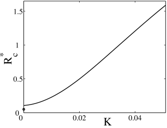
Figure 6: Convection threshold $R_{c}^{*}$ versus the Knudsen number $K$ at $F=0.1$. As $K\to 0$, the value of $R_{c}^{*}$ is greater than the Schwarzschild’s value $R_{S}(F=0.1)\simeq 0.05$, shown by the empty circle.

IV Summary

We performed a linear stability analysis of the static state in a horizontal layer of granular gas driven from below. The hydrodynamic theory Meerson that we employed in our analysis is expected to be valid when the mean free path of the particles is much smaller than any length scale described hydrodynamically. We have found the convection threshold, in terms of the relative heat loss number $R$, versus the two other scaled numbers of the problem: the Froude number $F$ and the Knudsen number $K$. We have predicted the morphology of convection cells at the onset of convection. As $F\to 0$, the convection instability goes over continuously into the phase-separation instability Livne ; Brey ; Khain ; Livne2 ; Argentina ; MPSS . At large $F$ the convection threshold depends only on $K$. We established a simple connection between thermal granular convection and classical thermal convection of ideal compressible fluid. The connection is given in terms of the Schwarzschild’s criterion, a universal necessary (but not sufficient) condition for thermal convection. A further development of the theory should account for the excluded-volume effects Jenkins . Importantly, the simple Schwarzschild’s criterion will be readily available in the finite-density theory. Indeed, this criterion requires only the knowledge of the static profiles of the granular temperature and density and the constitutive relation for the granular entropy.

V Acknowledgments

We gratefully acknowledge useful discussions with Igor S. Aranson, John M. Finn, Xiaoyi He, Pavel V. Sasorov and Victor Steinberg. The work was supported by the Israel Science Foundation administered by the Israel Academy of Sciences and Humanities.

References

- (1) G.H. Ristow, Pattern Formation in Granular Materials, (Springer, Berlin, 2000).
- (2) R. Ramìrez, D. Risso, and P. Cordero, Phys. Rev. Lett. 85, 1230 (2000).
- (3) R.D. Wildman, J.M. Huntley, and D.J. Parker, Phys. Rev. Lett. 86, 3304 (2001).
- (4) P. Sunthar and V. Kumaran, Phys. Rev. E 64, 041303, (2001).
- (5) X. He, B. Meerson, and G. Doolen, Phys. Rev. E 65, 030301(R) (2002).
- (6) J. Talbot and P. Viot, Phys. Rev. Lett. 89, 064301; 179904 (2002).
- (7) S. Chandrasekhar, Hydrodynamic and Hydromagnetic Stability (Dover, New York, 1981).
- (8) L.D. Landau and E.M. Lifshitz, Course of Theoretical Physics: Vol. 6 Fluid Mechanics (Pergamon, Oxford, 1987), pp. 7-8.
- (9) E.A. Spiegel, Astrophys. J. 141, 1068 (1965).
- (10) M.S. Gitterman and V.A. Steinberg, High Temp. 8, 754 (1970); J. Appl. Math. Mech. 34, 305 (1971).
- (11) M. Gitterman, Rev. Mod. Phys. 50, 85 (1978).
- (12) P. Carlès and B. Ugurtas, Physica D 126, 69 (1999).
- (13) J.T. Jenkins and M.W. Richman, Phys. Fluids 28, 3485 (1985).
- (14) J.J. Brey, J.W. Dufty, C.S. Kim, and A. Santos, Phys. Rev. E 58, 4638 (1998).
- (15) S.E. Esipov and T. Pöschel, J. Stat. Phys. 86, 1385 (1997); E.L. Grossman, T. Zhou, and E. Ben-Naim, Phys. Rev. E 55, 4200 (1997); J.J. Brey and D. Cubero, in Granular Gases, edited by T. Pöschel and S. Luding (Springer, Berlin, 2001), pp. 59-78; I. Goldhirsch, ibid, pp. 79-99.
- (16) M.C. Cross and P.C. Hohenberg, Rev. Mod. Phys. 65, 851 (1993); E. Bodenschatz, W. Pesch and G. Ahlers, Annu. Rev. Fluid. Mech. 32, 709 (2000).
- (17) E. Livne, B. Meerson, and P.V. Sasorov, cond-mat/008301; Phys. Rev. E 65, 021302 (2002).
- (18) J.J. Brey, M.J. Ruiz-Montero, F. Moreno, and R. García-Rojo, Phys. Rev. E 65, 061302 (2002).
- (19) E. Khain and B. Meerson, Phys. Rev. E 66, 021306 (2002); cond-mat/0201569.
- (20) E. Livne, B. Meerson, and P.V. Sasorov, Phys. Rev. E 66, 0503XX (2002); cond-mat/0204266.
- (21) M. Argentina, M.G. Clerc, and R. Soto, Phys. Rev. Lett. 89, 044301 (2002).
- (22) B. Meerson, T. Pöschel, P.V. Sasorov, and T. Schwager, cond-mat/0208286.
- (23) Our results, obtained with the high-precision linear solver, are in qualitative agreement with the results of lattice-Boltzmann (LB) simulation in a square box (that is, for ) reported in Ref. Meerson . There is, however, a systematic quantitative disagreement (by a factor of ) in the value of obtained with the two methods for , and and . The LB scheme LB was originally developed and tested for nearly incompressible fluid. The observed disagreement indicates that the LB scheme becomes inaccurate at moderate density/temperature contrasts intrinsic in this granular system. We are grateful to Xiaoyi He for a useful discussion of this issue.
- (24) X. He, S.Y. Chen, and G.D. Doolen, J. Comput. Phys. 146, 282 (1998).