Quantum Hall Skyrmions in the framework of O(4) Non-linear Sigma Model

Abstract

A new framework for quantum Hall skyrmions in $O(4)$ nonlinear sigma model is studied here. The size and energy of the skyrmions are determined incorporating the quartic stability term in the Lagrangian. Moreover, the introduction of a $\theta$-term determines the spin and statistics of these skyrmions.

I Introduction

Skyrmions are generally described by nonlinear sigma model. A smooth texturing of the spins can be described by an effective nonlinear sigma model where the spin is described as a unit vector ${\bf{n}}({\bf{r}})$. This spin vector ${\bf{n}}$ lies on a sphere $S^{2}$ where we may consider a magnetic monopole located at the centre. Skyrmions are characterized by the topological charge $Z=\int d{\bf{r}}q({\bf{r}})$ where $q={\bf{n}}.(\partial_{x}{\bf{n}}\times\partial_{y}{\bf{n}})/4\pi$ is the Pontryagin density. Z is the winding number of the mapping ${\bf{n}}({\bf{r}})$ from the compactified space $S^{2}$ to the target space of the sigma model $(S^{2})$ and is given by the homotopy $\pi_{2}(S^{2})=Z$. The topological density is proportional to the deviation of the electron density from its uniform value $\rho_{0}$.

In analogy to the Ginzburg-Landau description of superconductivity, the Chern-Simons theory of quantum Hall systems was derived by Zhang, Hansson and Kivelson 5 which was subsequently extended by Lee and Kane 6 to describe the spin unpolarized quantum Hall liquid. In a quantum Hall fluid, the ground state has been found to be a fully spin polarized quantum ferromagnet. By noticing that the dynamics of quantum Hall system with a spin polarized ground state will follow that of a quantum ferromagnet and that the skyrmion is a charged object of the system, Sondhi et.al. s1 ; s2 proposed a phenomenological action which is valid for the long wave length and small frequency limit. In this scheme, the competition between the Zeeman and Coulomb terms sets the size and energy of the skyrmions and modifies the detailed form of their profiles. In case the Zeeman energy and Coulomb energy are taken to be vanishing, analytic expressions are available for the skyrmions and their energy is independent of their size. This scale invariance is broken by the Zeeman and Coulomb terms in the Lagrangian.

To study low energy excitations for partially polarized states a nonlinear $\sigma$-model has been developed 7 considering a two component quantum Hall system within a Landau-Ginzberg theory with two Chern-Simons gauge fields. It has been found that these excitations have finite energy due to the presence of the Chern-Simons gauge field and closely resemble the skyrmions in the usual nonlinear $\sigma$-model. Skyrmions in arbitrary polarized quantum Hall states are studied ssm employing a doublet model taking into account two fields carrying the spin index in Chern-Simons term with a matrix valued coupling strength.

Skyrmion excitations in quantum Hall systems at $\nu=1$, using finite size calculations xh , is studied in spherical geometry where electrons reside on the surface of a sphere with a monopole at the centre. For a monopole of total magnetic flux $N_{\phi}=2\mu$ the lowest Landau level degeneracy is $2\mu+1$. All single particle states in lowest Landau level have fixed angular momentum value $\mu$. At filling factor $\nu=1$ corresponding to the electron number $N=2\mu+1$ the ground state is spin polarized independent of the strength of the Zeeman splitting. When an additional flux is added or removed from the system, the ground state is a skyrmion (antiskyrmion) with topological charge $Q=+1(-1)$. The energy gap is determined by the interplay of the Zeeman energy and electron-electron interaction.

In this note, we shall study the static properties of skyrmions in spherical geometry considering a $O(4)$ nonlinear $\sigma$-model in $3+1$ dimensional manifold. In some earlier papers rev11 ; bb we have analyzed the hierarchy of quantum Hall states in spherical geometry from the view point of chiral anomaly and Berry phase. In this framework it is shown that the Magnus force acting on vortices and skyrmions in the quantum Hall system is generated by the background field associated with the chirality of the system bdm . The various polarization states of quantum Hall fluid is also studied and their low energy excitations are examined using a homotopic analysis bdp . The $O(4)$ nonlinear $\sigma$-model helps us to have two independent subalgebras each isomorphic to a $SU(2)$ algebra so that the left and right group can be taken to be associated with two mutually opposite orientations of the magnetization vector which resides on the $2D$ surface of the sphere. The homotopic analysis then suggests that for fully polarized states the low energy excitations are skyrmions. It is here shown that the addition of the quartic stability term introduced by Skyrme, known as the Skyrme term in the literature, will determine the size of the quantum Hall skyrmions in this framework. This also helps us to determine the spin and statistics of the skyrmion through the introduction of the topological $\theta$-term in the Lagrangian.

In sec.2 we recapitulate the study of skyrmion excitations in quantum Hall fluid when the system is described by means of the Zhang-Hansson-Kivelson model and modified by Lee and Kane to take into account the effect of spin. In sec.3 we shall describe quantum Hall skyrmions in spherical geometry considering a $O(4)$ nonlinear $\sigma$-model taking into account the Skyrme term and $\theta$-term. In sec.4 we shall determine the size and energy of the skyrmion in this formalism.

II Quantum Hall Skyrmions in Planar Geometry

We here recapitulate the works on quantum Hall skyrmions on the basis of the bosonic theory of an electron which is viewed as a composite object of a boson and a flux tube carrying an odd multiple of flux quanta $\Phi_{0}=h/e$ attached via a Chern-Simons term. We begin with the Landau-Ginzburg theory of the Hall effect introduced by Zhang, Hansson and Kivelson 5 and modified by Lee and Kane 6 to incorporate the effect of the spin. We consider the Lagrangian st

$$L= i\phi^{\dagger}[\partial_{0}-i(a_{0}+eA_{0})]\phi$$ (1)

$$-\frac{1}{2m^{*}}|[\partial_{i}-i(a_{i}+eA_{i})]\phi|^{2}$$

$$-\frac{\lambda}{2}(|\phi|^{2}-\rho_{0})^{2}+\frac{1}{4\theta}\epsilon^{\mu\nu\sigma}a_{\mu}\partial_{\nu}a_{\sigma}$$

Here $\phi=(\phi_{1},\phi_{2})$ is a two component complex scalar field. $\theta$ is the statistics parameter which takes the values $\theta=(2n+1)\pi$ so that the boson field $\phi$ represents a fermion, $A_{\mu}$ the external electromagnetic field and $m^{*}$ is the effective mass of the electron. To determine the size and energy of the skyrmions Zeeman and Coulomb interactions should be included. However, to study the topological features we can ignore them for the moment. We consider a solution with uniform density $\rho=(|\phi_{1}|^{2}+|\phi_{2}|^{2})=\rho_{0}$ at filling fraction $\nu=\frac{1}{2n+1}$. In order to separate the amplitude and spin degrees of freedom we introduce the CP¹ field $\bf{z}$ and we write

$$\phi=\sqrt{\rho}\bf{z}$$ (2)

The Lagrangian (1) now takes the form

$$L= i\rho{\bf{z}}^{{\dagger}}[\partial_{0}-i(a_{0}+eA_{0})]{\bf{z}}$$ (3)

$$-\frac{\rho}{2m^{*}}|[\partial_{i}-i(a_{i}+eA_{i})]{\bf{z}}|^{2}$$

$$-\frac{\lambda}{2}(\rho-\rho_{0})^{2}+\frac{1}{4\theta}\epsilon^{\mu\nu\sigma}a_{\mu}\partial_{\nu}a_{\sigma}$$

Here $\bf{z}$ is a two component complex field with the constraint ${\bf{z}}^{{\dagger}}{\bf{z}}=|z_{1}|^{2}+|z_{2}|^{2}=1$.

One can now use the identity

$$\frac{\rho}{2m^{*}}|[\partial_{i}-i(a_{i}+eA_{i})]{\bf{z}}|^{2}=\frac{\rho}{8m^{*}}(\bigtriangledown{\bf{n}})^{2}+\frac{m^{*}}{2\rho}\bf{J}^{2}$$ (4)

where ${\bf{J}}=(J^{1},J^{2})$ with

$$J^{i}=\frac{\rho}{m^{*}i}[{\bf{z}}^{{\dagger}}\partial_{i}{\bf{z}}-i(a_{i}+eA_{i})]$$ (5)

The local spin direction is given by

$$n^{a}={\bf{z}}^{{\dagger}}\sigma^{a}{\bf{z}}$$ (6)

and $\nabla{\bf{n}}=(\partial_{1}{\bf{n}},\partial_{2}{\bf{n}})$. The term $\frac{\rho}{8m*}(\nabla{\bf{n}})^{2}$ corresponds to the static nonlinear sigma model.

Now introducing Hubbard-Stratanovich transformation ${\bf{J}}$ with the relation $J_{0}=\rho$ so that the current 3-vector $(J^{0},J^{1},J^{2})$ is promoted to the status of an independent dynamical variable, the Lagrangian can be written as

$$\begin{array}[]{lcl}L&=&\displaystyle{i\rho[{\bf{z}}^{{\dagger}}\partial_{0}{\bf{z}}-i(a_{0}+eA_{0})]}\\ &&\displaystyle{+i[{\bf{z}}^{{\dagger}}\partial_{i}{\bf{z}}-i(a_{i}+eA_{i})]J^{i}+\frac{m^{*}}{2\rho}{\bf{J}}^{2}}\\ &&\displaystyle{-\frac{\rho}{8m*}(\nabla{\bf{n}})^{2}-\frac{\lambda}{2}(\rho-\rho_{0})^{2}+\frac{1}{4\theta}\epsilon^{\mu\nu\lambda}a_{\mu}\partial_{\nu}a_{\lambda}}\\ \end{array}$$ (7)

Integrating over the $U(1)$ phase degree of freedom in ${\bf z}$ we arrive at the current conservation law $\partial_{\alpha}J_{\alpha}=0$ and we have current 3-vector $(\rho=J^{0},J^{1},J^{2})$ as the curl of a three dimensional vector field. One can set $J^{\mu}_{[0]}=(\rho_{0},0,0)$ equal to $\epsilon^{\mu\nu\sigma}\partial_{\nu}{\cal{A}}^{[0]}_{\sigma}$ and

$$J^{\mu}-J^{\mu}_{[0]}=\epsilon^{\mu\nu\sigma}\partial_{\nu}\mathcal{A}_{\sigma}$$ (8)

Integrating out the Chern-Simons field $a_{\mu}$ and using the relation $2\theta\rho_{0}=eB_{z}$, we can finally arrive at the relation

$$\begin{array}[]{lcl}L&=&\displaystyle{2\pi{\cal{J}}^{\mu}_{S}({\cal{A}}_{\mu}+{\cal{A}}^{[0]}_{\mu})-\theta{J^{\mu}}{\cal{A}}_{\mu}}\\ &&\displaystyle{+\frac{m^{\ast}}{2\rho}{\bf{J}}^{2}-\frac{\rho}{8m^{\ast}}(\nabla{\bf{n}})^{2}-\frac{\lambda}{2}(J^{0}-J^{0}_{[0]})^{2}}\\ \end{array}$$ (9)

where

$${\mathcal{J}}^{\mu}_{S}={\frac{1}{2{\pi}i}}\epsilon^{\mu\nu\sigma}\partial_{\mu}\bar{z}_{\sigma}\partial_{\nu}z_{\sigma}$$ (10)

is the skyrmion number current.

Defining the field strength term  $\cal{F}_{\mu\nu}=\partial_{\mu}\cal{A}_{\nu}-\partial_{\nu}\cal{A}_{\mu}$  to be the dual of the electron number current and adjusting the unit of length and time such that $c=\sqrt{\lambda\rho_{0}/m^{*}}$, the velocity of density waves in the absence of magnetic field becomes unity, we can write

$$\begin{array}[]{lcl}L&=&\displaystyle{2\pi{\cal{J}}^{\mu}_{S}({\cal{A}}_{\mu}+{\cal{A}}^{[0]}_{\mu})-\frac{1}{2}\theta\epsilon^{\mu\nu\sigma}{\cal{A}}_{\mu}{\cal{F}}_{\nu\sigma}}\\ &&\displaystyle{-\frac{\lambda}{4}{\cal{F}}_{\mu\nu}{\cal{F}}^{\mu\nu}-\frac{1}{8\lambda}(\nabla{\bf{n}})^{2}}\\ \end{array}$$ (11)

It is noted that the skyrmion number current acts as a source for a topologically massive gauge field ${\mathcal{A}}_{\mu}$ st and also sees the background field ${\mathcal{A}}^{[0]}_{\mu}$.

Incorporating Zeeman and Coulomb terms Sondhi et.al. s1 considered the following modified form of the Lagrangian (1).

$$\begin{array}[]{lcl}L({\bf{r}})&=&\displaystyle{\phi^{{\dagger}}({\bf{r}})[\partial_{0}-i(a_{0}+eA_{0})]\phi({\bf{r}})]}\\ &&\displaystyle{-\frac{1}{2m^{*}}|[\partial_{i}-i(a_{i}+eA_{i})]\phi({\bf r})|^{2}}\\ &&\displaystyle{-\frac{1}{2}\int d^{2}r^{\prime}V({\bf{r}}-{\bf{r}}^{\prime})[|\phi({\bf{r}})|^{2}-\rho_{0}][|\phi({\bf{r}}^{\prime})|^{2}-\rho_{0}]}\\ &&\displaystyle{-\frac{e^{2}}{4\theta}\epsilon^{\mu\nu\sigma}a_{\mu}({\bf{r}})\partial_{\nu}a_{\sigma}({\bf{r}})-\frac{1}{2}g\mu_{B}B\phi^{{\dagger}}({\bf{r}})\sigma^{z}\phi({\bf{r}})}\\ \end{array}$$ (12)

Here $V=e^{2}/\epsilon r$ is the interparticle Coulomb potential and $\mu_{B}$ is the Bohr magneton.

Noting that $\phi_{\alpha}=\sqrt{\rho}z_{\alpha}$ where $\sum{z_{\alpha}}^{{\dagger}}z_{\alpha}=1$ and using the mapping $n^{a}={\bf{z}}^{{\dagger}}\sigma^{a}{\bf{z}}$, we can replace the CP¹ field by an $O(3)$ sigma model field. Indeed, by observing that at the ground state the dynamics of the system is that of a ferromagnet with a long range interaction arising from the Coulomb interaction between the underlying electrons, we take into account the necessary terms and consider the Lagrangian st

$$\begin{array}[]{lcl}L_{eff}&=&\displaystyle{\frac{1}{2}\rho^{0}{\bf{A}}({\bf{n}}).\partial_{t}{\bf{n}}-\frac{1}{2}\rho^{s}(\nabla{\bf{n}})^{2}}\\ &&\displaystyle{+\frac{1}{2}g\rho_{0}\mu_{B}{\bf{n}}.{\bf{B}}-\frac{e^{2}}{2\epsilon}\int d^{2}r^{\prime}\frac{q({\bf{r}})q({\bf{r}}^{\prime})}{|{\bf{r}}-{\bf{r}}^{\prime}|}}\\ \end{array}$$ (13)

Here $\bf{A}$ is the vector potential of a unit magnetic monopole, $\rho^{s}$ is the spin stiffness ($\rho^{s}={e^{2}}/{16\sqrt{2\pi}\epsilon l}$ for $\nu=1$), $\epsilon$ is the dielectric constant and $l$ is the magnetic length. $q({\bf{r}})={\bf{n}}.(\partial_{x}{\bf{n}}\times\partial_{y}{\bf{n}})/4\pi$ is the topological density. This topological density is proportional to the deviation of the electron density $\rho$ from its uniform value; $q=\nu(\rho-\rho_{0})$. The topological charge is $Z=\int d{\bf{r}}q({\bf{r}})$. For $\nu=1$, skyrmions with topological charge $Z$ carry electric charge $-Z|e|$.

The Zeeman and Coulomb terms break the scale invariance. Their profiles now depend on the dimensionless ratio $\tilde{g}=(g\mu_{B}B)/(e^{2}/\epsilon l^{2})$ of the Zeeman energy to Coulomb energy. For $Z=1$ skyrmions the scale invariant solution yields a Zeeman energy that diverges logarithmically with system size for any $\lambda$. This can be fixed by matching the scale invariant solution onto the exact asymptotic solution in the outer region. This suggest for $Z=1$ the size s3

$${\lambda}=0.558~{}l(\tilde{g}|\ln\tilde{g}|)^{-1/3}$$ (14)

and energy

$$E=\frac{e^{2}}{\epsilon l}~{}[\sqrt{\frac{\pi}{32}}+0.622~{}(\tilde{g}|\ln\tilde{g}|)^{1/3}]$$ (15)

Indeed at large $g$ the quasiparticles are single particle-like and may carry charge and spin $S_{z}=1/2$ and have size $l$. At small $g$, they still carry charge $\pm e$ but diverge in size and have nontrivial spin with a divergent $z$-component of spin $S_{z}$ (the number of reversed spin) as well as divergent total spin.

III Quantum Hall Skyrmions in $3+1$ dimensional manifold

We want to study the low energy topological excitations of the quantum Hall fluid within the framework of $O(4)$ nonlinear $\sigma$-model in $3+1$ dimensional manifold. In this geometry, electrons are placed on the surface of a sphere under the influence of an uniform radial magnetic field. The magnetic field is produced by a magnetic monopole of strength $\mu$ placed at the centre of the sphere. As we know, the angular momentum in the field of a magnetic monopole is given by

$${\bf{J}}={\bf{r}}\times{\bf{p}}-\mu{\bf{\hat{r}}}$$ (16)

where $\mu$ can take the values $0,\pm 1/2,\pm 1,\pm 3/2,........$. Evidently, eigenvalues of ${\bf J}$ can take the values $|\mu|$, $|\mu|+1$, $|\mu|+2$,……. In this geometry the quantum Hall states can be depicted by a two-component spinor $\left(\begin{array}[]{c}u\\ v\end{array}\right)$ such that $u~{}=~{}\cos{\theta/2}~{}e^{i\phi/2}$ and $v~{}=~{}\sin{\theta/2}~{}e^{-i\phi/2}$ b1 and

$$|\psi_{\nu=1}\rangle~{}=~{}\prod_{i,j}~{}(u_{i}v_{j}-v_{i}u_{j})$$ (17)

is the spin polarized ground state at $\nu=1$.

The generalized state for $\nu=1/m$, $m$ being an odd integer, is written as rev11 ; h1

$$|\psi_{\nu}\rangle~{}=~{}\prod_{i<j}~{}(u_{i}v_{j}-v_{i}u_{j})^{1/{\nu}}$$ (18)

However it should be added that at $\nu=1$ we have a non-interacting spectrum which is never a correspondence for $\nu=1/m$, with $m$ being an odd integer. Indeed FQH states correspond to interacting systems.

The skyrmion state can be written as

$$|\psi\rangle~{}=~{}C^{\prime}\prod_{k}\left(\begin{array}[]{c}v_{k}\\ -\alpha u_{k}\end{array}\right)|\psi_{\nu}\rangle$$ (19)

where the spin texture is included within the components $v_{k}$ and $u_{k}$ and $0\leq\alpha\leq 1$.

Actually, if a smooth and monotonical function $g(\theta)$ is defined with $g(0)=0$ and $g(\pi)=\pi$ then the skyrmion state can be written as xh

$$\hat{\phi}(\Omega)~{}=~{}\cos(g(\theta)-\theta)~{}\hat{e_{r}}+~{}\sin(g(\theta)-\theta)~{}\hat{e_{\theta}}$$ (20)

where $\hat{e_{r}}$ and $\hat{e_{\theta}}$ are the basis vectors. The size of a skyrmion is determined by the function $g(\theta)$ and $g(\theta)=\theta$ describes the hedgehog skyrmion with spin in the radial direction $\hat{r}$.

This is the skyrmion state with the constraint $|\hat{\phi}(\Omega)|=1$.

The quantum state for the classical skyrmion $\hat{\phi}(\Omega)$ can be written as

$$|\psi\rangle=~{}C.P\prod_{k}\left(\begin{array}[]{c}\sin{g(\theta_{k})/2}~{}~{}e^{-i\phi_{k}/2}\\ -\cos{g(\theta_{k})/2}~{}~{}e^{i\phi_{k}/2}\end{array}\right)|\psi_{\nu}\rangle$$ (21)

where $C$ is the normalization constant, $P$ is the projection operator to the lowest Landau level and $g(\theta)$ controls the size of the skyrmion xh . From eqns. (19) and (21) it is seen that $0\leq\alpha\leq 1$ is determined from $g(\theta)$ and it controls the size of the skyrmion.

The size of the skyrmion can be defined by the position where spin direction is perpendicular to the radial (and spin) direction at either pole. With this convention, the skyrmion size is

$$\theta_{0}=2arc\tan\alpha$$ (22)

which equals $\pi/2$ for the hedgehog skyrmion with $\alpha=1$

Bychkov et. al. have shown by that the quantum Hall skyrmions consist of a core whose size is defined by the interplay between the Zeeman and Coulomb energies and an additional length scale $l_{sk}$ which determines the tail of the spin distribution. This characteristic length is given by

$${l_{sk}}^{-2}=2\sqrt{2/{\pi}}|\tilde{g}|(a_{B}/l^{3})$$ (23)

where $\tilde{g}$ is the effective $g$ factor, $a_{B}=\epsilon\hbar^{2}/me^{2}$ is the Bohr radius, $\epsilon$ being the dielectric constant and $l$ is the magnetic length. It is noted that as $\tilde{g}\rightarrow 0$, $l_{sk}\rightarrow\infty$, we can take

$$\cot{\theta/2}=x/x_{0}$$ (24)

where $x$ and $x_{0}$ are two dimensionless parameters given by $x=r/l_{sk}$ and $R=x_{0}l_{sk}$, $R$ being the size of the skyrmion core region.

We can associate $\alpha$ with $x_{0}/x$ where $x_{0}\ll 1$ and $x\ll 1$ i.e. for $r$ far away from the exponential tail of the skyrmion. It is pointed out that in the region $x_{0}\ll x\ll 1$, $r$ is far outside the skyrmion core.

In the framework of $O(4)$ nonlinear $\sigma$-model the size of the skyrmion is determined by the quartic stability term, known as the Skyrme term. Indeed, taking the spin variable ${\bf{z}}=U{\bf{z_{0}}}$ where ${\bf{z}}_{0}=\left(\begin{array}[]{c}1\\ 0\end{array}\right)$ and $U\in SU(2)$, we may write the nonlinear sigma model Lagrangian in terms of the $SU(2)$ matrices $U$ as sk

$$L=~{}-\frac{M^{2}}{16}~{}(\partial_{\mu}U^{{\dagger}}\partial_{\nu}U)-\frac{1}{32\eta^{2}}~{}[\partial_{\mu}UU^{{\dagger}},\partial_{\nu}UU^{{\dagger}}]^{2}$$ (25)

where $M$ is a constant of dimension of mass and $\eta$ is a dimensionless coupling parameter. The $\alpha$ dependence may be incorporated through $M$ and $\eta$ where these parameters are taken as functions of $\alpha$.

To have a geometrical interpretation of the Skyrme term (eqn.(25)), we note that it effectively corresponds to the vorticity of the system which prevents it from shrinking it to zero size. In fact in an axisymmetric system where the anisotropy is introduced along a particular direction through the introduction of a magnetic monopole at the centre, the components of the linear momentum satisfy a commutation relation of the form

$$[p_{i},p_{j}]=i\mu~{}\epsilon_{ijk}~{}\frac{x^{k}}{r^{3}}$$ (26)

When the position space is a 3-sphere $S^{3}$ with a monopole at the centre, we can have a commutation relation of the form

$$[p_{i},p_{j}]=\frac{i}{R}~{}\epsilon_{ijk}~{}p_{k}$$ (27)

where R is proportional to the radius of the $S^{3}$. For a distorted sphere we can consider $R$ as a functional form $R(\theta,\phi)$ corresponding to the core radius of the skyrmion. We can define the core size of the skyrmion such that $R=R_{0}(1-\alpha)$ where $R_{0}$ is the size of the skyrmion having minimal energy.

In view of this, in $3+1$ dimensions we can generalize the Lagrangian (11) incorporating the Skyrme term in the form

$$\begin{array}[]{lcl}L{}&=&\displaystyle{~{}2\pi\tilde{{\cal{J}}}^{S}_{\mu}~{}({\cal{A}}_{\mu}+{\cal{A}}^{[0]}_{\mu})-~{}\frac{M^{2}}{16}~{}Tr(\partial_{\mu}U^{{\dagger}}\partial_{\nu}U)-\frac{1}{32\eta^{2}}~{}Tr[\partial_{\mu}UU^{{\dagger}},\partial_{\nu}UU^{{\dagger}}]^{2}}\\ &&\displaystyle{-\frac{\theta}{16\pi^{2}}~{}{{}^{*}{\mathcal{F}}_{\mu\nu}}{\mathcal{F}}_{\mu\nu}-\frac{1}{4}{\mathcal{F}}_{\mu\nu}{\mathcal{F}}^{\mu\nu}}\\ \end{array}$$ (28)

Here $\theta=g/c^{2}$ with $g=\nu e^{2}/h$ as Hall conductivity and $~{}^{*}{\mathcal{F}}_{\mu\nu}$ is a Hodge dual given by

$${}^{*}{\mathcal{F}}_{\mu\nu}=\frac{1}{2}~{}\epsilon_{\mu\nu\lambda\sigma}{\mathcal{F}}_{\lambda\sigma}$$ (29)

This is associated with $O(4)$ nonlinear sigma model where the topological current is defined as

$$\tilde{{\mathcal{J}}}^{S}_{\mu}~{}=~{}\frac{1}{24\pi^{2}}~{}\epsilon_{\mu\nu\alpha\beta}Tr(U^{-1}\partial_{\nu}U)(U^{-1}\partial_{\alpha}U)(U^{-1}\partial_{\beta}U)$$ (30)

and ${\cal{A}}_{\mu}[{\cal{A}}^{[0]}_{\mu}]$ is a four vector. It is to be mentioned that we have taken the kinematic term (second term in equation (28)) which takes into account spin waves, the Goldstone modes associated with a ferromagnetic ground state. The $SU(2)$ matrix $U$ is here defined as

$$U=n_{0}I+\bf{n}.\overrightarrow{\tau}$$ (31)

where the chiral fields $n_{0}$,$n_{1}$,$n_{2}$ and $n_{3}$ satisfy the relation $\sum n_{i}^{2}=1$.

It may be noted that in $2+1$ dimension, we have the normalized $3$-vector field ${\bf n}$ with $\sum n^{2}_{i}=1$ where $n_{i}$ corresponds to the local spin direction. In the $O(4)$ model $n_{i}(i=1,2,3)$ corresponds to this spin direction which live on the $2$-dimensional surface of the sphere where the extra field $n_{0}$ helps us to consider three ”boost” generators in $(n_{0},n_{i})$ planes. In view of this, we can consider two types of generators such that the generator $M_{k}$ rotates the $3$-vector $\bf{n}(x)$ to any chosen axis and the boost generators $N_{k}$ would mix $n_{0}$ with the components of $\bf{n}$. We can now construct the following algebra

$$[M_{i},M_{j}]={i\epsilon_{ijk}M_{k}}$$

$$[M_{i},N_{j}]={i\epsilon_{ijk}N_{k}}$$

$$[N_{i},N_{j}]={i\epsilon_{ijk}M_{k}}$$ (32)

which is locally isomorphic to the Lie algebra of the $O(4)$ group. This helps us to introduce the left and right generators

$$L_{i}=\frac{1}{2}(M_{i}-N_{i})$$

$$R_{i}=\frac{1}{2}(M_{i}+N_{i})$$ (33)

which satisfy

$$[L_{i},L_{j}]={i\epsilon_{ijk}L_{k}}$$

$$[R_{i},R_{j}]={i\epsilon_{ijk}R_{k}}$$

$$[L_{i},R_{j}]=0$$ (34)

Thus the algebra has split into two independent subalgebras each isomorphic to a $SU(2)$ algebra and corresponds to the chiral group $SU(2)_{L}\otimes SU(2)_{R}$. The left and right chiral group can now be taken to be associated with two mutually opposite orientations of the magnetization vector which resides on the $2$D surface of the sphere.

It may be mentioned that the $P$ and $T$ violating $\theta$-term $(-\frac{\theta}{16\pi^{2}}~{}{{}^{*}{\mathcal{F}}_{\mu\nu}}{\mathcal{F}}_{\mu\nu})$ in $3+1$ dimensions corresponds to the Chern-Simons term in $2+1$ dimension. This term is related to chiral anomaly and we have the Pontryagin index given by db

$$q~{}=~{}2\mu=~{}-{\frac{1}{16\pi^{2}}}~{}\int Tr^{*}{\mathcal{F}}_{\mu\nu}{\mathcal{F}}_{\mu\nu}d^{4}x$$ (35)

It may noted that in $2+1$ dimensions, the topological current

$$J_{\mu}=\frac{1}{8\pi}~{}\epsilon_{\mu\nu\lambda}{\bf{n}}.(\partial_{\nu}{\bf{n}}\times\partial_{\lambda}{\bf{n}})$$ (36)

may be related to the gauge field current

$$J_{\mu}=\epsilon_{\mu\nu\lambda}\nabla_{\nu}{\cal{A}}_{\lambda}$$ (37)

which helps us to write the Chern-Simons term as

$$W=\frac{\theta}{4\pi}\int d^{3}x\epsilon_{\mu\nu\lambda}{\cal{A}}_{\mu}\nabla_{\nu}{\cal{A}}_{\lambda}$$ (38)

Evidently this relates to the Hopf invariant which can be explicitly written in terms of $SU(2)$ matrix $U(x)$ which rotates the vector ${\bf n}$ to the chosen (third) axis ${\bf n}.{\vec{\tau}}=U^{-1}\tau_{3}U$ and the Hopf invariant is given by

$$H=\frac{\epsilon_{\mu\nu\lambda}}{24\pi^{2}}\int d^{3}xTr(U^{-1}\partial_{\mu}U)(U^{-1}\partial_{\nu}U)(U^{-1}\partial_{\lambda}U)$$ (39)

which is a degree of mapping of the (2+1) dimensional space time into $SU(2)$ and is given by the homotopy $\pi_{3}(S^{3})=Z$. In $3+1$ dimensions, if we consider Euclidean four dimensional space-time such that ${\mathcal{F}}_{\mu\nu}=0$ at all points on the boundary $S^{3}$ of a certain volume $V^{4}$ inside which ${\mathcal{F}}_{\mu\nu}\neq 0$ then the gauge potential tends to be a pure gauge in the limiting case towards the boundary i.e. we have

$${\cal{A}}_{\mu}=U^{-1}\partial_{\mu}U,~{}~{}~{}~{}~{}~{}~{}~{}~{}~{}~{}~{}~{}~{}U\in SU(2)$$ (40)

This then helps us to write the topological charge of quantum Hall skyrmions given by eqn.(38) as the winding number

$$Z~{}=~{}{\frac{1}{24\pi^{2}}}~{}\int_{S^{3}}dS_{\mu}~{}\epsilon^{\mu\nu\lambda\sigma}[(U^{-1}\partial_{\nu}U)(U^{-1}\partial_{\lambda}U)(U^{-1}\partial_{\sigma}U)]$$ (41)

which is given by the homotopy $\pi_{3}(S^{3})=Z$ and the electric charge is given by $\nu eZ$. We observe here that the Pontryagin index given by $q=2\mu$ in eqn.(35) introduces the Berry phase for quantum Hall states as $\mu$ represents magnetic monopole strength. Indeed, the flux through the sphere is $2\mu$ and the phase is given by $e^{i\phi_{B}}$ where $\phi_{B}=2\pi\nu$ (number of flux quanta enclosed by the loop). When a $Z=1$ skyrmion is moved around a closed loop it acquires a Berry phase $2\pi\nu N$ where $N$ is the number of skyrmions enclosed by the loop. To find the spin and statistics, we consider a process which exchanges two skyrmions in the rest frame of one of the skyrmions. This exchange effectively corresponds to the other skyrmion moving around the first in a half circle and hence it picks up a phase $\pi~{}\nu$ which is the statistical phase of a skyrmion. For $\nu=1$ it is a fermion and $\nu=1/m$, $m$ being an odd integer it corresponds to an anyon in planar geometry. In general, the spin of the skyrmion having charge $\nu eZ$ is given by $\nu Z/2$.

IV Skyrmion Size and Energy

From our above discussions, we now observe that the energy of a free skyrmion depends on the following two terms in the Lagrangian (28)

$$L=-~{}\frac{M^{2}}{16}~{}(\partial_{\mu}U^{{\dagger}}\partial_{\nu}U)-\frac{1}{32\eta^{2}}~{}[\partial_{\mu}UU^{{\dagger}},\partial_{\nu}UU^{{\dagger}}]^{2}$$ (42)

The static nonlinear sigma model Lagrangian corresponding to eqn. (42) gives rise to the energy integral as

$$E=\int d^{3}x\{\frac{M^{2}}{16}Tr(\nabla U^{{\dagger}}\nabla U)+\frac{1}{32\eta^{2}}Tr[\partial_{i}UU^{{\dagger}},\partial_{j}UU^{{\dagger}}]^{2}\}$$ (43)

where $(i,j=1,2,3)$

To compute the energy, we take the Skyrme ansatz sk

$$U(x)=exp~{}[iF(r)\overrightarrow{\tau}.{\bf{\hat{x}}}]$$ (44)

where $\overrightarrow{\tau}$ are Pauli matrices, $\bf{\hat{x}}=\frac{x_{i}}{r}$ and $F(0)=\pi$ and $F(r)\rightarrow 0$ as $r\rightarrow\infty$; $r$ is the spherical radius in $3$-dimensional manifold. We explicitly write $U=\cos{F(r)}+i\overrightarrow{\tau}.{\bf{\hat{x}}}\sin{F(r)}$ with $\cos{F(r)}=\frac{1-(r/R)^{2}}{1+(r/R)^{2}}$,   $\sin{F(r)}=\frac{2(r/R)}{1+(r/R)^{2}}$. The energy integral becomes

$$E(R)=4\pi^{2}M^{2}R~{}I_{1}+~{}2\pi^{2}\frac{I_{2}}{\eta^{2}R}$$ (45)

where

$$I_{1}=\frac{1}{\pi}\int^{\infty}_{0}dx[\sin^{2}{F(r)}+x^{2}~{}(\frac{\partial F}{\partial x})^{2}]=~{}3.0$$

and

$$I_{2}=\frac{1}{\pi}\int^{\infty}_{0}dx[\frac{\sin^{4}{F(r)}}{x^{2}}+~{}\sin^{2}{F(r)}(\frac{\partial F}{\partial x})^{2}]=~{}1.5$$

where $x=r/R$. This gives the expression of energy

$$E(R)=12\pi^{2}M^{2}R+\frac{3\pi^{2}}{\eta^{2}R}$$ (46)

The minimum of energy $E(R)$ is found from the relation

$$\frac{\partial E(R)}{\partial R}=12\pi^{2}M^{2}-\frac{3\pi^{2}}{\eta^{2}R^{2}}=0$$ (47)

which gives for $E_{min}$, the size as

$$R_{0}=\frac{1}{2M\eta}$$ (48)

and the energy

$$E_{min}=E(R_{0})=12\pi^{2}M/\eta$$ (49)

It is to be noted that the coupling parameters $M$ and $\eta$ are functions of $\alpha$ such that in the limit $\alpha\rightarrow 0$, $M(\alpha)\rightarrow 0$ and $\eta(\alpha)\rightarrow 0$ but $M/\eta$ is fixed.

We may compare $E_{min}$ with the scale invariant energy

$$E(0)=\frac{\sqrt{\pi}}{4\sqrt{2}}\frac{e^{2}}{\epsilon l}$$ (50)

which is obtained from eqn. (15) with $g=0,V=0$, in the Lagrangian (13). In this case energy is given by the pure nonlinear sigma model : the size of the skyrmion is infinite and the energy is independent of the size. So we may write

$$E(R_{0})=12\pi^{2}M/\eta=\frac{\sqrt{\pi}}{4\sqrt{2}}~{}e^{2}/\epsilon l$$ (51)

Away from $g=0$, skyrmions acquire a size. Now matching this value for $g\ll 1$ so that the form of the solution in the core region is determined by the scale invariant term alone, we take $R=R_{0}(1-\alpha)$ and we have

$$\begin{array}[]{lcl}E(R)&=&\displaystyle{\frac{6\pi^{2}M}{\eta}[(1-\alpha)+\frac{1}{(1-\alpha)}]}\\ &&\displaystyle{=\frac{\sqrt{\pi}}{4\sqrt{2}}~{}e^{2}/\epsilon l~{}\frac{1}{2}~{}[2+\frac{\alpha^{2}}{(1-\alpha)}]}\\ \end{array}$$ (52)

We can compare this with the standard result for energy with $Z=1$, s3

$$E(g)=\frac{\sqrt{\pi}}{4\sqrt{2}}\frac{e^{2}}{\epsilon l}[1+\frac{24.9}{4\pi}(\tilde{g}|ln\tilde{g}|)^{1/3}]$$ (53)

where $\tilde{g}=(g\mu_{B}B)/(e^{2}/\epsilon l)$ so that we can equate

$$\frac{1}{2}[2+\frac{\alpha^{2}}{(1-\alpha})]=1+\frac{24.9}{4\pi}(\tilde{g}|ln\tilde{g}|)^{1/3}$$ (54)

which suggests

$$\frac{\alpha^{2}}{1-\alpha}=\frac{24.9}{2\pi}(\tilde{g}|ln\tilde{g}|)^{1/3}$$ (55)

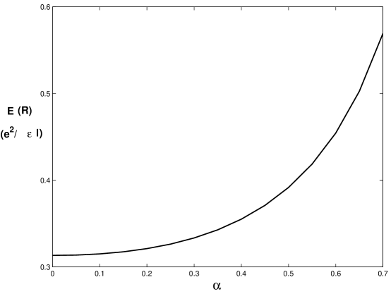
Figure 1: The dependence of skyrmion energy on size with respect to the variation of the parameter $\alpha$ (eqn.(52))

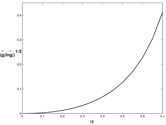
Figure 2: The relationship of $(\tilde{g}|ln\tilde{g}|)^{1/3}$ with $\alpha$ as given by the eqn.(55)

We must mention here that though the value of $\alpha$ is constrained in the region $0\leq\alpha\leq 1$ and $\alpha=1$ corresponds to the hedgehog skyrmion with spin in the radial direction but eqn. (52) suggests that $\alpha=1$ is a singularity point. Indeed, the relation $R=R_{0}(1-\alpha)$ gives a nonzero size for $\alpha=1$ when $R_{0}$ is infinite. So in this case matching the minimum energy for $g=0$, $V=0$ and away from $g=0$ with $g\ll 1$ will not be meaningful. Indeed the solution $\cot{\theta/2}=x/x_{0}$ is valid except for a very narrow region around $x=x_{0}$ by . This implies that a small region around $\alpha=1$ will not give meaningful result for size and energy of the skyrmion. For comparison we have computed the energies of skyrmions in terms of $\alpha$ and it is found that up to $\alpha=0.7$ we have reasonable values of $\tilde{g}$ beyond which $\tilde{g}$ becomes large enough to be compatible with quantum Hall skyrmions [Fig. 1].

This suggests that in spherical geometry within the framework of $O(4)$ nonlinear sigma model in $3+1$ dimensional manifold we can determine the size of the skyrmion incorporating the Skyrme term in the Lagrangian. The ratio of the Zeeman energy and Coulomb energy can be encoded in it [Fig. 2].

It may be added here that very recently Wójs and Quinn qu presented the numerical results for the spin excitation spectra of integral and fractional Hall systems in spherical geometry.

V Discussion

Many authors have considered quantum Hall skyrmions in spherical geometry and studied different aspects of the system in terms of $O(3)$ nonlinear sigma model with success. In all these approaches, the electrons and hence the 3 (constrained) order parameter fields reside on the $2$-dimensional surface of the $2+1$-dimensional $O(3)$ model. To study the static properties of the skyrmions we have used here the $3+1$-dimensional $O(4)$ nonlinear sigma model which actually builds on a different manifold and possesses different number of order parameter fields. The extra order parameter field helps us to consider two independent $SU(2)$ algebras depicting two mutually opposite orientations of the magnetization vector which lives on the $2$-dimensional surface. In this framework with the homotopic analysis we have shown the existence/non-existence of skyrmions in fully polarized, unpolarized and partially polarized quantum Hall states bdp . The Skyrme term which gives rise to the stability of the soliton determines the size of quantum Hall skyrmions. Indeed, the distortion of the spherical shape can be incorporated through the angular dependence which can be conveniently introduced through a parameter $\alpha$ with $0\leq\alpha\leq 1$. Excepting a small region around $\alpha=1$, we can compare the result with the conventional $2D$ formalism when the size is determined by the Zeeman energy and Coulomb energy for small $g$. This helps us to encode the effect of the Zeeman energy and Coulomb energy in the parameter $\alpha$ and the size can be determined from the relation $R=R_{0}(1-\alpha)$ where $R_{0}$ corresponds to the size which is characteristic of the minimum energy $E(R_{0})$. In $2D$ formalism this minimum energy corresponds to $\tilde{g}\ll 1$ which may be matched with the scale invariant value when the energy is contributed by the spin stiffness term for $g=0,V=0$.

We have also shown that the spin and statistics of the skyrmion is given by the $\theta$-term. The skyrmion charge is given by $\nu eZ$ where $Z$ is the winding number associated with the homotopy $\pi_{3}(S^{3})=Z$ and the spin is given by $\nu Z/2$. For $Z=1$, the skyrmion, when moving around a closed loop picks up a phase $2\pi\nu N$ where $N$ is the number of skyrmions enclosed by the loop. In a process which exchanges two skyrmions in the rest frame of one of the skyrmions, the exchange corresponds to the other skyrmion moving about the first in a half circle and hence it picks up a phase $\pi\nu$ which is the statistical phase.

References

- (1) S. C. Zhang, T. H. Hansson and S. Kivelson, Phys. Rev. Lett. 62, 82 (1989).
- (2) D. H. Lee and C. L. Kane, Phys. Rev. Lett. 64, 1313 (1990).
- (3) S. L. Sondhi, A. Karlhede, S. A. Kivelson and E. H. Rezayi, Phys. Rev. B47, 16419 (1993).
- (4) K. Lejnell, A. Karlhede and S. L. Sondhi, Phys. Rev. B59, 10183 (1999).
- (5) T. H. Hansson, A. Karlhede and J. M. Leinaas, Phys. Rev. B54, R11110 (1996).
- (6) S. S. Mandal and V. Ravishankar, Phys. Rev. B57, 12333 (1998).
- (7) X. C. Xie and Song He, Phys. Rev. B53, 1046 (1996).
- (8) B. Basu and P. Bandyopadhyay, Int. J. Mod. Phys. B12, 2649 (1998).
- (9) B. Basu and P. Bandyopadhyay, Int. J. Mod. Phys. B12, 49 (1998).
- (10) S. Dhar, B. Basu and P. Bandyopadhyay, Phys. Lett. A309, 262 (2003).
- (11) B. Basu, S. Dhar and P. Bandyopadhyay : Polarization of Quantum Hall States, Skyrmions and Berry Phase (submitted for publication) : cond-mat/0301368.
- (12) M. Stone, Phys. Rev. B53, 16573 (1996).
- (13) D. Lilliehöök, K. Lejnell, A. Karlhede and S. L. Sondhi, Phys. Rev. B56, 6805 (1997).
- (14) B. Basu, Mod. Phys. Lett. B6, No. 25, 1601 (1992).
- (15) F. D. M. Haldane, Phys. Rev. Lett. 51, 605 (1983).
- (16) Yu. A. Bychkov, A. V. Kolesnikov, T. Maniv and I. D. Vagner, J. Phys. Cond. Matt. 10, 2029 (1998).
-
(17)
T. H. R. Skyrme, Proc. Roy. Soc. A260, 127 (1961);
T. H. R. Skyrme, Nucl. Phys. 31, 556 (1962). - (18) D. Banerjee and P. Bandyopadhyay, J. Math. Phys. 33, 990 (1992).
- (19) A. Wójs and J. J. Quinn, Phys. Rev. B66, 045323 (2002).