Kondo Effect in a Metal with Correlated Conduction Electrons:
Diagrammatic Approach

Abstract

We study the low-temperature behavior of a magnetic impurity which is weakly coupled to correlated conduction electrons. To account for conduction electron interactions a diagrammatic approach in the frame of the 1/N expansion is developed. The method allows us to study various consequences of the conduction electron correlations for the ground state and the low-energy excitations. We analyse the characteristic energy scale in the limit of weak conduction electron interactions. Results are reported for static properties (impurity valence, charge susceptibility, magnetic susceptibility, and specific heat) in the low-temperature limit.

I Introduction

Metals with strongly correlated electrons exhibit highly complex phase diagrams at low temperatures reflecting a rich variety of possible ground states. Prominent examples are the well-known normal Fermi liquid state as well as magnetically ordered, superconducting and insulating phases which may coexist or compete within the same material. A key to a quantitative understanding of the unusual phases is therefore a quantitative description of electronic correlations and their observable consequences.

The present paper focusses on (dilute) magnetic alloys with correlated conduction electrons, i.e., we consider host metals with correlated conduction electrons containing a small amount of magnetic ions. We investigate the question how conduction electron correlations affect the formation of a nonmagnetic Fermi liquid ground state commonly referred to as Kondo effect. The latter has been known to be the source of many anomalous properties in magnetic alloys with noninteracting conduction electrons. In addition to its relevance in magnetic alloys the Kondo effect is becoming important in the study of interacting mesoscopic systems. Theoretical techniques which provide a detailed quantitave understanding of the physical properties of these systems are hence highly desirable. To leading order in the low impurity concentration the electronic properties of dilute magnetic alloys can be calculated in two steps. First one has to determine the elctronic properties of the host which will not be significantly affected by the addition of a small amount of impurities. In the second step the contribution of the magnetic ions has to be calculated.

For a metal with uncorrelated conduction electrons the first part of the problem is solved by standard methods of electronic structure calculation. The theory for the second step is well established [2, 3, 4, 5, 6]. The theoretical techniques available include exact solutions for equilibrium properties as well as approximate methods for dynamic properties. Of particular importance in this context is the diagrammatic approach based upon the large-degeneracy expansion. This scheme can be generalized to the treat non-equilibrium properties which makes it a very flexible method.

The central goal of the present paper to extend the large-degeneracy expansion for the normal-state properties of dilute magnetic alloys to the case of host metals with correlated conduction electrons. In this case, the first step, i. e., the treatment of the host is a highly non-trivial problem which has not yet been solved. Partial answers, however, can be found in limiting cases. Although the diagrammatic approach developped in the present paper is valid for a general conduction electron interaction ( CEI ), we focus on systems where the ground state and the low-energy excitations of the interacting conduction electrons smoothly evolve from those of the non-interacting reference system. This is in marked contrast to the specific behavior encountered in one-dimensional systems. Theoretical studies which have been performed for various models including both impurity spins [7, 8, 9] and Anderson impurities [10, 11, 12] coupled to Luttinger liquids predict rich phase diagrams. Adopting well-established models for the electronic properties of the host, we calculate the evolution of the characteristic energy $T_{K}$ of the low-lying magnetic excitations with the conduction electron repulsion. In the case of uncorrelated conduction electrons the latter is usually much smaller than the typical energy scale of the conduction electrons set by the band width $D$ and depends exponentially on the inverse coupling between the localized electron and the extended conduction states. This fact is a direct consequence of the Fermi liquid ground state realized in normal metals. The diagrammatic approach allows us to explicitly and quantitatively study how the different consequences of electronic correlations (mass renormalization, effective interactions etc) affect the Kondo effect.

The main scope of this paper is to analyze how CEI influence the contribution of magnetic impurities to measurable properties in general and its scaling properties in particular. We calculate thermodynamic properties (impurity valence, charge susceptibiliy, magnetic susceptibility and specific heat) in the low-teperature limit to leading order in the inverse degeneracy.

Recent calculations for a magnetic impurity in a metal with interacting conduction electrons [13, 14] adopted either the DMFT approach [15] or the NRG but for a very special model [16]. The model calculations mentioned above predict non-trivial variation with the Coulomb repulsion of the characteristic temperature $T_{K}$.

Generally, the modifications introduced by the conduction electron interactions (CEI ) into the low-energy excitations arise from the subtle interplay of three different types of influences. First, the density of conduction states at the Fermi level is changed. Second, the probability for virtual transitions between impurity and conduction states are reduced by the on-site Coulomb interaction $U$. Third, the effective spin coupling between the conduction and impurity electrons is enhanced by the increased number of uncompensated spins in the correlated conduction electron system. Considering these facts, it is not surprising that model studies accounting only for selected aspects arrive at rather controversial conclusions concerning the Kondo effect in metals with correlated electrons [17, 18, 19]. The Kondo spin model generalised to the case of the interacting conduction-electron host was discussed in [17] and it was shown there that two-particle Green’s functions of host electrons ( vertex corrections ) are an essential component of the theory which leads to an enhancement of the exponential Kondo scale for a weak CEI. This enhancement may be traced to the third type of effects caused by the CEI. The ground state energy of the Anderson impurity for weak CEI was considered in the frame of $1/N$ expansion [18]. The same enhancement of the exponential Kondo scale, formally due to the renormalization increase of the hybridization width $\Delta$, appears in this work [18]. In contrast to the above-mentioned findings a decrease of $T_{K}$ due to the CEI in the Hubbard model was reported in the paper [19]. This decrease is a consequence of the change in the single electron properties of conduction electrons caused by the interaction $U$ ( including the change of the chemical potential as the function of $U$  ). The vertex corrections influence which renormalizes both parameters of the Anderson impurity model[20], $\epsilon_{f}$ and $\Delta$ are not considered in [19]. At this point, we should like to mention that the role of the Coulomb interaction between the magnetic impurity electron and conduction electrons, $U_{fc}$, was broadly discussed. We do not discuss here the Coulomb interaction between localized and conduction electrons which is considered in its various aspects in [21, 22, 23, 24, 25]. It was shown that its effect at $U_{fc}\ll U_{f}$ may be fully absorbed by the renormalization of two parameters of the Anderson impurity Hamiltonian: the impurity electron energy level $\epsilon_{f}$ and the hybridization width $\Delta$. In the following we assume that the on-site impurity electron Coulomb repulsion $U_{f}$ is very large, $U_{f}\rightarrow\infty$, and we do not take into account explicitly the $U_{fc}$ interaction.

The paper is organized as follows: In Section II we begin with a discussion of the Hamiltonian for an Anderson impurity embedded in a metallic host with correlated conduction electrons and the extension of the standard selfconsistent large-degeneracy approximation to the case of CEI. Both the interaction-induced changes in the single-electron spectral function of interacting conduction electrons and their vertex function are included. In Section III expressions for configurational selfenergies together with the NCA integral equations are formulated for a general case of CEI. The expressions are evaluated in Section IV for a model where the Coulomb vertex function is only weakly frequency-dependent. Thermodinamic properties at zero temperature are presented in Section V and Section VI contains discussions and summary. Technical details related to the explicit evaluation of diagrams and discussions of the fourth-order hybridisation coupling are in the appendices. Some of the results appeared in the short unpublished preprint [20].

II Model and calculational scheme

We adopt a generalized Anderson model for a magnetic impurity coupled to interacting conduction electrons. The resulting Hamiltonian reads

$$H=H_{band}+H_{imp}+H_{mix}$$ (1)

where the three components describe the conduction electrons, the f states and a hybridization or mixing interaction between the two

$$H_{band} = \sum_{\vec{k}\sigma}\epsilon_{\vec{k}}c_{\vec{k}\sigma}^{\dagger}c_{\vec{k}\sigma}+H_{CEI}$$ (2)

$$H_{imp} = \sum_{m}\epsilon_{f}n_{fm}+{U_{f}\over 2}\sum_{m\neq m{\prime}}n_{fm}n_{fm^{\prime}}$$ (3)

$$H_{mix} = \sum_{\vec{k},m,\sigma}\left(V_{m\sigma}(\vec{k})f_{m}^{\dagger}c_{\vec{k}\sigma}+h.c.\right)\quad.$$ (4)

The creation (annihilation) operators for conduction electrons with momentum $\vec{k}$, band energy $\epsilon_{\vec{k}}$ and spin $\sigma$ are denoted by $c_{\vec{k}\sigma}^{\dagger}(c_{\vec{k}\sigma})$. Throughout this paper, all energies are measured relative to the Fermi level. The conduction states are assumed to be orbitally non-degenerate. Their interaction is accounted for by

$$H_{CEI} = {1\over 2L}\sum_{\vec{k},\vec{k}^{\prime},\vec{q}\ \sigma,\sigma^{\prime}}U(\vec{k}+\vec{q},\vec{k}^{\prime}-\vec{q};\vec{k}^{\prime},\vec{k})$$ (6)

$$\;\;\;\;\;\;\;\;\;\;\;\;\;\;\;\;\;\;\;\times c_{{\vec{k}+\vec{q}}\sigma}^{\dagger}c_{\vec{k}^{\prime}-\vec{q}\sigma^{\prime}}^{\dagger}c_{\vec{k}^{\prime}\sigma^{\prime}}c_{\vec{k}\sigma}.$$

where $L$ is the number of lattice sites. In the present paper, we approximate $H_{CEI}$ by a Hubbard-type interaction

$$U(\vec{k}+\vec{q},\vec{k}^{\prime}-\vec{q};\vec{k}^{\prime},\vec{k})\rightarrow U$$ (7)

where $U$ denotes the local Coulomb repulsion between two conductionelectrons at the same lattice site. Another important example which shall be studied in a forthcoming paper are Fermi liquid systems where the CEI renormalizes the quasiparticle dispersion $\epsilon_{\vec{k}}$ and also introduces a ‘residual’ interaction among them.

The $f_{m}^{\dagger}(f_{m})$ are the creation (annihilation) operators for $f$-electrons at the impurity site. They are characterized by the total angular momentum $J$ and a quantum number $m$ which denotes the different states $m=1,\dots,N$ within the $N$-fold degenerate ground state multiplet with orbital energy $\epsilon_{f}$. The Coulomb repulsion $U_{f}$ between two $f$-electrons at the impurity site is assumed to be much larger than the other energy scales and therefore we may let $U_{f}\rightarrow\infty$. For simplicity we do not include here excited multiplet states, ignore crystal electric field splittings and assume that the impurity has only one electron ( hole  ) in its magnetic configuration. We account for the large Coulomb interaction among the f-electrons $U_{f}\rightarrow\infty$ by restricting the Hilbert space, i. e., by removing all states in which the f occupancy exceeds unity.

The mixing between the two subsystems is conveniently characterized by the ”hybridization width”[26]

$$\Delta(E)=\pi\frac{1}{L}\frac{1}{N}\sum_{\vec{k}\ \sigma\ m}\left|V_{m\sigma}(\vec{k})\right|^{2}\ \delta(E-\epsilon_{\vec{k}})\quad.$$ (8)

We are mainly interested in the regime $\left|\epsilon_{f}\right|\gg\Delta_{m}(0)$ which is usually referred as ”local moment regime”.

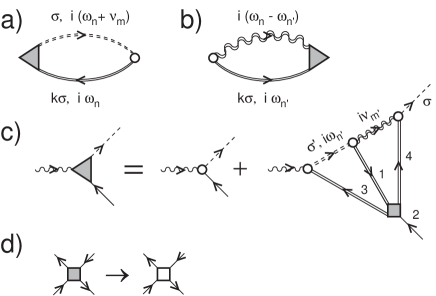
FIG. 1.: Self-consistent f configuration self-energies and contributions to the vertex. The solid, dashed and wavy lines represent the dressed propagators for conduction electrons, occupied and empty f states. The open circle denotes the bare hybridization V while open and filled squares are the bare on-site Coulomb repulsion and the two-particle vertex $\Gamma_{\sigma,\bar{\sigma}}^{(U)}(1,2;3,4)$, respectively. (a) Empty state self-energy $\Sigma_{0}(i\nu_{m})$. (b) Occupied state self-energy $\Sigma_{\sigma}(i\omega_{n})$. (c) Contribution to the effective hybridization vertex. (d) Lowest order correction.

The central goal is to calculate the impurity contribution to the low-energy properties of the dilute magnetic alloy. The latter are given in terms of the Green’s functions for the empty f-state $|0>$ ($4f^{0}$- configuration) and the occupied $f$ states $|m>$ ($4f^{1}$- configuration) denoted by $G_{0}(z)$ and $G_{m}(z)$, respectively,

$$G_{0}(z)\;=\;{1\over{z-\Sigma_{0}(z)}}\qquad;\qquad G_{m}(z)\;=\;{1\over{z-\epsilon_{f}-\Sigma_{m}(z)}}\quad.$$ (9)

They are coupled through the configurational selfenergies $\Sigma_{0}(z)$ and and $\Sigma_{m}(z)$ for which we derive expressions proceeding in close analogy to the case of non-interacting conduction electrons.

The electronic properties of the metallic host are not affected by the presence of a small amount of magnetic impurities. To leading order in the small concentration they are characterized by the $1$- and $2$-particle Green’s function describing the single-particle excitations and the two-particle correlations of the interacting conduction electrons, respectively.

We assume that the single-electron Green’s function

$$G_{\sigma}(\vec{k},z)=\frac{1}{z-\epsilon_{\vec{k}}-\Sigma_{\sigma}(\vec{k},z)}$$ (10)

as well as the conduction electron selfenergy $\Sigma_{\sigma}(\vec{k},z)$ do not explicitly depend upon the wave vector $\vec{k}$ but vary with $\vec{k}$ mainly through the bare band energy, i.e.

$$G_{\sigma}(\vec{k},z)=G_{\sigma}(\epsilon_{\vec{k}},z)\qquad;\qquad\Sigma_{\sigma}(\vec{k},z)=\Sigma_{\sigma}(\epsilon_{\vec{k}},z)\quad.$$ (11)

This condition is always satisfied in the DMFT approach [15] where the dominant many-body effects are included in a local selfenergy. As a consequence, also the general n-particle Green’s functions of the conduction electron system depend upon the wave vectors through the corresponding band energies.

The configurational self-energies $\Sigma_{0}$ and $\Sigma_{m}$ are derived by means of a perturbation expansion in terms of Green’s functions for the f-configurations, 1- and 2-particle Green’s functions for the interacting conduction electrons as well as (bare) hybridization vertices. The rules for constructing and evaluating the empty- and occupied-state selfenergies in the restricted Hilbert space of the infinite-U-Anderson model are summarized in [27]. Typical contributions to the f-configurational selfenergies are displayed in Figure 1. These include the non-crossing diagrams Figure 1(a) und (b) where the conduction electron interactions enter through the fully renormalized conduction electron propagator. The diagrams 1(c) and (d) describe vertex corrections. We shall show below that under the assumptions Eq. (11) the infinite-order summation of these diagrams based on the self-consistent approximation for the empty- and occupied-f-state propagators can be considered as the leading order contribution in the inverse degeneracy $1/N$. The remaining part of the present section is devoted to the justification of this conjecture.

We start by briefly summarizing the basic facts on which the large-degeneracy expansion is based in the case of non-interacting conduction electrons. The classification scheme exploits the fact that the bare conduction electron propagator $1/(z-\epsilon_{\vec{k}})$ depends upon the wave vector $\vec{k}$ through the bare band energy. As a consequence, the summations over internal $\vec{k}$-vectors can be decomposed into integrals over the (bare) band energies $\epsilon$ and averages over constant energy surfaces according to

$${1\over L}\sum_{\vec{k}}\dots\rightarrow\int d\epsilon\,\,{1\over L}\sum_{\vec{k}}\delta(\epsilon-\epsilon_{\vec{k}})\dots=\int d\epsilon\,\,N(\epsilon)\langle\dots\rangle_{\epsilon}$$ (12)

Here $N(\epsilon)$ is the density of bare band energies. The $\vec{k}$-averages $\langle\dots\rangle_{\epsilon}$ which contain only combinations of the hybridization matrix elements

$$<V^{*}_{m\sigma}(\vec{k})V_{m^{\prime}\sigma}(\vec{k})>_{\epsilon}=$$ (13)

$${1\over{N(\epsilon)}}\left\{{1\over L}\sum_{\vec{k}\sigma}V^{*}_{m\sigma}(\vec{k})V_{m^{\prime}\sigma}(\vec{k})\delta(\epsilon-\epsilon_{\vec{k}})\right\}\sim V^{2}_{m}(\epsilon)\delta_{mm^{\prime}}$$ (14)

provide the $m$-selection rule [28] which simplifies the structure of the selfenergy contributions and ultimately allows for a classification with respect to the small parameter $1/N$.

¿From the preceding discussion it is apparent that the assumption Eq. (11) guarantees the validity of the $1/N$ classification scheme for all diagrams where the conduction electron properties enter via the single-particle Green’s function. Within this subclass the contributions displayed in Figure 1(a) and (b) ( without vertex corrections ) are the leading ones with respect to the small parameter $1/N$.

To assess the validity of the $1/N$ expansion is more subtle for the diagrams containing the two-particle Green’s function. Here the simplifying assumptions Eq. (11) imply ( see Section III ) that the hybridization matrix elements enter diagrams in Figure 1( a,c ) and ( b,c ) in the combination

$$V^{(4)}(E_{1}\sigma_{1},E_{2}\sigma_{2};E_{3}\sigma_{3},E_{4}\sigma_{4})=\frac{1}{L^{3}}\sum_{\vec{k}_{1},\vec{k}_{2},\vec{k}_{3},\vec{k}_{4}}$$ (15)

$$\delta(E_{1}-\epsilon(\vec{k}_{1}))\delta(E_{2}-\epsilon({\vec{k}_{2}}))\delta(E_{3}-\epsilon({\vec{k}_{3}}))\delta(E_{4}-\epsilon({\vec{k}_{4}}))$$ (16)

$$\sum_{m,m^{\prime}}\ V_{m\sigma_{1}}(\vec{k}_{1})V_{m^{\prime}\sigma_{2}}(\vec{k}_{2})V_{m\sigma_{3}}^{\ast}(\vec{k}_{3})V_{m^{\prime}\sigma_{4}}^{\ast}(\vec{k}_{4})$$ (17)

$$\delta^{*}(\vec{k}_{3}+\vec{k}_{4}-\vec{k}_{1}-\vec{k}_{2})\quad.$$ (18)

where the Laue function

$$\delta^{*}(\vec{k}_{1}\!+\!\vec{k}_{2}\!-\!\vec{k}_{3}\!-\!\vec{k}_{4})=\frac{1}{L}\sum_{\vec{R}_{n}}\exp\left\{i\left(\vec{k}_{1}\!+\!\vec{k}_{2}\!-\!\vec{k}_{3}\!-\!\vec{k}_{4}\right)\right\}$$ (19)

accounts for momentum conservation up to a reciprocal lattice vector.

In the Appendix A we present a detailed model calculation for a rare earth impurity hybridized with tight-binding $s$-band states. The results show that the new contributions to $\Sigma_{0}$ and $\Sigma_{m}$ are $O(1)$ and $O(1/N)$, i. e. , of the same order of magnitude with respect to $1/N$ as their NCA counterparts. It is interesting to note that the dominant contributions to $V^{(4)}$ are non-local coming from the coupling of the $f$-states to the conduction electrons at the neighboring sites.

To summarize, the configurational selfenergies displayed in Figure 1 provide a consistent extension of the well-known selfconsistent large-degeneracy expansion to the case of interacting conduction electrons. Actual calculations, however, require the fully renormalized conduction-electron propagator as well as the Coulomb vertex. Since this problem still remains unsolved for the Hubbard model [29, 30] we have to adopt approximate expressions derived either from phenomenological considerations or from partial resummation of selected classes of diagrams.

General qualitative results can be derived in limiting cases. Prominent among them is the case where the Coulomb vertex can be considered as a static quantity which includes the limit of weakly interacting conduction electrons as well as the Fermi liquid case.

III Configurational selfenergies

For non-interacting conduction electrons, the self-consistent solution [31, 27] has three characteristic features: The occupied f-spectrum shifts to peak at a value ${\bar{\epsilon}}_{f}\simeq\epsilon_{f}+\Re\Sigma_{m}(\epsilon_{f})$, the dominant contribution to the level shift coming from the continuum of charge fluctuations. The resonance in the occupied f-spectral function acquires a small width. Finally, the empty state spectral function exhibits a pronounced structure at $\omega_{0}={\bar{\epsilon}}_{f}-T_{K}$ which develops with decreasing temperature and which sets the scale for the low-temperature behavior. This feature is the direct manifestation of the Kondo effect reflecting the admixture of $f^{0}$-contributions to the ground state and the low-energy excitations.

In this paper, we study the influence of the CEI on this non-perturbative feature. Of particular interest are the position of the resonance energy $\omega_{0}$ relative to the energy ${\bar{\epsilon}}_{f}$ of the $4f^{1}$ configuration as well as the weight of the resonance.

Let us first neglect vertex corrections and focus on the modifications introduced by the CEI into the single-particle excitations of the conduction electron system. They are accounted for by inserting the full conduction electron propagator for interacting electrons $G_{\sigma}(\vec{k},i\omega_{n})$ from Eq. (10) into the configurational selfenergies Figure 1(a,b).

The selfenergy of the occupied f-level

$$\Sigma_{m}^{(0)}\left(\omega\right) = \frac{1}{L}\sum_{\vec{k}\sigma}V_{m\sigma}(\vec{k})\!\!\int dE\,\,n_{f}(-E)A_{\sigma}(\vec{k},E)$$ (21)

$$\;\;\;\;\;\;\;\;\;\;\;\;\;\;\;\;\;\;\;\;\;\;\;\;\times G_{0}\left(\omega-E\right)V_{m\sigma}^{*}(\vec{k})$$

$$= \frac{1}{\pi}\!\!\int dE\,\,\Delta_{m}^{0}(E)n_{f}(-E)G_{0}(\omega-E)$$ (22)

is diagonal in $m$ as shown in the previous section. Here $n_{f}(E)$ denotes the Fermi function. The properties of the metallic host are reflected in the energy-dependent hybridization strength

$$\Delta_{m}^{(0)}(E)=\frac{1}{L}\sum_{\vec{k}\sigma}V_{m\sigma}(\vec{k})A_{\sigma}(\vec{k},E)V_{m\sigma}^{*}(\vec{k})$$ (23)

where the conduction electron spectral function $A_{\sigma}(\vec{k},E)=-\frac{1}{\pi}ImG_{\sigma}(\vec{k},E)$ depends upon the wave vector $\vec{k}$ mainly through the band energy $\epsilon_{\vec{k}}$ ( see Eq. (11) ). The selfenergy of the empty state is treated in the same manner so the corresponding selfenergy expressions reduce to

$$\Sigma_{0}^{(0)}\left(\omega\right) = {1\over\pi}\sum_{m}\int dE\,\,\Delta_{m}^{(0)}(E)n_{f}(E)G_{m}\left(\omega+E\right)$$ (24)

$$\Sigma_{m}^{(0)}\left(\omega\right) = {1\over\pi}\int dE\,\,\Delta_{m}^{(0)}(E)n_{f}(-E)G_{0}\left(\omega-E\right)$$ (25)

in close analogy to the case of non-interacting electrons [31].

The selfconsistency equations Eq. (25) were solved numerically [32] for various well-established approximations to the spectral function of interacting conduction electrons such as the Hubbard III model [33] and the Roth approximation [34]. The general results can be summarized as follows: It is obvious that for (weakly) interacting conduction electrons the dominant effect of hybridization on the $4f^{1}$ configurational spectrum is a shift $\epsilon_{f}(U)-\epsilon_{f}\simeq\Re\Sigma_{m}(\epsilon_{f})$ of the resonance energy which is renormalized by the Coulomb repulsion $U$ and its influence on the charge fluctuations. The quantity of interest, however, is the empty-state selfenergy and its variation with energy in the vicinity of $\epsilon_{f}$ which can be deduced from rather simple considerations assuming that the CEI do not introduce anomalies into the conduction electron spectral function on the energy scale defined by the characteristic temperature $T_{K}$. The smooth variation with energy of $\sum_{\vec{k}}A_{\sigma}(\vec{k},E)$ implies that in the metallic state the basic analytic structure of $\Sigma_{0}^{(0)}(\omega)$ is not altered as compared to the case of non-interacting conduction electrons, the characteristic feature being a logarithmic variation in the vicinity of the f-energy $\epsilon_{f}$. The prefactor, however, is proportional to the interaction-renormalized density of states at the Fermi level $N(\epsilon_{f})$. The low-energy scale, $T_{K}$, i.e. the distance between the pole in the empty f-state Green’s function and the $4f^{1}$ peak depends on the renormalized parameters in the usual exponential way. Especially the above is clear for the case when the CEI leads to the spectral function of the quasipartical type, $A_{\sigma}(\vec{k},E)$ = $\delta(E-{\bar{\epsilon}}_{\vec{k}})$ with a new dispersion ${\bar{\epsilon}}_{\vec{k}}$.

Would the single-electron contribution presents the whole story the CEI-case would be relatively simple. The Coulomb interaction induces vertex corrections which are of the same order in the inverse degeneracy $1/N$ as the preceding single electron contributions. They are an important ingredient of the theory and must be included in the discussion [17, 20].

The explicit calculation requires the full Coulomb vertex $\Gamma^{(U)}$ of the conduction electrons as input which must be determined consistently with the conduction-electron self-energy. We evaluate the vertex corrections by analytic continuation from the Matsubara frequencies inserting the spectral representation

$$G_{\sigma}(\vec{k},i\omega_{m})=\int dE\,\frac{A_{\sigma}(\vec{k},E)}{i\omega_{m}-E}$$ (26)

for the conduction electron propagators and following the rules specified in [27]. The projection onto the relevant physical subspace is performed implicitly in the summation over the Matsubara frequencies where we retain only the contributions from the poles in the conduction electron propagators. The empty state self-energy, $\Sigma_{0}^{(U)}\left(\omega\right)$, (see Figure (1, a, c))can be written as

$$\Sigma_{0}^{(U)}\left(\omega\right) = \frac{1}{\pi}\sum_{m}\,\int dE\,\,\Delta_{0,m}^{(U)}(E,\omega)n_{f}(E)G_{m}(\omega+E)$$ (27)

where the Coulomb contribution to the hybridization strength is given by

$$\Delta_{0,m}^{(U)}\left(E,\omega\right) = \pi{1\over L}\sum_{\vec{k}\sigma}A_{\sigma}(\vec{k},E)\frac{1}{L^{2}}\sum_{\vec{k}_{1}\sigma_{1}}\!\!\,\,\int d\Omega\,\,n_{f}(-E+\Omega)A_{\sigma_{1}}(\vec{k}_{1},E-\Omega)G_{0}\left(\omega+\Omega\right)$$ (32)

$$\sum_{\vec{k}_{2}\sigma_{2}}\!\!\sum_{\vec{k}^{\prime}\sigma^{\prime}}\!\!\,\,\sum_{m^{\prime}}\int dE^{\prime}\,\,G_{m^{\prime}}\left(\omega+E^{\prime}+\Omega\right)$$

$$\left\{A_{\sigma_{2}}(\vec{k}_{2},E^{\prime}+\Omega)n_{f}(E^{\prime}+\Omega)G_{\sigma^{\prime}}\left(\vec{k}^{\prime},E^{\prime}\right)+A_{\sigma^{\prime}}(\vec{k}^{\prime},E^{\prime})n_{f}(E^{\prime})G_{\sigma_{2}}\left(\vec{k}_{2},E^{\prime}+\Omega\right)\right\}$$

$$\left(V_{m\sigma_{1}}(\vec{k}_{1})V_{m^{\prime}\sigma_{2}}(\vec{k}_{2})V_{m\sigma}^{*}(\vec{k})V_{m^{\prime}\sigma^{\prime}}(\vec{k}^{\prime})^{*}\Gamma_{\sigma_{1}\sigma_{2};\sigma\sigma^{\prime}}^{(U)}\left(\vec{k}_{1}E-\Omega,\vec{k}_{2}E^{\prime}+\Omega;\vec{k}E,\vec{k}^{\prime}E^{\prime}\right)+c.c\right)$$

$$\delta^{*}\left(\vec{k}_{1}+\vec{k}_{2}-\vec{k}-\vec{k}^{\prime}\right)$$

Here and elsewhere $\Gamma_{\sigma_{1}\sigma_{2};\sigma_{3}\sigma_{4}}^{(U)}\left(1,2;3,4\right)$ is the Coulomb vertex corrections with indices 1,2 for in- and 3,4 for outgoing particles. A similar expression is found for the hybridization strength entering the occupied-f-states selfenergies, ( see Figure (1, b, c )

$$\Sigma_{m}^{(U)}\left(\omega\right) = \frac{1}{\pi}\int dE\,\,\Delta_{m,m}^{(U)}(E,\omega)n_{f}(-E)G_{0}(\omega-E)$$ (33)

with

$$\Delta_{m,m}^{(U)}\left(E,\omega\right) = \pi{1\over L}\sum_{\vec{k}\sigma}A_{\sigma}(\vec{k},E)\frac{1}{L^{2}}\sum_{\vec{k}_{1}\sigma_{1}}\!\!\,\,\sum_{m^{\prime}}\int d\Omega\,\,n_{f}(E-\Omega)A_{\sigma_{1}}(\vec{k}_{1},E-\Omega)G_{m^{\prime}}\left(\omega-\Omega\right)$$ (38)

$$\sum_{\vec{k}_{2}\sigma_{2}}\!\!\sum_{\vec{k}^{\prime}\sigma^{\prime}}\!\!\,\,\int dE^{\prime}\,\,G_{0}\left(\omega-E^{\prime}-\Omega\right)$$

$$\left\{A_{\sigma_{2}}(\vec{k}_{2},E^{\prime}+\Omega)n_{f}(-E^{\prime}-\Omega)G_{\sigma^{\prime}}\left(\vec{k}^{\prime},E^{\prime}\right)+A_{\sigma^{\prime}}(\vec{k}^{\prime},E^{\prime})n_{f}(-E^{\prime})G_{\sigma_{2}}\left(\vec{k}_{2},E^{\prime}+\Omega\right)\right\}$$

$$\left(V_{m\sigma}(\vec{k})V_{m^{\prime}\sigma^{\prime}}(\vec{k}^{\prime})V_{m\sigma_{1}}^{*}(\vec{k}_{1})V_{m^{\prime}\sigma_{2}}^{*}(\vec{k}_{2})\Gamma_{\sigma\sigma^{\prime};\sigma_{1}\sigma_{2}}^{(U)}\left(\vec{k}E,\vec{k}^{\prime}E^{\prime};\vec{k}_{1}E-\Omega,\vec{k}_{2}E^{\prime}+\Omega\right)+c.c\right)$$

$$\delta^{*}\left(\vec{k}_{1}+\vec{k}_{2}-\vec{k}-\vec{k}^{\prime}\right)$$

Note that the self-consistency equations, Eq. (25) generalized by including the vertex correction contributions from Eqs. (32, 38) in the integrands of Eq. (25) read

$$\Sigma_{0}\left(\omega\right)={1\over\pi}\sum_{m}\int dE\,\,(\Delta_{m}^{(0)}(E) +$$ (39)

$$\Delta_{0,m}^{(U)}(E,\omega))n_{f}(E)G_{m}\left(\omega+E\right)$$ (40)

$$\Sigma_{m}\left(\omega\right)={1\over\pi}\int dE\,\,(\Delta_{m}^{(0)}(E) +$$ (41)

$$\Delta_{m,m}^{(U)}(E,\omega))n_{f}(-E)G_{0}\left(\omega-E\right)$$ (42)

Eqs. (32, 38) are general in the sense that they do not assume any specific form of conduction electrons spectral functions, vertex corrections, etc.. In the case when $\vec{k}$- dependences in conduction electron propagators enter as in Eq. (11) only via the conduction eletrons dispersion $\epsilon(\vec{k})$ Eq. (32) may be casted in the form

$$\Delta_{0,m}^{(U)}(E,\omega))=\int d\omega_{1}d\omega_{2}d\omega_{3}d\omega_{4}\,\,\sum_{\sigma_{1}\sigma_{2}\sigma_{3}\sigma_{4}}$$ (43)

$$V_{m}^{(4)}(\sigma_{1}\omega_{1},\sigma_{2}\omega_{2},\sigma_{3}\omega_{3},\sigma_{4}\omega_{4})$$ (44)

$$F_{m}(E,\omega,\sigma_{1}\omega_{1},\sigma_{2}\omega_{2},\sigma_{3}\omega_{3},\sigma_{4}\omega_{4})$$ (45)

Here $V_{m}^{(4)}$ denotes the 4-order hybridization coupling given explicitly in Eq. (18) while $F_{m}(E,\omega,\sigma_{1}\omega_{1},\sigma_{2}\omega_{2},\sigma_{3}\omega_{3},\sigma_{4}\omega_{4})$ is readily obtained by using Eq. (11). Eq. (22) is simplified enormously in the case when conduction electrons spectral functions may be approximated by the quasiparticle spectra . A similar coupling $V_{m}^{(4)}$ may be introduced for the $\Delta_{mm}^{(U)}(E,\omega)$. For a model calculation of the 4-order hybridization coupling $V_{m}^{(4)}$ see Appendix A.

To summarize, we generalized the selfconsistent large degeneracy expansion to the case of correlated conduction electrons. The modifications due to the interaction enter via the spectral function of the conduction electrons as well as an effective renormalized hybridization vertex. The explicit evaluation hence requires these quantities for a system of interacting conduction electrons. In the subsequent sections, we shall consider the influence of the Coulomb repulsion $U$ on the effective hybridization strengths which depend upon both $E$ and $\omega$. In particular, we shall discuss the analytic structure of the selfenergies for weakly interacting electrons and discuss the modifications in observable properties in the low-temperature limit $T\rightarrow 0$.

IV Weak Conduction-Electron Interaction

As a first example, we consider the limit of weakly interacting electrons, i. e. , we assume the Coulomb repulsion $U$ to be much smaller than the bandwidth $D$. To leading order in the small ratio $U/D\ll 1$ we can neglect changes in the spectral function of the conduction electrons which we assume to be given by

$$A_{\sigma}(\vec{k},E)\longrightarrow\delta(E-\epsilon(\vec{k}))\quad.$$ (46)

The central focus of the present paper is the lowest pole $\omega_{0}$ of the empty-f state Green’s function

$$\omega_{0}-\Sigma_{0}^{(0)}(\omega_{0})-\Sigma_{0}^{(U)}(\omega_{0})\;=\;0$$ (47)

and its variation with the Coulomb repulsion $U$.

The Coulomb repulsion contributes to the configurational selfenergies via the effective hybridization strengths Eq. (32) and Eq. (38) where the full Coulomb vertex is replaced by the bare local non-retarded repulsion ( see Figure 1, d )

$$\Gamma_{\sigma_{1}\sigma_{2};\sigma\sigma^{\prime}}^{(U)}\left(\vec{k}_{1}E-\Omega,\vec{k}_{2}E^{\prime}+\Omega;\vec{k}E,\vec{k}^{\prime}E^{\prime}\right)\longrightarrow$$ (48)

$$U\frac{1}{2}\left(i\sigma_{y}\right)_{\sigma_{1}\sigma_{2}}\left(i\sigma_{y}\right)_{\sigma\sigma^{\prime}}$$ (49)

for the case of $\Delta_{0,m}^{(U)}$ and

$$\Gamma_{\sigma\sigma^{\prime};\sigma_{1}\sigma_{2}}^{(U)}\left(\vec{k}E,\vec{k}^{\prime}E^{\prime};\vec{k}_{1}E-\Omega,\vec{k}_{2}E^{\prime}+\Omega\right)\longrightarrow$$ (50)

$$U\frac{1}{2}\left(i\sigma_{y}\right)_{\sigma\sigma_{1}}\left(i\sigma_{y}\right)_{\sigma^{\prime}\sigma_{2}}\quad.$$ (51)

for the case of $\Delta_{m,m}^{(U)}$ accordingly.

We elaborate on the selfenergies expressions, Eqs. (27, 33), for the case of an orbitally non-degenerate Anderson model. In this case the hybridisation matrix element reduces to $V_{m\sigma}(\vec{k})=\delta_{m\sigma}V(\vec{k})$ and the occupied f-state propagator does not depend upon the m-index[35].

Inserting Eqs. (46, 48, 50) into the vertex corrections Eq. (32) and Eq. (38) correspondingly we obtain

$$\Delta_{0,m}^{(U)}\left(E,\omega\right) = \pi U\int dE_{1}\,dE_{2}\,dE^{\prime}n_{f}(-E_{1})G_{0}\left(\omega+E-E_{1}\right)\frac{2\Re{V^{(4)}(E_{1},E_{2},E,E^{\prime})}}{E_{1}+E_{2}-E-E^{\prime}}$$ (53)

$$\left\{G_{m}\left(\omega+E_{2}\right)n_{f}(E_{2})-G_{m}\left(\omega+E^{\prime}+E-E_{1}\right)n_{f}(E^{\prime})\right\}$$

and

$$\Delta_{m,m}^{(U)}\left(E,\omega\right) = \pi U\int dE^{\prime}\,dE_{3}\,dE_{4}n_{f}(E_{3})G_{-m}\left(\omega+E_{3}-E\right)\frac{2\Re{V^{(4)}(E,E^{\prime},E_{3},E_{4})}}{E_{3}+E_{4}-E-E^{\prime}}$$ (55)

$$\left\{G_{0}\left(\omega-E_{4}\right)n_{f}(-E_{4})-G_{0}\left(\omega+E_{3}-E-E^{\prime}\right)n_{f}(-E^{\prime})\right\}\qquad.$$

To derive these expressions we used Eq. (18), performed the $\sigma$-summations and the relevant integrations.

The hybridization matrix elements $V_{\vec{k}}$ vary smoothly with $\left|\vec{k}\right|$, and, as a consequence, $V_{m}^{(4)}(E_{1},E_{2},E_{3},E_{4})$ is a smooth function of the energies $E_{i}\quad i=1,\dots,4$. It can be approximated by (see Appendix A)

$$V_{m}^{(4)}(E_{1},E_{2},E_{3},E_{4})\longrightarrow\left(\frac{N(0)\Delta}{\pi}\right)^{2}\longrightarrow\left(\frac{\Delta}{2\pi D}\right)^{2}$$ (56)

where $\Delta$ is the hybridization width. In the following we shall adopt a flat density of states extending over the energy range $(-D,D)$ and use for the $V_{m}^{(4)}$ the last expression in Eq. (56).

We start by discussing the configurational selfenergies for $T=0$ where the Fermi function can be replaced by the step function $n_{f}(x)=\theta(-x)$ and we insert the free propagator for the occupied-state Green’s function [36]

$$G_{m}(\omega)\rightarrow\frac{1}{\omega-\epsilon_{f}}\quad.$$ (57)

The selfenergies $\Sigma_{0}^{(U)}$ and $\Sigma_{m}^{(U)}$ can be expressed in terms of three integrals $I_{0i}$ and $I_{mi}$, $1=1,2,3$, respectively,

$$\Sigma_{0}^{(U)}\left(\omega\right)=\frac{1}{2\pi^{2}}U\left(\frac{\Delta}{D}\right)^{2}$$ (58)

$$\left(-I_{01}(\omega)\ln\left[\frac{\omega-\epsilon_{f}}{\omega-\epsilon_{f}-D}\right]+I_{02}(\omega)+I_{03}(\omega)\right)$$ (59)

and

$$\Sigma_{m}^{(U)}\left(\omega\right)=-\frac{1}{4\pi^{2}}U\left(\frac{\Delta}{D}\right)^{2}$$ (60)

$$\left(-I_{m1}(\omega)\ln\left[\frac{\omega}{\omega-D}\right]+I_{m2}(\omega)+I_{m3}(\omega)\right).$$ (61)

Further we discuss the half-filling case[38]. This particular choice of the band filling, however, does not affect the analytic behavior in the energy range of interest, i. e. , for $\omega\simeq\epsilon_{f}$.

We should like to emphasize that the integrals $I_{0i}$ and $I_{mi}$ in Eqs. (59) and (61) depend upon the full empty-state Green’s function $G_{0}(\omega)$. This fact implies that the Coulomb contribution to the selfenergy, $\Sigma_{0}^{(U)}(\omega)$, has to be determined selfconsistently from Eq. (59) in principle. In the present paper, we employ an iterative scheme and adopt a convenient parametrization of the spectral functions $A_{0}(\omega)$ and . Before presenting the results, let us briefly summarize our procedure. In the first step, we insert the free empty-state propagator, i.e., $A_{0}(\omega)\rightarrow\delta(\omega)$ into the rhs of Eq. (59). The resulting selfenergy $\Sigma_{0}^{(U)}(\omega)$ yields a Green’s function $G_{0}(\omega)$ which has a Kondo-type pole at $\omega_{0c}(U)<\omega_{0}(U=0)<\epsilon_{f}$ with rather small weight $1-n_{fc}(U)$. The index c denotes the fact that only the charge fluctuation contribution was included in the selfenergy $\Sigma_{0c}^{(U)}(\omega)$. In the next iteration, we account for the low-energy peak in the spectral function which we model by two $\delta$-functions $A_{0}(\omega)\rightarrow(1-n_{fc}(U))\delta(\omega-\omega_{0c}(U))+n_{fc}(U)\delta(\omega)$. Including the low-energy spin fluctuations furthers shifts the threshold $\omega_{0}(U)$ to lower energy, i.e. we find $\omega_{0}(U)<\omega_{0c}(U)<\omega_{0}(U=0)<\epsilon_{f}$.

Modelling the spectral function $A_{0}(\omega)$ by a combination of $\delta$-functions allows us to decompose the integrals into contributions from the charge fluctuations $I_{0ic}(\omega)$, $I_{mic}(\omega)$ ( further all paramerers and variables are in units of the band half-width D )

$$I_{01c}(\omega) = \int_{0}^{1}\!\!dx\!\!\int_{0}^{1}\!\!dy\,\frac{2\ln\left[\frac{-\omega\!+\!\epsilon_{f}\!+\!x\!+\!y}{-\omega\!+\!\epsilon_{f}\!+\!x\!+\!y\!+1}\right]}{(-\omega\!+\!x\!+\!y)(-\omega\!+\!\epsilon_{f}\!+\!x)}$$ (62)

$$I_{02c}(\omega) = \left(\int_{0}^{1}\!\!dx\!\!\,\frac{\ln\left[\frac{-\omega+x+1}{-\omega+x}\right]}{(-\omega\!+\!\epsilon_{f}+\!x)}\right)^{2}$$ (63)

$$I_{03c}(\omega) = \int_{0}^{1}\!\!dx\!\!\int_{0}^{1}\!\!dy\!\!\int_{0}^{1}\!\!dz2\ln\left[\frac{x+y+z+1}{x+y+z}\right]$$ (64)

$$\times \left[(-\omega\!+\!x\!+\!y)(-\omega\!+\!\epsilon_{f}\!+\!x)\right.$$ (65)

$$\times \left.(-\omega\!+\!\epsilon_{f}\!+\!x\!+\!y\!+\!z)\right]^{-1}$$ (66)

$$I_{m1c}(\omega) = \int_{0}^{1}\!\!dx\!\!\int_{0}^{1}\!\!dy\!\frac{2\ln\left[\frac{-\omega+x+y}{-\omega+x+y+1}\right]}{(-\omega\!+\!x)(-\omega\!+\!\epsilon_{f}+\!x\!+\!y)}$$ (68)

$$I_{m2c}(\omega) = \left(\int_{0}^{1}\!\!dx\!\!\,\frac{\ln\left[\frac{-\omega+\epsilon_{f}+x}{-\omega+1+\epsilon_{f}+x}\right]}{(-\omega\!+\!x)}\right)^{2}$$ (69)

$$I_{m3c}(\omega) = \int_{0}^{1}\!\!dx\!\!\int_{0}^{1}\!\!dy\!\!\int_{0}^{1}\!\!dz2\ln\left[\frac{x+y+z+1}{x+y+z}\right]$$ (70)

$$\times \left[(-\omega\!+\!x)(-\omega\!+\!\epsilon_{f}\!+\!x\!+\!y)\right.$$ (71)

$$\times \left.(-\omega\!+\!x\!+\!y\!+\!z)\right]^{-1}$$ (72)

and from spin fluctuations integrals $I_{0isf}$ and $I_{misf}$. The latter integrals are obtained from their charge fluctuations counterparts by the substitution $\omega\rightarrow\omega-\omega_{0}$. The charge fluctuations integrals have no singularities for $\omega<\epsilon_{f}<0$ and it is evident just from their inspection that $I_{01c},I_{m1c}<0$ and other integrals are positive.

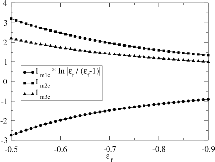
FIG. 2.: Contributions to the occupied-state selfenergy from the Coulomb correction to the effective hybridization vertex: Occupied-state integrals $I_{mic}(\epsilon_{f})$ evaluated for various values of the f-level energy $\epsilon_{f}$. Here and in all further Figures solid lines are guides for the eye.

The spin fluctuations integrals are of analogical properties but for $\omega<\omega_{0}$. The infinitesimal imaginary parts $+i0_{+}$ in denominators of the integrands in Eqs. (62-72) are omitted because they do not contribute for $\omega<\epsilon_{f}$. Note that for $n_{f}<1$ integrals $I_{0ic}$, $I_{0is}$ have to be inserted in Eq.(59) being multiplied by $n_{f}$ or $1-n_{f}$ correspondingly. The contributions from the spin fluctuations to the Coulomb renormalization of the occupied-state vertex $I_{misf}$ are neglected. The Coulomb contributions to the occupied-state selfenergy vary rather smoothly with $\omega$ in the vicinity of $\epsilon_{f}$.

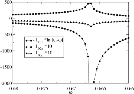
FIG. 3.: Charge fluctuation contribution to empty-state selfenergy integrals $I_{0ic}(\omega)$ for $\epsilon_{f}=-2/3$, $\Delta=0.2$, $U=0.1$ For $\omega>\epsilon_{f}$ the real part is shown.

They give rise to a rather small shift of the effective f-level which can be estimated from the integrals $I_{mic}(\epsilon_{f})$ displayed in Figure 2 and the real part of the selfenergy $\Sigma_{m}^{(U)}(\epsilon_{f})$. As we shall see below, we need not explicitly account for the shift in the determination of the many-body low-energy scale.

Let us now turn to the empty state selfenergy. Following the iterative procedure we include the charge fluctuations in the first step. The variation with energy of the integrals $I_{0ic}(\omega)$ is displayed in Figure 3.

A detailed analysis shows that in the energy range of interest the integrals vary approximately like $I_{01c}(\omega)\sim A_{1}\ln|\omega-\epsilon_{f}|+B_{1}$ and $I_{02c}(\omega)\sim(A_{2}\ln|\omega-\epsilon_{f}|+B_{2})^{2}$ where $A_{1}>A_{2}$. The resulting real part of the empty-f state self-energy varies like $-(\log|\epsilon_{f}-\omega|)^{2}$ in the vicinity of the (renormalized) f-level. As a consequence, the corresponding Green’s function $G_{0}(\omega)$ always exhibits a pole at $\omega_{0}(U)<\omega_{0}(U=0)<\epsilon_{f}$. For not too small values of the hybridization width they are well described by the linear dependence

$$\omega_{0}(U)\simeq\omega_{0}(U=0)+\frac{\displaystyle\Re\Sigma_{0c}^{(U)}(\omega_{0})}{\displaystyle 1-\left[\frac{\partial\Re\Sigma_{0}^{(0)}(\omega)}{\partial\omega}\right]}_{\omega_{0}}$$ (73)

The change in the pole is seen to be proportional to the weight of the f⁰-configuration in the ground state times the Coulomb repulsion among the conduction electrons.

For a first qualitative understanding of the variation with the Coulomb repulsion of the threshold energy $\omega_{0}$ one may use ”on-shell” approximation [20]. Within this approximation, the empty-state selfenergy $\Sigma_{0}(\omega)=\frac{2{\tilde{\Delta}}}{\pi}\ln\left[{\tilde{\epsilon}}_{f}-\omega\right]$ has the same $\omega$- dependence as in the non-interacting case but with renormalized parameters: ${\tilde{\Delta}}=\Delta\left(1-\frac{U}{4\pi}\Delta I_{01c}\left(\omega_{0}\right)\right);{\tilde{\epsilon}}_{f}=\epsilon_{f}-\frac{U\Delta^{2}}{2\pi^{2}}\left(I_{02c}\left(\omega_{0}\right)+I_{03c}\left(\omega_{0}\right)\right)$ with $\omega_{0}=\omega_{0}(U=0)$ here. We see that ${\tilde{\Delta}}>\Delta$ and $|{\tilde{\epsilon}}_{f}|>|\epsilon_{f}|$. If the impurity valence is close to integer which lead to a Kondo regime the renormalization of the hybridization coupling prevails the renormalization of the f-level energy resulting in an effective enhancement of the Kondo energy scale. The simplified approach, however, cannot be used for quantitative estimates. Unfortunately the variation with $U$ of the corresponding Kondo-type pole is systematically underestimated ( $T_{K}$ is overestimated ) as can be easily seen from the slopes

$\frac{\partial\omega_{0}^{OnShell}}{\partial U}-\frac{\partial\omega_{0}}{\partial U}=-\frac{1}{2\pi^{2}}\Delta^{2}\left(I_{02c}(\omega_{0})+I_{03c}(\omega_{0})\right)<0$

The results for the Kondo pole change only slightly upon iteration. Inclusion of the spin fluctuation contribution to the Coulomb correction yields a rather small shift in the selfenergy which further stabilizes the Kondo ground state. This can be seen from the calculated variation with energy of the integrals $I_{0isf}(\omega)$. The full selfenergy $\Sigma_{0}(\omega)$ is shown in Figure 4.

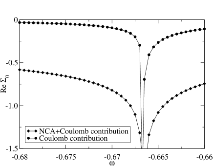
FIG. 4.: Variation with energy of the real part of the full empty-state selfenergy $\Re\Sigma_{0}^{(U)}(\omega)$ from NCA plus Coulomb correction to the hybridization vertex for $\epsilon_{f}=-2/3$, $\Delta=0.2$ and $U=0.1$

The characteristic energy scale for low-energy excitations, i. e., the Kondo temperature, is now calculated as the difference between the ground state energy - the threshold $\omega_{0}$ - and the energy of the f-level $\epsilon_{f}$

$$k_{B}T_{K}=\epsilon_{f}-\omega_{0}$$ (74)

At this point we should like to add a comment concerning the choice of $\epsilon_{f}$. This quantity enters Eq. (74) explicitly as well as implicitly through $\omega_{0}$. If we were to account for the Coulomb renormalization we would have to do it consistently. This means we would have to consider the difference

$\epsilon_{f}+\delta\epsilon_{f}-\omega_{0}(\epsilon_{f}+\delta\epsilon_{f})\simeq\epsilon_{f}-\omega_{0}+\delta\epsilon_{f}\left(1-n_{f}\right)$. The correction from the Coulomb contribution is hence proportional to $\delta\epsilon_{f}\left(1-n_{f}\right)$ which is rather small in our case because the shift $\Re\Sigma_{m}(\omega)$ is very small.

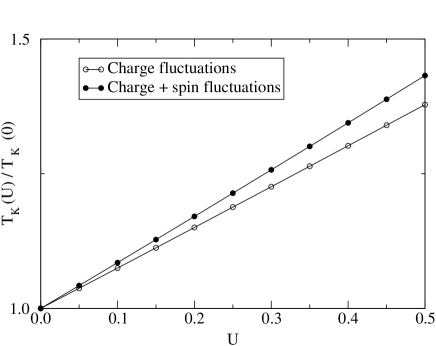
FIG. 5.: Enhancement of the Kondo temperature for $\epsilon_{f}=-2/3$ and $\Delta=0.2$. Charge fluctuations are dominant.

To conclude, we can calculate $k_{B}T_{K}$ from Eq. (74) using the the bare f-level energy at $\epsilon_{f}$. The results displayed in Figure 5 show the enhancement of the Kondo temperature due to the Coulomb interaction among the conduction electrons.

Following up the iteration procedure the spectral function

$$A_{0}(\omega)=-\frac{1}{\pi}\Im\left(\omega-\Sigma_{0}^{(0)}-\Sigma_{0c}^{(U)}\right)^{-1}$$ (75)

is inserted in to Eq. (59). It comes from calcultions that including the spin fluctuation peak at $\omega=\omega_{0}(U)$ does not significantly alter the empty-state selfenergy $\Sigma_{0}^{(U)}(\omega)$ in the Kondo regime. The spin fluctuations lower the energy of the pole in the Green’s function $G_{0}(\omega)$ and therefore further stabilize the Kondo ground state. This can be seen from Figure 5. The data suggest the charge fluctuation contribution already gives a rather good estimate of the Coulomb correction to the low-temperature properties to leading order in the inverse degeneracy.

The main feature of the above caculations is the factorization of the ‘NCA-bubble’ self-energy $\Sigma_{0}^{0}(\omega)$ in the r.h.s. of Eq. (59) for the empty state self-energy $\Sigma_{0}^{(U)}(\omega)$. This factorisation is due to the possibility, as it was shown for the orbital degeneracy case in Appendix A, to neglect the momentum conservation in the integrals of the $V^{(4)}$ coupling, Eq. (18). Therefore results of this section are also valid for the degenerate case if one replace in Eq. (59) $\Delta\rightarrow(N-1)\Delta$. So the renormalisation of the paramerers of the Anderson impurity Hamiltonian is selfconsistent, in the spirit of the NCA.

V Thermodynamic properties at Zero Temperature

The results of the preceeding section allow us to assess the influence of the conduction electron Coulomb repulsion on the thermodynamic properties of dilute magnetic alloys. Of particular interest are the low-temperature f-valence $n_{f}$, the $f$-charge susceptibility $\chi_{c}$, the $f$-spin susceptibility $\chi_{s}$ and the magnetic contribution to the linear coefficient of the specific heat $\gamma$. Previous calculations based on the symmetric Anderson model yield a rather strong depression with U of the $f$ magnetic susceptibility [14]. Data for the U-dependence of the f valence $n_{f}$ and the f charge susceptibility $\chi_{c}$, however could not be obtained from these model studies since particle-hole symmetry pins $n_{f}$ to unity. For a first quantitative estimate we approximate the empty-state selfenergy $\Sigma_{0}$ by

$$\Sigma_{0}^{(0)}\rightarrow\Sigma_{0}^{(0)}+\Sigma_{0c}^{(U)}$$ (76)

keeping only the charge fluctuation contribution. This procedure should be justified in the Kondo limit where the deviation from integer f valence is small. The pole of the corresponding Green’s function, $\omega_{0}$, can be interpreted as the ground state of the system. It yields the dominant low-temperature contribution to the partition function, and the thermodynamic properties follow by straightforward differentiation [6]

$$n_{f} = \frac{\partial\omega_{0}}{\partial\epsilon_{f}}$$ (77)

$$\chi_{c} = -\frac{\partial^{2}\omega_{0}}{\partial\epsilon_{f}^{2}}$$ (78)

$$\chi = \lim_{H\to 0}\left(-\frac{\partial^{2}\omega_{0}}{\partial H^{2}}\right)$$ (79)

$$\gamma = \lim_{T\to 0}\left(-\frac{1}{T}\frac{\partial\omega_{0}(T)}{\partial T}\right)$$ (80)

Finally, we shall discuss the Sommerfeld-Wilson ratio $R$, i. e. , the ratio of the zero-temperature spin susceptibility and the specific heat coefficient

$$R=\frac{\displaystyle\frac{\pi^{2}}{3}\chi}{\displaystyle\frac{\mu_{j}^{2}}{3}\gamma}$$ (81)

where $\mu_{j}^{2}=j(j+1)(g\mu_{B})^{2}$.

Our main interest is in the linear in U corrections to the experimental quantities. These contributions can be easily obtained from the linear in U corrections to the ground state energy as given by Eq. (73). We specify the interaction related enhancement/reduction in terms of the coefficients

$$n_{f}(U) \simeq n_{f}^{(0)}\left(1+Un_{f}^{(1)}\right)$$ (82)

$$\chi_{c}(U) \simeq \chi_{c}^{(0)}\left(1+U\chi_{c}^{(1)}\right)$$ (83)

$$\chi_{s}(U) \simeq \chi_{s}^{(0)}\left(1+U\chi_{s}^{(1)}\right)$$ (84)

$$\gamma_{f}(U) \simeq \gamma_{f}^{(0)}\left(1+U\gamma_{f}^{(1)}\right)$$ (85)

$$R(U) \simeq R^{(0)}\left(1+UR^{(1)}\right)$$ (86)

which depend upon the f-level position $\epsilon_{f}$ and the hybridization width $\Delta$ and, concomitantly, on the Kondo energy $k_{B}T_{K}^{(0)}$ of the reference system with non-interacting conduction electrons.

The explicit evaluation requires the generalization of $\Sigma_{0}^{(U)}$ to low but finite temperatures and to small external magnetic fields. The former is easily achieved by starting from Eq. (53) and proceeding in close analogy to the zero temperature case keeping the Fermi functions instead of the step functions. The derivatives with respect to temperature are calculated from a Sommerfeld expansion. An external magnetic field, on the other hand, lifts the the degeneracy of the f-level according to [37]

$$\epsilon_{f}\longrightarrow\epsilon_{f}+\sigma h\quad.$$ (87)

The NCA contribution $\Sigma_{0}(\omega)=\frac{\Delta}{\pi}\sum_{\sigma}\ln\left[\epsilon_{f}+\sigma h-\omega\right]$ is directly read off. The Coulomb contribution is now expressed in terms of three spin-dependent integrals $I_{0i}(\omega;\sigma)$ which which closely parallel their counterparts in the absence of an external magnetic field $I_{0i}(\omega)$. Keeping only the charge fluctuation contribution yields

$$\Sigma_{0}^{(U)}\left(\omega\right) = \sum_{\sigma}\frac{1}{{\bf 4\pi^{2}}}U\Delta^{2}\left(-I_{01}(\omega;\sigma)\ln\left|{\epsilon_{f}-\sigma h-\omega}\right|+I_{02}(\omega;\sigma)+I_{03}(\omega;\sigma)\right)$$ (88)

$$I_{01c}(\omega;\sigma) = \int_{0}^{1}\!\!dx\!\!\int_{0}^{1}\!\!dy\,\frac{2}{(-\omega\!+\!x\!+\!y)(-\omega\!+\!\epsilon_{f}\!+\sigma h\!+\!x)}\ln\left[\frac{-\omega\!+\!\epsilon_{f}\!-\sigma h\!+\!x\!+\!y}{-\omega\!+\!\epsilon_{f}\!-\sigma h\!+\!x\!+\!y\!+1}\right]$$ (89)

$$I_{02c}(\omega;\sigma) = \tilde{I}_{02c}(\omega;\sigma)\tilde{I}(\omega;-\sigma)$$ (90)

$$\tilde{I}_{02c}(\omega;\sigma) = \int_{0}^{1}\!\!dx\!\!\,\frac{1}{(-\omega\!+\!\epsilon_{f}+\!\sigma h+\!x)}\ln\left[\frac{-\omega+1+x}{-\omega+x}\right]$$ (91)

$$I_{03c}(\omega;\sigma) = \int_{0}^{1}\!\!dx\!\!\int_{0}^{1}\!\!dy\!\!\int_{0}^{1}\!\!dz\frac{2\ln\left[\frac{x+y+z+1}{x+y+z}\right]}{(-\omega\!+\!x\!+\!y)(-\omega\!+\!\epsilon_{f}\!+\!\sigma h\!+\!x)(-\omega\!+\!\epsilon_{f}\!-\!\sigma h\!+\!x\!+\!y\!+\!z)}\quad.$$ (92)

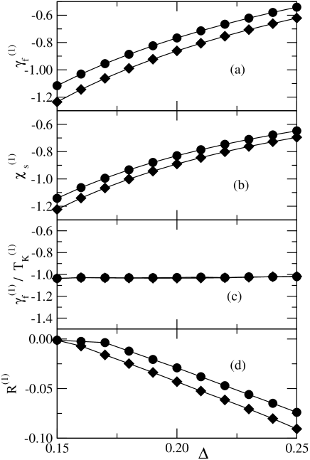
FIG. 6.: Reduced thermodynamical coefficients from Eq. 86 as functions of $\Delta$ for $\epsilon_{f}=-2/3$ (diamonds) and $\epsilon_{f}=-0.7$ (circles). (a):${\bar{\gamma}}_{f}^{(1)}$, (b):${\bar{\chi}}_{s}^{(1)}$, (c):${\bar{\gamma}}_{f}^{(1)}{\bar{T}_{K}^{(1)}}$, (d):${\bar{R}}^{(1)}$

At low temperatures, we find a finite temperature-independent Pauli-like spin susceptibility and a linear specific heat indicating a nonmagnetic Fermi liquid ground state. The results are displayed in Figure 6(a) and (b). The coefficient $\gamma_{f}$ of the linear specific heat is reduced by the conduction electron interactions reflecting the enhancement of the Kondo temperature. The scaling $\gamma_{f}\sim 1/T_{K}$ can be seen from from Figure 6(c)[39]. Similarly, the magnetic susceptibility is reduced by the conduction electron interactions. The reduction determined here is comparable to the value obtained by Hofstetter et al. [14]. Its actual values, however, exhibit deviations from universal scaling with the inverse Kondo temperature $1/T_{K}$ reflecting the importance of quasiparticle interactions. This is to be expected from the explicit expression for the spin susceptibility calculated to leading order in the conduction electron interaction

$$\chi_{s}(U)/\chi_{s}^{(0)}\simeq 1-\left[\frac{\partial}{\partial\omega}\log\left(-\frac{\frac{\partial^{2}\Sigma_{0}^{(0)}}{\partial h^{2}}}{1-\frac{\partial\Sigma_{0}^{(0)}}{\partial\omega}}\right)\right]_{\omega_{0}^{(0)},h=0}\delta T_{K}$$ (93)

$$+\left(\left[\frac{\frac{\partial\Sigma_{0}^{(U)}}{\partial\omega}}{1-\frac{\partial\Sigma_{0}^{(0)}}{\partial\omega}}\right]_{\omega_{0}^{(0)},h=0}+\left[\frac{\frac{\partial^{2}\Sigma_{0}^{(U)}}{\partial h^{2}}}{\frac{\partial^{2}\Sigma_{0}^{(0)}}{\partial h^{2}}}\right]_{\omega_{0}^{(0)},h=0}\right)\quad$$ (94)

The interaction correction to the spin susceptibility consists of two terms where the first one is proportional to the change in the Kondo temperature. As its coefficient varies proportional to $T_{K}(0)^{-2}$ we expect this contribution to dominate in the close to integer valence limit where $T_{K}(0)$ becomes small. In this limit we should recover the typical Kondo scaling. The second term which results from the variation with h of the interaction corrections tends to further reduce the spin susceptibility. Within the spirit of Landau’s Fermi liquid theory it gives rise to a positive Landau parameter $F_{0}^{(a)}$.

The deviation from simple scaling is also reflected in the Sommerfeld-Wilson ratio which is reduced by the conduction electron Coulomb interaction (see Figure 6(d)). Since

$${\bar{R}}^{(1)}\simeq{\bar{\chi}}_{s}^{(1)}-{\bar{\gamma}}_{f}^{(1)}.$$ (95)

this quantity allows us to estimate the Landau parameter ${\bar{R}}^{(1)}\simeq-F_{0}^{(a)}$.

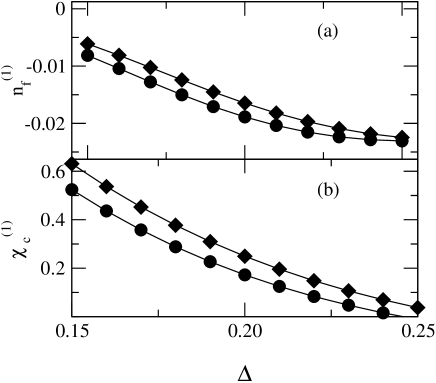
FIG. 7.: Reduced thermodinamical coefficients from Eq. 86 as functions of $\Delta$ for $\epsilon_{f}=-2/3$ (diamonds) and $\epsilon_{f}=-0.7$ (circles). (a):${\bar{n}}_{f}^{(1)}$, (b):${\bar{\chi}}_{c}^{(1)}$

The deviations from the universal scaling with $T_{K}$ are most strongly evident in the f-valence, $n_{f}$, and in the f-charge susceptibility, $\chi_{c}$ displayed in Figure 7. The f-valence is slightly decreased by the conduction electron Coulomb repulsion as can be seen from the coefficient ${\bar{n}}_{f}^{(1)}$ displayed in Figure 7, (a). This behavior reflects two competing effects, i. e., (a) the increase in characteristic energy as demonstrated in Figure 5 which is partially compensated by (b) the enhancement of the effective hybridization.

The f-charge susceptibility $\chi_{c}$ is affected more dramatically as suggested by the coefficient ${\bar{\chi}}_{c}^{(1)}$ in Figure 7, (b). In the Kondo regime, it is enhanced by the Coulomb interaction of the conduction electrons. This enhancement, however, decreases as we approach the mixed-valent regime. In this parameter regime, however, the adopted approximation (charge fluctuation contribution to selfenergy only) ceases to be valid.

To summarize, the low-temperature properties of a dilute magnetic alloy are significantly modified by the Coulomb repulsion of the conduction electrons. The local Fermi liquid properties are preserved in the sense that the magnetic contribution to the specific heat varies linearly with temperature, $C_{f}\sim T$, and that the magnetic susceptibility $\chi_{s}$ is finite at $T=0$. Even in the lowest order in the inverse degeneracy, the low-temperature properties are not universal in the sense that their variation with U cannot be accounted for by properly adjusting the Kondo temperature.

VI Discussions

We formulated here the NCA equations for an Anderson impurity coupled to interacting conduction electrons. Due to the CEI an energy-dependent effective hybridization vertex appears in the usual NCA equations. The case of weak CEI was investigated in detail here including calculations of measurable thermodynamical properties of a dilute magnetic impurities system. The results for a rigid, i. e., energy-independent vertex can serve as a guide-line for the case of a magnetic impurity embedded in a Fermi liquid where the central quantity is the quasiparticle t-matrix [40].

For weak electron-electron interaction the increase of $T_{K}$ may be understood as resulting from the reduced probability of finding doubly occupied and empty lattice sites in the correlated conduction electron systems. The increased number of uncompensated conduction electron spins finally leads to the enhancement of the effective hybridization coupling. The analogy between the Kondo spin model and the Anderson impurity model in its local moment regime is not complete in the case of correlated conduction electrons ( see also [17] ). In the former case $T_{K}$ will increase monotonously with $U$ because of the enhancement of the exchange interaction. In the latter case the process is two-staged, it involves the formation of a local moment and its interaction with the conduction electrons. As we show here CEI influence thermodynamical quantities in a non-trivial fashion: the specific heat coefficient $\gamma(U)$ scales with $T_{K}(U)$ like in the non-interacting case while the magnetic susceptibility $\chi_{s}(U)$ does not. That may be understood because the latter quantity depends not only on the low energy excitations spectrum as the former but also on the matrix element which is influenced by CEI.

There is some controversy about the scaling with $T_{K}(U)$ of $\chi_{s}(U)$. In a somewhat artificial model of [16] the scaling of $\chi_{s}(U)$ with $T_{K}(U)$ is preserved for not too large values of $U$. In the paper [14] this question is not discussed explicitly but it may be judged from the relevant plots in [14] that their results do not show the usual scaling behaviour of $\chi_{s}(U)$ but rather resemble our results.

The present results are based on the separation of energy scales. In so far as the vertex correction does not produce a new low frequency scale or does not dominatly contribute to the empry state ( empty-f-state ) self-energy we anticipate no qualitative changes when using more sophisticated approximations for the vertices $\Gamma_{\sigma,\bar{\sigma}}^{\left(U\right)}\left(1,2;3,4\right)$, (Figure 1 c) appropriate for the strong correlation regime. We may expect that for sufficiently large $U$ the virtual transition from the f-state to the conduction state will cost too much energy inhibiting the $T_{K}$-increase and leading eventually to the change in the trend [13, 14]. For a quantitative treatment of this problem there are two visible approaches. One is to introduce summation of the infinite subseries of the ring, the ladder and the particle-particle type starting with the 2nd order self-energies [32]. The other way is to approximate the vertex correction by response functions ( dynamic susceptibilities ). The other visible development of the theory of the Kondo effect for electronic correlated system in general and high-$T_{c}$ cuprates in particular is the use of the antiferromagnon dynamic susceptibility [41] or other phenomenological models which develop a short-range order with the virtual breaking of singlet-triplet degeneracy in the conduction-electron system ( see also Ref. [13] ). In addition, the influence of conduction electron interactions on the spectral properties of magnetic impurities and their dependence upon the doping are also interesting topics for future investigations.

In conclusion, the NCA theory of an Anderson impurity embedded in a metall with correlated conduction electrons is developed and general NCA equations for the interacting conduction electrons are obtained. It is shown that due to the renormalisation of the hybridization interaction the characteristic energy is increased by the weak interactions. The influence of weak conduction electron interations on thermodynamic properties of magnetic impurities is discussed.

VII Acknowledgments

The hospitality at TU-Braunschweig is acknowledged by V.Z. This work was supported by the Niedersächsisch-Israelischer Foundation. Discussions with Dr. A. Schiller are appreciated.

A Fourth order term

We estimate the variation with the orbital degeneracy $N$ of the vertex-corrected boson selfenergy (Figure 1(c) assuming a simple band structure for the metallic host. The orbitally degenerate conduction bands are modelled by tight-binding s-bands the dispersion being determined by hoping between nearest neighbor sites on a simple cubic lattice. The magnetic impurity sitting at the origin is surrounded by six nearest neighbors. The wave vector dependence of the coupling between the conduction states and the strongly correlated local orbital $(j,m)$ is given by the canonical structure constant $S_{00;jm}(\vec{k})$ [42, 43] of the Atomic Sphere Approximation (ASA) to the Linear Muffin Tin Orbital (LMTO) method. Here $j$ and $m$ refer to the azimuthal and magnetic quantum number of the impurity orbital under consideration.

Let us neglect spin-orbit interaction for a first qualitative discussion. The hybridization matrix element $V_{m\sigma}(\vec{k})$ does not depend upon $\sigma$. It is given by

$$V_{m\sigma}(\vec{k})=V_{0}({\epsilon_{\vec{k}}})\sum_{\vec{R}_{j}}e^{i\vec{k}\cdot\vec{R}_{j}}\left[\sqrt{4\pi}iY_{\ell m}(\hat{R}_{j})\right]^{*}\left(\frac{S}{\left|\vec{R}_{j}\right|}\right)^{\ell+1}$$ (A1)

where the argument $\hat{R}_{j}$ of the spherical harmonic $Y_{\ell m}$ denotes the unit vector pointing from the impurity to the nearest neighbor sites $\vec{R}_{j}$. The overall length scale $S$ is usually chosen as the average atomic radius while $V_{0}(\epsilon_{\vec{k}})$ is an energy-dependent real prefactor.

Starting from this form of the hybridization we shall first derive an expression for the second order term which is subsequently compared to the fourth order average.

The sum

$$\sum_{m}V_{m\sigma}^{*}(\vec{k})V_{m\sigma}(\vec{k}^{\prime})$$ (A2)

is easily evaluated using the addition theorem for spherical harmonics

$$\sum_{m_{-}\ell}^{\ell}\left(Y_{\ell m}(\hat{R}_{j})\right)^{*}Y_{\ell m}(\hat{R}_{j^{\prime}})=\frac{2\ell+1}{4\pi}P_{\ell}\left(\hat{R}_{j}\cdot\hat{R}_{j^{\prime}}\right)=$$ (A3)

$$\frac{N}{4\pi}P_{\ell}\left(\hat{R}_{j}\cdot\hat{R}_{j^{\prime}}\right)$$ (A4)

where $N=2\ell+1$ is the degeneracy of the impurity level. For a simple cubic lattice with

$$\hat{R}_{j}\cdot\hat{R}_{j^{\prime}}=\delta_{\hat{R}_{j}\hat{R}_{j^{\prime}}}-\delta_{\hat{R}_{j},-\hat{R}_{j^{\prime}}}$$ (A5)

we obtain for $\ell=3$

$$\sum_{m}V_{m\sigma}^{*}(\vec{k})V_{m\sigma}(\vec{k}^{\prime})V_{0}(\epsilon_{\vec{k}})V_{0}(\epsilon_{\vec{k}^{\prime}})N\times$$ (A6)

$$\sum\,\,_{\vec{R}_{j}}\left(e^{-i\vec{k}\cdot\vec{R}_{j}}e^{i\vec{k}^{\prime}\cdot\vec{R}_{j}}-e^{-i\vec{k}\cdot\vec{R}_{j}}e^{-i\vec{k}^{\prime}\cdot\vec{R}_{j}}\right)\quad.$$ (A7)

As expected, the second order term entering the non-crossing diagram

$$\langle\sum_{m}\left|V_{m\sigma}(\vec{k})\right|^{2}\rangle_{\epsilon} = \left|V_{0}(\epsilon)\right|^{2}N\langle\sum\,\,_{\vec{R}_{j}}\left(1-\cos 2\vec{k}\cdot\vec{R}_{j}\right)\rangle_{\epsilon}$$ (A8)

$$= \left|V_{0}(\epsilon)\right|^{2}N2\langle\sum\,\,_{\vec{R}_{j}}\sin^{2}\vec{k}\cdot\vec{R}_{j}\rangle_{\epsilon}$$ (A9)

$$= \left|V_{0}(\epsilon)\right|^{2}2zN\langle\sin^{2}k_{x}\rangle_{\epsilon}$$ (A10)

is proportional to the degeneracy $N=2\ell+1$ and the number of nearest neighbbors with $z=6$ for s.c.l.. The average over the constant energy surface which has to be numerically evaluated is of order unity and varies smoothly with the energy $\epsilon$. To summarize: The non-crossing diagrams involve the combination

$$N\Delta(\epsilon)=NN(\epsilon)\left|V_{0}(\epsilon)\right|^{2}2z\langle sin^{2}k_{x}\rangle_{\epsilon}$$ (A11)

The contributions from the Coulomb-corrected vertex, on the other hand, require the fourth-order term from Eq. (18):

$$\sum_{m}V_{m}^{(4)}(E_{1},E_{2},E_{3},E_{4})=\frac{1}{L^{3}}\sum_{\vec{k}_{1},\vec{k}_{2},\vec{k}_{3},\vec{k}_{4}}$$ (A12)

$$\delta(\epsilon_{\vec{k}_{1}}-E_{1})\delta(\epsilon_{\vec{k}_{2}}-E_{2})\delta(\epsilon_{\vec{k}_{3}}-E_{3})\delta(\epsilon_{\vec{k}_{4}}-E_{4})\times$$ (A13)

$$\sum_{m,m^{\prime}}V_{m\sigma_{1}}(\vec{k}_{1})V_{m\sigma_{3}}^{*}(\vec{k}_{3})\sum_{m^{\prime}}V_{m^{\prime}\sigma_{2}}(\vec{k}_{2})V_{m^{\prime}\sigma_{4}}^{*}(\vec{k}_{4})\times$$ (A14)

$$\delta^{*}(\vec{k}_{1}+\vec{k}_{2}-\vec{k}_{3}-\vec{k}_{4})$$ (A15)

where $\delta^{*}(\vec{k}_{1}+\vec{k}_{2}-\vec{k}_{3}-\vec{k}_{4})$ is the Laue function, Eq. (19). If we were to neglect momentum conservation this expression would vanish identically.

Inserting the explicit expressions for the hybridization matrix elements Eq. (A1) reduces to a sum of local contributions

$$\sum_{m}V_{m}^{(4)}(E_{1},E_{2},E_{3},E_{4})=\sum_{\vec{R}_{n}}\sum_{m,m^{\prime}}I_{m\sigma_{1}}(\vec{R}_{n},E_{1})\times$$ (A16)

$$I_{m^{\prime}\sigma_{2}}(\vec{R}_{n},E_{2})I_{m\sigma_{3}}^{*}(\vec{R}_{n},E_{3})I_{m^{\prime}\sigma_{4}}^{*}(\vec{R}_{n},E_{4})$$ (A17)

where the averages

$$I_{m\sigma}(\vec{R}_{n},E)=N(E)\langle V_{m\sigma}(\vec{k})e^{i\vec{k}\cdot\vec{R}_{n}}\rangle_{E}$$ (A18)

are given by

$$I_{m\sigma}(\vec{R}_{n},E)=N(E)V_{0}(E)\left(-i\right)\sqrt{4\pi}\sum_{\vec{R}_{j}}Y_{3m}^{*}\left(\hat{R}_{j}\right)$$ (A19)

$$\langle e^{i\vec{k}\cdot\vec{R}_{j}}e^{i\vec{k}\cdot\vec{R}_{n}}\rangle_{E}\quad.$$ (A20)

In the next step, we sum over the magnetic quantum numbers $m$ and $m^{\prime}$

$$\sum_{m=-\ell}^{\ell}I_{m\sigma_{1}}(\vec{R}_{n},E_{1})I_{m\sigma_{3}}^{*}(\vec{R}_{n},E_{3})$$ (A21)

$$= V_{0}(E_{1})V_{0}(E_{3})\sum_{\vec{R}_{j},\vec{R}_{j}^{\prime}}\langle e^{i\vec{k}_{1}\cdot\left(\vec{R}_{j}+\vec{R}_{n}\right)}\rangle_{E_{1}}\langle e^{-i\vec{k}_{3}\cdot\left(\vec{R}_{j^{\prime}}+\vec{R}_{n}\right)}\rangle_{E_{3}}$$ (A22)

$$\times 4\pi\sum_{m=-\ell}^{\ell}Y_{3m}^{*}\left(\hat{\vec{R}}_{j}\right)Y_{3m}^{*}\left(\hat{\vec{R}}_{j^{\prime}}\right)$$ (A23)

$$= NV_{0}(E_{1})V_{0}(E_{3})\sum_{\vec{R}_{j}\neq 0}\langle e^{i\vec{k}_{1}\cdot\left(\vec{R}_{j}+\vec{R}_{n}\right)}\rangle_{E_{1}}$$ (A24)

$$\times \langle\left(e^{-i\vec{k}_{3}\cdot\vec{R}_{j})}-e^{i\vec{k}_{3}\cdot\vec{R}_{j}}\right)e^{-i\vec{k}_{3}\cdot\vec{R}_{n})}\rangle_{E_{3}}$$ (A25)

The local term $\vec{R}_{j}$ vanishes identically due to the symmetry of the constant energy surface. For finite $\vec{R}_{n}$, the averages over the constant energy surfaces decay with increasing $\vec{R}_{n}$ due to the oscillatory behavior of the integrand. The leading contribution to the lattice sum involves the nearest neighbor term, e. g. $\vec{R}_{n}=(1,0,0)$. In the subsequent summation over the nearest neighbors $\vec{R}_{j}$, the nonvanishing contributions are given by $\vec{R}_{j}=(-1,0,0)$ and $\vec{R}_{j}=(1,0,0)$ yielding

$$\langle 1-\cos 2k_{x}\rangle_{E_{1}}\langle 1-\cos 2k_{x}\rangle_{E_{2}}=4\langle\sin^{2}k_{x}\rangle_{E_{1}}\langle\sin^{2}k_{x}\rangle_{E_{2}}\quad.$$ (A26)

The leading contribution to the fourth-order term $V^{(4)}$ hence factorizes according to

$$\frac{1}{N}\sum_{m}V^{(4)}(E_{1},E_{2},E_{3},E_{4})=$$ (A27)

$$zN\prod_{r=1}^{4}N(E_{r})V_{0}(E_{r})2\langle\sin^{2}k_{x}\rangle_{E_{r}}$$ (A28)

The average $2\langle\sin^{2}k_{x}\rangle_{E}$ is of order unity as mentioned above. If we neglect the dependence of the density of states and $V_{0}$ on the energy $E$ we find for the averaged value of $V^{(4)}(E_{1},E_{2},E_{3},E_{4})$

$$V^{(4)}=\frac{N}{z}\left(\frac{N(\epsilon_{f})\Delta}{\pi}\right)^{2}$$ (A29)

In conclusion, we showed that in the leading approximation of the hybridisation matrix element expansion, Eq. (A1), the ratio $\frac{V^{(4)}}{(\Delta N(\epsilon_{f})/\pi)^{2}}\simeq\frac{N}{z}$ i.e. of the order of unity.

REFERENCES

- [1] Present address: Institute for Bioinformatics, German National Center for Health and Environment, Ingolstädter Landstra e 1, 85764 Neuherbeg, Germany
- [2] A. M. Tsvelick and P. B. Wiegmann, Adv. Phys. 32, 453 (1983).
- [3] N. Andrei, K.Furuya and J. H.Lowenstein, Rev. Mod. Phys. 55, 331 (1983).
- [4] P. Fulde, J. Keller, and G. Zwicknagl, in Solid State Physics, edited by F. Seitz, D. Turnbull, and H. Ehrenreich (Academic Press, New York, 1988), Vol. 41, p. 1.
- [5] G. Zwicknagl, Adv. Phys. 41, 203 (1992).
- [6] A. C. Hewson, The Kondo Problem to Heavy Fermions (Cambridge University Press, Cambridge, 1993).
- [7] D. H. Lee and J. Toner, Phys. Rev. Lett. 69, 3378 (1992).
- [8] A. Furusaki and N. Nagaosa, Phys. Rev. Lett. 72, 892 (1994).
- [9] A. Schiller and K. Ingersent, Phys. Rev. Lett. 51, 4676 (1995).
- [10] Y. M. Li, Phys. Rev . B 52, R6979 (1995).
- [11] P. Phillips and N. Sandler, Phys. Rev. B 53, 468 (1996).
- [12] A. Schiller and K. Ingersent, Europhys. Lett. 39, 645 (1997).
- [13] B. Davidovich and V. Zevin, Phys. Rev. B 57, 7773 (1998).
- [14] W. Hofstetter, R. Bulla, and D. Vollhardt, Phys. Rev. Lett. 84, 4417 (2000).
- [15] W. K. A. Georges, G. Kotliar, W. Krauth, and M. J. Rozenberg, Rev. Mod. Phys. 68, 13 (1996).
- [16] R. Takayama, O.Sakai, Jour. Phys. Soc. Jap., 67, 1844 (1998).
- [17] G. Khaliullin and P. Fulde, Phys. Rev. B 52, 9514 (1995).
- [18] T. Schork, Phys. Rev. B 53, 5626 (1996).
- [19] K. Itai and P. Fazekas, Phys. Rev. B 54, R752 (1996).
- [20] S. Tornow, V. Zevin, and G. Zwicknagl, cond-mat 9701137 (1997).
- [21] T. A. Costi and A. Newns, Physica C 185-189, 2649 (1991).
- [22] R. Takayama and O. Sakai, Physica B 186-188, 915 (1993).
- [23] I.E.Perakis, C. M. Varma, and A. E. Ruckenstein, Phys. Rev. Lett. 70, 3467 (1993).
- [24] T. Giamarchi, Phys. Rev. Lett. 70, 3967 (1993).
- [25] J. K. A. Bauer, Z. Phys. B 96, 383 (1995).
- [26] The non-degenerate case may evolve from the orbital degenerate case as the consequence of the crystal electric field splitting.
- [27] N. E. Bickers, RMP 59, 845 (1987).
- [28] A. Bringer and H. Lustfeld, Z. Phys.. B 28, 213 (1977).
- [29] P. Fulde, Electron Correlations in Molecules and Solids, 3rd ed. (Springer Verlag, Berlin, 1995), and references therein.
- [30] P. Fazekas, Electron Correlations and Magnetism (World Scientific, Singapore, 1999), and references therein.
- [31] P. Coleman, Phys. Rev. B 53, 271 (1983).
- [32] S. Tornow, Ph.D. thesis, U Stuttgart, 1997.
- [33] J. Hubbard, Proc. R. Soc. London. A 281, 401 (1964).
- [34] L. Roth, Phys. Rev. 184, 451 (1969).
- [35] Both the degenerate ( ) and the non-degenerate cases are considered. In the case of the non-degenerate Anderson impurity index consides with the electron spin index and the coupling does not depend ( in a paramagnetic host and by neglecting the spin-orbit interaction ) on the spin orientation. So in the non-degenerate Anderson impurity case the subscript m coincides with and .
- [36] As it is known from the NCA-method, Eq. (57) is the first step in the NCA iteration procedure ( see [27] ) which already captures right the exponent of the Kondo energetic scale.
- [37] One has have in mind that Eq. (87) is strictly speaking applyed for the bubble of Figure 1, a. For Figure 1, c changes sign ‘across’ interaction .
- [38] The generalization on other filling is trivial [18]. Our integral functions , i =1, 2, 3, are very close to analogical integrals in ref. [18], , and correspondingly.
- [39] In Figure 6(c) we use which is defined in close analogy to the thermodynamical parameters as . The value of is obtained in a straightforward way from Eqs. (74), (73). Then from the scaling follows .
- [40] The influence of residual interactions of Fermi liquid quasiparticles on the Kondo effect may be interesting for the case of nearly ferromagnetic metals ( to be published )
- [41] A. Chubukov, D. Pines and J. Schmalian, arXiv:cond-mat/0201140 and referencies therein.
- [42] O. K. Andersen, Phys. Rev. B 12, 3060 (1975).
- [43] H. Skriver, The LMTO Method, Vol. 41 of Springer Series in Solid State Sciences (Springer-Verlag, Berlin, 1984).