Disorder-Induced Vibrational Localization

Abstract

The vibrational equivalent of the Anderson tight-binding Hamiltonian has been studied, with particular focus on the properties of the eigenstates at the transition from extended to localized states. The critical energy has been found approximately for several degrees of force-constant disorder using system-size scaling of the multifractal spectra of the eigenmodes, and the spectrum at which there is no system-size dependence has been obtained. This is shown to be in good agreement with the critical spectrum for the electronic problem, which has been derived both numerically and by analytic means. Universality of the critical states is therefore suggested also to hold for the vibrational problem.

The Anderson electron localization problem Anderson_58 is one that has attracted much attention over the last 40 years. The fact that the problem can be stated so simply, and yet have startlingly complex consequences, has made it a challenging topic to work on Kramer_93 . Indeed, only recently has it been possible to verify numerically many of the theoretical results on powerful supercomputers Schreiber_96:Book . However, the closely related vibrational problem has not been explored to the same degree, despite being similar enough to use the same techniques yet different enough to produce new and interesting results.

The phenomenon of localization is a second-order phase transition between eigenstates that are spatially localized and those that are delocalized, or extended Janssen_98:review . In the thermodynamic limit, extended eigenmodes would cover the whole of space whereas localized eigenstates are those which only involve a local subset of the system within a typical localization length. In the crystalline case for both the electronic and vibrational problems, the eigenstates are simple Bloch states due to translational invarience, and are therefore extended. For the electronic problem, disorder is generally introduced either in the on-site energy terms (diagonal disorder) or the interaction terms (off-diagonal disorder) Kramer_93 . In a 3d lattice with weak diagonal disorder, there are two critical energies, at the top and bottom of the band, at which the Localization-Delocalization (LD) transition occurs. As the degree of disorder is increased, these two critical energies approach, and finally meet. At this point, all the eigenmodes are localized and the system becomes an electrical insulator. This transition is termed the Metal-Insulator Transition (MIT) MacKinnon_81 . Off-diagonal disorder produces fundamentally different behaviour: at no level of disorder are all the eigenmodes localized, and hence there is no MIT Cain_99 .

Our approach to the problem of vibrational localization has been numerical, applying high-perfomance computers to the task of obtaining the eigenmodes. The Anderson electron Hamiltonian can be expressed in a site basis, giving a sparse matrix representation of the problem, for which the eigenvectors can then be found by using standard Lanczos methods. Modern computers can solve such eigenproblems for many millions of atomic sites. A bigger problem is how to recognise quantitatively the difference between localized and extended states.

There are several methods for distinguishing extended from localized states, e.g. by looking at the properties of the Hamiltonian, such as the transfer matrix method MacKinnon_81 ; Pichard_81 , observing differences in the level-spacing statistics Carpena_99 , the Thouless criterion Thouless_72 , or by looking at the eigenstates themselves. The latter is not trivial though, since as the critical energy is approached from the localized regime, the localization length diverges. Thus, for a finite system size, the eigenmodes quickly become extended over a larger range than the system size and it becomes difficult to assess whether a state is truly localized or extended. These states are known as prelocalized states Mirlin_00:review , and to characterize these as localized or extended, we can use multifractal analysis (MFA) Janssen_94 .

It has been suggested that the eigenmode at exactly the LD critical energy will show multifractal characteristics Schreiber_91 . The standard way of characterising the multifractality is the singularity spectrum, which has been shown for electrons Grussbach_95 to be universal for an isotropic system (see Ref.Milde_97 for treatment of an anisotropic system) and independent of the probability distribution of the disorder. The analytic predictions for the singularity spectrum Wegner_89 , based on the $d=2+\epsilon$ expansion of the non-linear $\sigma$ model, are in good agreement with numerics Grussbach_95 .

The aim of this paper is two-fold. Firstly, we use MFA in order to identify the threshold energy of the LD transition for different degrees of force-constant disorder and thus obtain the “phase diagram” in the frequency-disorder plane for vibrational excitations in disordered models. Secondly, we demonstrate the universal features of the multifractal critical states at the LD transitition for the vibrational problem.

We can use the idea of critical multifractality to determine whether the states are extended or localized by looking at how the singularity spectrum, characterising the eigenmode, changes with simulation-system size. For a true multifractal state, assuming that finite-size effects are small, the singularity spectrum will not depend on the simulation box size, whereas the spectra for states on either side of the LD transition will vary. Hence, by calculating the singularity spectrum for different system sizes, we can locate the critical energy Grussbach_95 .

The harmonic vibrational problem that is addressed in this Letter can be formulated in a very similar way to the Anderson electron problem Elliott_74 . For vibrations, the equivalent to the electronic Hamiltonian is the symmetric dynamical operator:

$${\hat{D}}=\sum\limits_{(i\alpha)(j\beta)}D_{(i\alpha)(j\beta)}(\left|i,\alpha\right\rangle-\left|j,\alpha\right\rangle)(\left\langle i,\beta\right|-\left\langle j,\beta\right|)~{},$$ (1)

with $\left|i,\alpha\right\rangle$ being the site basis describing the displacement of atom $i$ ($i=1\ldots N$) along the Cartesian direction $\alpha$ ($\alpha=1\ldots d$, with $d$ the dimensionality). The matrix elements $D_{(i\alpha)(j\beta)}=(\kappa_{ij}/2)\left({\hat{r}}_{ij}\right)_{\alpha}\left({\hat{r}}_{ij}\right)_{\beta}$ are defined in terms of force constants $\kappa_{ij}$, and unit vectors, ${\hat{r}}_{ij}$, connecting the atoms $i$ and $j$ (for simplicity, all masses are taken to be equal, $m_{i}=1$). The dynamical matrix consists of $d\times d$ blocks with strong lattice symmetry-dictated correlations inside the blocks. Additionally, all the elements of the on-diagonal blocks are the sums (with opposite sign) of the similar elements of off-diagonal blocks, reflecting the sum-rule correlations in the dynamical matrix. Therefore, in the case of nearest-neighbor interactions considered below, the number of correlations between the elements in the dynamical matrix is comparable with the number of independent random variables.

There are three main differences between the Anderson electron and the vibrational problems. Firstly, when there are no negative values of $\kappa_{ij}$, the system is mechanically stable, so there are no negative eigenvalues, unlike the electron case. Secondly, the basic Anderson formulation gives a symmetric band structure. The vibrational case is asymmetric for the third reason: there are $d$ zero-frequency modes that cannot be localized since they correspond to bulk translational displacements of the system (Goldstone modes). Since the lower bound of the spectrum is therefore constrained to be extended in character, we expect in a single-band model that there will be only one LD transition near the high-frequency band edge.

There are two major classes of model which can be used in studying localization: structures based on an underlying crystalline lattice with introduced disorder, and structures which have been created in an effort to recreate the distribution of atomic positions and bond angles found in real amorphous materials. For our study, we have chosen to analyse lattice models from the first class, with an underlying f.c.c. geometry and with the $\kappa_{ij}$ in Eq. (1) taken from a probability distribution $\rho(\kappa)$. This is one of the simplest models and can be easily compared with the established results for the electron-localization problem for similar models. The distribution $\rho(\kappa)$ has been chosen to be a uniform (box) distribution, centered at $\kappa_{0}=1$ with a full width $\Delta<2\kappa_{0}$ in order to give both a simple random distribution and one where there are no negative force constants. Our models are face-centered cubic and range in size from $L=16$ with 4096 atoms up to $L=48$ with $N=110592$ atoms.

A multifractal is a generalization of a standard geometric fractal for the case when a single fractal dimension cannot characterize the system Peitgen_92:book . For each point in our measure, we can define a value $\alpha(r)$ that describes the scaling of the measure with $L$ around that point. If we now take the set of all points with a specific $\alpha$, that itself is a fractal, with dimensionality $f(\alpha)$. The curve $f(\alpha)$ is known as the multifractal spectrum, or singularity spectrum, and can be used to characterize eigenmodes as localized or extended, as shown below. To calculate the scaling exponents, we define the measure $P_{i}(L_{b})=\sum_{j\in\text{Box}_{i}(L_{b})}\left|\mathbf{u_{j}}\right|^{2}$ as the sum of the squared displacements $\left|\mathbf{u_{j}}\right|^{2}$ of all the atoms $j$ within the $i$th box of size $L_{b}\leq L$ for a particular eigenmode, and examine how this measure scales with $L_{b}$, or equivalently, with $\lambda=L_{b}/L$. We split our system up into $N(\lambda)$ boxes which completely and exactly cover the system, so that $N(\lambda)=\lambda^{-d}$. The standard normalization of the eigenmodes leads to a scaling law for the measure of the form $\left\langle P(L_{b})\right\rangle_{L}\propto\lambda^{d}$, averaging over all boxes.

The assumption underlying multifractal analysis is that, for a finite interval of $\lambda$, the $q$th moments of the $P(L_{b})$ also scale with power laws: $\left\langle P^{q}(L_{b})\right\rangle_{L}\propto\lambda^{d+\tau(q)}$ where $\tau(q)$ is independent of $\lambda$. The range of $\lambda$ in our case has a lower bound at the interatomic spacing, since we are dealing with a discrete rather than a continuous system. The upper bound $L/2$ is dictated by finite-size effects. In the thermodynamic limit, as $L\rightarrow\infty$ ($\lambda\rightarrow 0$), the states which satisfy the multifractal condition are only found exactly at the critical energy, and thus the exponents are defined uniquely as

$$\tau(q)=\lim_{\lambda\rightarrow 0}\frac{\ln(\left\langle P^{q}(L_{b})\right\rangle_{L})}{\ln\lambda}-d.$$ (2)

In practice, $\tau(q)$ is found by performing a linear regression of the calculated exponents with $\ln\lambda$. From this we can obtain the singularity spectrum, $f(\alpha)$, where $\alpha$ is defined as $\alpha(q)=\textrm{d}\tau(q)/\textrm{d}q$ and $f(\alpha)$ is obtained from the Legendre transformation of $\tau(q)$, $f(\alpha(q))=\alpha(q)q-\tau(q)$. Calculation of the singularity spectrum using the Legendre transformation suffers from numerical errors, so it is more convenient to calculate $f(\alpha)$ as a function of $P(L_{b})$ explicitly Peitgen_92:book :

$$\alpha(q)=\frac{1}{\ln\lambda}\sum_{\textrm{boxes}}\frac{P_{i}^{q}(L_{b})}{Z(q,L_{b})}\ln P_{i}(L_{b}),$$ (3)

$$f(q)=\frac{1}{\ln\lambda}\sum_{\textrm{boxes}}\frac{P^{q}_{i}(L_{b})}{Z(q,L_{b})}\ln P_{i}^{q}(L_{b}),$$ (4)

where $Z(q,L_{b})=\sum_{\textrm{boxes}}P^{q}_{i}(L_{b})$.

Since we cannot take the limit $\lambda\rightarrow 0$ in Eqs.(3)-(4), the values of $f(q)$ and $\alpha(q)$ are calculated by performing a linear regression of the respective sums with respect to $\ln\lambda$. The linearity of these graphs is a good check of the multifractal nature of the measure.

Care has to be taken over the box sizes used in the analysis. For example, taking the box to include just one atomic site proved to skew the regression, as did taking the box size be that of the entire system. The reason for the former is that the multifractality must break down at some point, certainly for box sizes on the order of the atomic spacing. Finite-size effects account for the discrepancy for the largest box size.

The singularity spectra of the eigenmodes around the critical energy fluctuate strongly, and so it becomes necessary to take an average. Ideally, we would like to average over different realizations of disorder, but in practice this is only realistic for the smaller size models. For larger models, we take the computationally cheaper option of averaging consecutive eigenmodes, which can be obtained simply in the Lanczos algorithm. In order to reduce errors, we have used the gliding-box method, averaging over all possible origins when dividing the system into boxes Peitgen_92:book .

Once we have the spectra, we can find the frequency at which there is no change with system size to locate the mobility edge. Empirically, it was noted Milde_97 that, for the Anderson case, a plot of $\alpha(q)$ against $(\log{L})^{-1}$ gave a good linear fit with a different sign of gradient $g(\omega^{2})=\textrm{d}\alpha(q;\omega^{2})/\textrm{d}(log{L})^{-1}$ on either side of the critical frequency. The same holds true for vibrational models, as clearly demonstrated in Fig. 1. We have therefore performed a linear regression on these curves, and the gradients of these lines have been plotted at different energies to find the point where the singularity spectrum is size independent, at which $g(\omega^{2})$ crosses the abscissa. We can get additional information by looking at different values of $q$. In practice, since $\alpha(q)$ is strongly correlated for similar $q$, we have looked at the representative values $q=0$ and $1$, for which the $g(\omega^{2})$ have opposite signs (see Fig. 2).

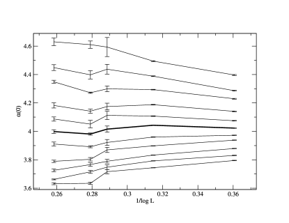
Figure 1: Estimation of the localization edge for $\Delta=1.5$. Each line is at a different frequency, from $\omega^{2}=9.3$ at the bottom to $9.5$ at the top in steps of $0.02$. The critical frequency is that at which this line has zero gradient. Notice the bold line shown, with approximately zero gradient, corresponds to $\omega^{2}=9.4$ and is at $\alpha(0)=4.0$

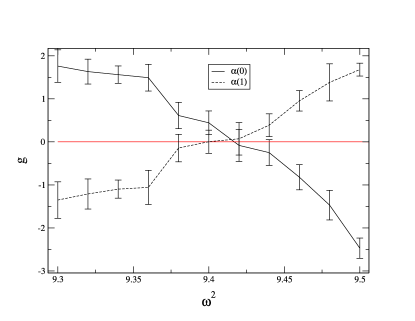
Figure 2: Plot of $g=\textrm{d}\alpha(q)/\textrm{d}(log{L})^{-1}$ for $q=0$ and $1$. The squared critical frequency $\omega_{*}^{2}$ is given by the zero-crossing point of the graph. In this case, $\omega_{*}^{2}$ is between 9.4 and 9.44.

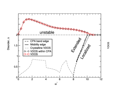
Figure 3: Phase diagram showing the boundary between extended and localized states. The VDOS for the crystal and the lattice with $\Delta=2.0$ have also been plotted to show the location of the mobility edge, $\omega_{*}^{2}$, within the band tail. The band edge calculated with CPA is also shown for reference.

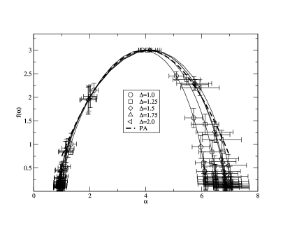
Figure 4: Critical spectra for the force-constant disordered models. The parabolic approximation (PA) to Wegner’s result Wegner_89 is shown for comparison.

Initially, the analysis was undertaken throughout the acoustic band. We did not expect to find localization at the lower (zero-frequency) band edge Taraskin_01:PRL , and indeed it was found that there was only one LD phase transition, located in the far high-energy band tail. The band edge calculated within the coherent potential approximation (CPA) was found to be quite close to the true localization threshold, as can be seen in Fig.3, and therefore it can be used as a rough estimate for the frequency of the actual LD transition .

Having found the mobility edge for several values of force-constant disorder $\Delta$, we can plot these to produce a ’phase diagram’ of the eigenmodes. This is shown alongside the VDOS and the CPA band edge in Fig.3. As the localization edge is in the band tail and we are limited to finite-size systems, few states are localized. With increasing $\Delta$, the mobility edge decreases in frequency with respect to the CPA band edge. However, since the band is broadening, the result is that the critical frequency actually increases with disorder, and thus there is no vibrational analogue to the electronic MIT. Similar behaviour of the mobility edge with disorder can be seen in the phase diagram of the Anderson model with off-diagonal disorder Cain_99 .

For each degree of disorder, we obtain a new critical spectrum which is constant for each size. These critical spectra have been plotted in Fig.4, showing that for positive values of q, i.e. the left hand side of the graph, all the spectra fit onto a master curve. The parabolic approximation (PA) to Wegner’s analytic result Wegner_89 is one which goes through the critical points $f(\alpha=4)=3$ and $f(\alpha=2)=2$, where the latter corresponds to the information dimension of the eigenmode. This PA has also been plotted on the graph for comparison. Note that the Wegner result is for the electronic Anderson model, yet it still fits well with the vibrational data, indicating a universality across the two different systems. The large error bars at high $\alpha$ are in the region where $q$ is negative, where $f$ and $\alpha$ are strongly dependent on the smallest values of the measure and where the errors in the eigenmodes themselves are largest.

To conclude, we have investigated the localization phenomenon for vibrational excitations in disordered structures, using an f.c.c. lattice model with force-constant disorder for analysis. Using MFA, we have confirmed the existence of only one LD transition in the acoustic band, and found the energy at which it occurs for different degrees of disorder. The eigenmodes at the threshold have been shown to be multifractal states exhibiting a quantitatively similar distribution function to that of the critical states in the electron Anderson model.

We are grateful to R.Römer for supplying us with MFA code romercode , and to M.Schreiber for instructive communications.

References

- (1) P. W. Anderson, Phys. Rev. 109, 1492 (1958).
- (2) B. Kramer and A. MacKinnon, Rep. Prog. Phys. 56, 1469 (1993).
- (3) M. Schreiber, in Computational Physics, edited by M. S. K.H.Hoffmann (Springer, 1996), pp. 147–165.
- (4) M. Janssen, Phys. Rep. 295, 1 (1998).
- (5) A. MacKinnon and B. Kramer, Phys. Rev. Lett. 5, 1546 (1981).
- (6) P. Cain, R. Romer, and M. Schreiber, Ann. Phys. (Leipzig) 8, 507 (1999).
- (7) J. L. Pichard and G. Sarma, J. Phys. C 14, L127 (1981).
- (8) P. Carpena and P. Bernaola-Galvan, Phys. Rev. B 60, 201 (1999).
- (9) J. Edwards and D. Thouless, J. Phys. C 5, 807 (1972).
- (10) A. D. Mirlin, Phys. Rep. 326, 259 (2000).
- (11) M. Janssen, Int. J. Mod. Phys. B 8, 943 (1994).
- (12) M. Schreiber and H. Grussbach, Phys. Rev. Lett. 67, 607 (1991).
- (13) H. Grussbach and M. Schreiber, Phys. Rev. B 51, 663 (1995).
- (14) F. Milde, R. A. Römer, and M. Schreiber, Phys. Rev. B 55, 9463 (1997).
- (15) F. Wegner, Nucl. Phys. B 316, 663 (1989).
- (16) R. J. Elliott, J. A. Krumhansl, and P. L. Leath, Rev. Mod. Phys. 46, 465 (1974).
- (17) H. Peitgen, H. Jurgens, and D. Saupe, Chaos and Fractals - New Frontiers of Science (Springer-Verlag, 1992).
- (18) S. N. Taraskin, Y. L. Loh, G. Natarajan, and S. R. Elliott, Phys. Rev. Lett. 86, 1255 (2001).
- (19) We have used the package ARPACK (http://www.caam.rice.edu/software/ARPACK) with sparse matrix inversion routines from the HSL (http://hsl.rl.ac.uk/)
- (20) Both the German MFA and our own MFA code gave practically identical results.