Coulomb couplings in positively charged fullerene

Abstract

We compute, based on density-functional electronic-structure calculations, the Coulomb couplings in the $h_{u}$ highest occupied orbital of molecular C₆₀. We obtain a multiplet-averaged Hubbard $U\simeq 3$ eV, and four Hund-rule-like intra-molecular multiplet-splitting terms, each of the order of few hundreds of meVs. According to these couplings, all C${}_{60}^{n+}$ ions should possess a high-spin ground state if kept in their rigid, undistorted form. Even after molecular distortions are allowed, however, the Coulomb terms still appear to be somewhat stronger than the previously calculated Jahn-Teller couplings, the latter favoring low-spin states. Thus for example in C${}_{60}^{2+}$, unlike C${}_{60}^{2-}$, the balance between Hund rule and Jahn Teller yields, even if marginally, a high-spin ground state. That seems surprising in view of reports of superconductivity in field-doped C${}_{60}^{n+}$ systems.

1 Introduction

Strong electron correlations in multi-band, orbitally degenerate systems represent an important current theoretical challenge. A lively experimental playground for that is provided by electron-doped fullerene systems, which exhibit a variety of behavior, including unconventional metals like cubic CsC₆₀ (Brouet et al. 1999), superconductors of the A₃C₆₀ family (A= K,Rb,Cs) (Ramirez 1994, Gunnarsson 1997), and insulators, presumably of the Mott-Jahn-Teller type (Fabrizio et al. 1997, Capone et al. 2000), such as Na₂C₆₀ (Brouet et al. 2001), A₄C₆₀ (Benning et al. 1993), and the class of ammoniated compounds (NH₃)K_3-xRb_xC₆₀.

The recently developed C₆₀ field effect transistor (FET) devices (Schön et al. 2000a,b) claimed metallic and superconducting states for both electron and hole doping in the interface C₆₀ layer, the hole-doped system showing generally higher $T_{c}$ than the electron-doped system. That could be related to a larger electron-phonon (e-ph) coupling of the HOMO-derived $h_{u}$ band than for the LUMO-derived $t_{1u}$ band (Manini et al. 2001).

However, in an orbitally degenerate system like the one at hand, the electron-phonon coupling competes against intra-molecular exchange of Coulomb origin, responsible for Hund rules. In fact, Hund rules generally favor high spin for a degenerate molecular state, whereas coupling to intra-molecular vibrations leads to a Jahn-Teller (JT) splitting of the degeneracy which favors low spin. Furthermore, since doped fullerenes are narrow-band molecular conductors, knowledge of the local Coulomb repulsion, usually parametrized by the so-called Hubbard $U$, is important in order to establish whether C${}_{60}^{n+}$ conductors are weakly or strongly correlated electron systems. In the former case, a conventional Eliashberg-type approach should be adequate to explain superconductivity. In the latter, a new theoretical framework is most likely needed (Fabrizio et al. 1997, Capone et al. 2000, Capone et al. 2002).

All these considerations stress the importance of a realistic estimate of the Coulomb interaction terms (Hubbard $U$ and the Hund multiplet terms) for C${}_{60}^{n+}$. In the past, electronic-structure-based calculations of these parameters have been made for the negative ions C${}_{60}^{n-}$, where the electrons are added to the $t_{1u}$ LUMO. In that case the structure of the Coulomb Hamiltonian is formally the same as that for an atomic $p$ level in spherical symmetry, and as such entirely determined by two parameters only: the configuration-averaged $U$ and Hund-rule intra-molecular exchange $J$ (Martin and Ritchie 1993, Han and Gunnarsson 2000). For positive ions C${}_{60}^{n+}$, where $n$ holes are added to the $h_{u}$ HOMO the only estimate available for the Coulomb parameters is a recent empirical one (Nikolaev and Michel 2002). The task of an electronic structure-based first principles calculation of these parameters will be the main purpose of the present paper.

In a fivefold-degenerate $h_{u}$ orbital, as we shall detail below, icosahedral symmetry determines these Coulomb couplings in terms of five independent parameters: a configuration-averaged $U$, plus four intra-molecular exchange terms. All the low-energy electronic degrees of freedom of a solid-state system of positively (or negatively) charged C₆₀ molecules can be well described by a model Hamiltonian including the five $h_{u}$ hole bands (or three $t_{1u}$ electron bands) only, all other orbitals acting, as usual, as a mere source of renormalization of the ‘bare’ parameter values (Han and Gunnarsson 2000).

In order to calculate the five independent intra-molecular electron-electron (e-e) Coulomb parameters, we use standard density-functional electronic-structure calculations in the local (spin) density approximation [L(S)DA], imposing as a constraint different values of the electronic occupation number in the individual Kohn-Sham (KS) orbitals. We carry out several frozen-geometry single-molecule constrained-LDA calculations of the total energy for a variety of charge and spin states of undistorted icosahedral C${}_{60}^{n+}$. By comparing these energies with the corresponding analytic expressions for the model Hamiltonian, which is expressed in terms of the five unknown Coulomb parameters, we finally determine all of them.

As the calculations are carried out for an isolated molecule, the computed Coulomb parameters are effective values, which contain the screening due to the polarizability of the filled molecular orbitals in the molecule, but contain neither the screening due to the other molecules nor that of the conduction electrons in the solid. As a reliability check, we also recompute with the same method the e-e $U$ and $J$ parameters for the LUMO band. The results are found in good agreement with previous estimates (Martin and Ritchie 1993, Han and Gunnarsson 2000, Antropov et al. 1992), which further confirms the viability of our method.

With the Coulomb parameters in hand we can then compute the multiplet spectrum for any given molecular occupancy, $n$ =1,…5. This spectrum strictly applies only to ideal rigid C₆₀ ions, and is not of direct experimental relevance, because it leaves JT distortion effects out. The latter can be crudely estimated using the hole-vibration couplings previously calculated in C₆₀ (Manini et al. 2001) either at second-order in perturbation theory, corresponding to a full neglect of retardation effects, the so-called ‘anti-adiabatic’ approximation, or in the opposite ‘adiabatic’ limit. In the anti-adiabatic approximation, the effective e-e interaction is simply the superposition of the Coulomb repulsion and the phonon-mediated attraction. The total net result as far as $U$ is concerned is still repulsive, the large Coulomb term only marginally corrected by molecular distortions. All the other intra-molecular exchange terms are instead heavily reduced. However, while in the case of C${}_{60}^{n-}$ that leads to an effective sign reversal from Hund to ‘anti-Hund’, (and from repulsive to attractive for an electron pair in the singlet channel) the balance is much less definite for C${}_{60}^{n+}$, where the overall sign remains positive for $n$=2 and is uncertain for higher $n$ values. The efficiency of the JT effect in reversing Hund-rules couplings for C${}_{60}^{n+}$ is even weaker when the adiabatic approximation is considered instead of the anti-adiabatic one. In the adiabatic approximation, where ionic motion is classical, the molecular ground state of C${}_{60}^{n+}$ turns out to be always high spin for all $n$ values, in contrast to C${}_{60}^{n-}$ where it is always low spin.

This paper is organized as follows: Sec. 2 introduces the model, determining the minimal number of independent parameters consistent with icosahedral symmetry. The constrained-LDA calculation and its results are described in Sec. 3. The multiplet spectra resulting from the computed couplings are shown in Sec. 4. The results are discussed in Sec. 5, and some lengthy formulae are collected in an Appendix.

2 The model Hamiltonian

Our final target is to address the low-energy properties of (a lattice of) charged C₆₀ molecules. To this end we construct a model Hamiltonian to describe the physics of either the $h_{u}$ HOMO (holes) or $t_{1u}$ LUMO (electrons) bands. The role of the other orbitals is to act as a renormalization of the effective parameters for the band at the Fermi energy. In this paper we concentrate on the determination of single-molecule properties, and defer to a future work the calculation of the bands in the solid. The model Hamiltonian for a single molecule reads

$$\hat{H}=\hat{H}_{0}+\hat{H}_{\rm vib}+\hat{H}_{\rm e-vib}+\hat{H}_{\rm e-e}$$ (1)

where

$$\hat{H}_{0} = \epsilon\,\sum_{\sigma m}\hat{c}^{\dagger}_{\sigma m}\hat{c}_{\sigma m}$$ (2)

$$\hat{H}_{vib} = \sum_{i\Lambda\mu}\frac{\hbar\omega_{i\Lambda}}{2}(\hat{P}_{i\Lambda\mu}^{2}+\hat{Q}_{i\Lambda\mu}^{2})$$ (3)

$$\hat{H}_{\rm e-vib} = \sum_{r\,i\Lambda}\frac{g^{r}_{i\Lambda}\hbar\omega_{i\Lambda}}{2}\sum_{\sigma mm^{\prime}\mu}C^{r\Lambda\mu}_{mm^{\prime}}\,\hat{Q}_{i\Lambda\mu}\,\hat{c}^{\dagger}_{\sigma m}\hat{c}_{\sigma m^{\prime}}$$ (4)

$$\hat{H}_{\rm e-e} = \frac{1}{2}\sum_{\sigma,\sigma^{\prime}}\sum_{{mm^{\prime}}\atop{nn^{\prime}}}w_{\sigma,\sigma^{\prime}}(m,m^{\prime};n,n^{\prime})\,\hat{c}^{\dagger}_{\sigma m}\hat{c}^{\dagger}_{\sigma^{\prime}m^{\prime}}\,\hat{c}_{\sigma^{\prime}n^{\prime}}\hat{c}_{\sigma n}.$$ (5)

are respectively the single-particle Hamiltonian, the vibron contribution (in the harmonic approximation), the electron-vibron coupling (in the linear JT approximation) (Manini et al. 2001, Manini and De Los Rios 2000), and the mutual Coulomb repulsion between the electrons. The $\hat{c}^{\dagger}_{\sigma,m}$ denote the creation operators of either a hole in the HOMO or an electron in the LUMO, described by the single-particle wave function $\varphi_{m\sigma}({\bf r})$. $\sigma$ indicates the spin projection, $m$ and $n$ label the component within the degenerate electronic HOMO/LUMO multiplet, and $i$ counts the phonon modes of symmetry $\Lambda$ (2 $A_{g}$, 6 $G_{g}$ and 8 $H_{h}$ modes). $C^{r\Lambda\mu}_{mn}$ are Clebsch-Gordan coefficients of the icosahedron group, for coupling two $h_{u}$ (holes) or $t_{1u}$ (electrons) states to phonons of symmetry $\Lambda$. $r$ is a multiplicity label, relevant for $H_{g}$ modes only (Manini et al. 2001, Butler 1981). $\hat{Q}_{i\Lambda\mu}$ and $\hat{P}_{i\Lambda\mu}$ are the molecular phonon coordinates and conjugate momenta. Spin-orbit is exceedingly small (Tosatti et al. 1996), and it is therefore neglected.

The Coulomb matrix elements are defined by:

$$w_{\sigma,\sigma^{\prime}}(m,m^{\prime};n,n^{\prime})=\int\!\!{\rm d}^{3}r\!\int\!\!{\rm d}^{3}r^{\prime}\,\varphi^{*}_{m\sigma}({\bf r})\,\varphi^{*}_{m^{\prime}\sigma^{\prime}}({\bf r}^{\prime})\,u_{\sigma,\sigma^{\prime}}({\bf r},{\bf r}^{\prime})\,\varphi_{n\sigma}({\bf r})\,\varphi_{n^{\prime}\sigma^{\prime}}({\bf r}^{\prime})$$ (6)

where $u_{\sigma,\sigma^{\prime}}({\bf r},{\bf r}^{\prime})$ is an effective Coulomb repulsion, screened by the other electrons of the molecule.

One way to estimate these matrix elements is to evaluate the Coulomb integrals (6) directly for the simple kernel $u_{\sigma,\sigma^{\prime}}({\bf r},{\bf r}^{\prime})=q_{e}^{2}/(4\pi\epsilon_{0}|{\bf r}-{\bf r}^{\prime}|)$ and given molecular orbitals (Nikolaev and Michel 2002). This approach neglects completely the screening due to the other electrons on the same molecule. Here we choose a rather different approach: namely, we parametrize the interaction Hamiltonian (5) in the most general way allowed by the molecular symmetry, and then determine the parameters by fitting to ab initio electronic structure calculations. As these calculations allow for the full polarization response of the total charge density (except for core levels, whose polarizability is negligible by comparison) the screening effect of all molecular valence electrons is accounted for in the final parameters.

The symmetry of the Coulomb interaction plus the molecular symmetry of the problem allow us to express all of the Coulomb integrals in (6) as functions of a small set of physical parameters. In the following, we obtain the minimal set of Coulomb parameters that determine the interaction Hamiltonian (5), as required by the symmetry of the molecule and the symmetry label of the orbitals under consideration.

As the Hamiltonian is time-reversal invariant, the orbitals can be chosen real with no loss of generality. Furthermore we take the orbitals, as well as the interaction, to be spin-independent (thus neglecting spin-dependent screening effects which might be possible in magnetic states), so that:

$$w_{\sigma,\sigma^{\prime}}(m,m^{\prime};n,n^{\prime})=w(m,m^{\prime};n,n^{\prime})=\int\!\!{\rm d}^{3}r\!\int\!\!{\rm d}^{3}r^{\prime}\,\varphi_{m}({\bf r})\,\varphi_{m^{\prime}}({\bf r}^{\prime})\,u({\bf r},{\bf r}^{\prime})\,\varphi_{n}({\bf r})\,\varphi_{n^{\prime}}({\bf r}^{\prime})\ .$$ (7)

With the above assumptions one finds immediately:

$$w(m,m^{\prime};n,n^{\prime})=w(n,m^{\prime};m,n^{\prime})=w(m,n^{\prime};n,m^{\prime})=w(n,n^{\prime};m,m^{\prime})\ .$$ (8)

The effective screened interaction shows the full molecular symmetry, i.e.

$$u({\bf R}\,{\bf r},{\bf R}\,{\bf r}^{\prime})=u({\bf r},{\bf r}^{\prime})$$ (9)

for all the symmetry operations ${\bf R}$ of the icosahedral group $I_{h}$. In order to make use of this symmetry, we decompose the product wave functions into irreducible representations of the icosahedral group:

$$\varphi_{m}({\bf r})\,\varphi_{n}({\bf r})=\sum_{r,\Lambda,\mu}C^{r\Lambda\mu}_{mn}\Phi^{r\Lambda}_{\mu}({\bf r})\ ,$$ (10)

using again the Clebsch-Gordan coefficients $C^{r\Lambda\mu}_{mn}$ to couple two $h_{u}$ (holes) or $t_{1u}$ (electrons) tensors to an irreducible tensor of symmetry $\Lambda$. The label $\Lambda$ runs in principle on all the irreducible representations ($A_{g}$, $T_{1g}$, $T_{2g}$, $G_{g}$, $H_{g}$, $A_{u}$, $T_{1u}$, $T_{2u}$, $G_{u}$, $H_{u}$) of the icosahedral group $I_{h}$. The multiplicity label $r$ distinguishes between multiple occurrences of the same representation in the coupling (10): it is the standard extra label for groups, such as $I_{h}$, which are not simply reducible (Butler 1981). Due to the symmetry relation (8), only the symmetric couplings occur. In particular, for holes in the HOMO, from the decomposition of $h_{u}\otimes h_{u}$ the only nonzero contributions come from $\Lambda=A_{g}$, $G_{g}$, $H_{g}^{(r=1)}$, and $H_{g}^{(r=2)}$. For electrons in the $t_{1u}$ LUMO, we have $\Lambda=A_{g}$ and $H_{g}$ only. In terms of this symmetry recoupling, we rewrite the Coulomb matrix elements as:

$$w(m,m^{\prime};n,n^{\prime})=\!\!\!\sum_{{r,\Lambda,\mu}\atop{r^{\prime},\Lambda^{\prime},\mu^{\prime}}}\!\!C^{r\Lambda\mu}_{mn}\,C^{r^{\prime}\Lambda^{\prime}\mu^{\prime}}_{m^{\prime}n^{\prime}}\!\int\!\!{\rm d}^{3}r\int\!\!{\rm d}^{3}r^{\prime}\,\Phi^{r\Lambda}_{\mu}({\bf r})\,u({\bf r},{\bf r}^{\prime})\,\Phi^{r^{\prime}\Lambda^{\prime}}_{\mu^{\prime}}({\bf r}^{\prime})\ .$$ (11)

This equation shows the decomposition of the $w(m,m^{\prime};n,n^{\prime})$ interaction matrix into the sum of products of geometric factors (Clebsch-Gordan coefficients), times a relatively restricted number of coupled matrix elements. We can now exploit the symmetry of the Coulomb interaction (9) to further simplify the remaining integrals. To this end, we apply a generic group operation ${\bf R}$ to the integration variables. The explicit transformation properties of the coupled wave functions $\Phi^{r\Lambda}_{\mu}({\bf r})$ allows to introduce the group representation matrices $\Gamma^{\Lambda}_{\mu_{1}\mu}({\bf R})$, while the effective interaction remains invariant. Next, we apply the grand orthogonality theorem of representation theory, to rewrite the interaction as follows:

$$\int\!\!{\rm d}^{3}r\int\!\!{\rm d}^{3}r^{\prime}\Phi^{r\Lambda}_{\mu}({\bf r})\,u({\bf r},{\bf r}^{\prime})\,\Phi^{r^{\prime}\Lambda^{\prime}}_{\mu^{\prime}}({\bf r}^{\prime})$$ (12)

$$= \int\!\!{\rm d}^{3}r\int\!\!{\rm d}^{3}r^{\prime}\Phi^{r\Lambda}_{\mu}({\bf R}^{-1}{\bf r})\,u({\bf R}^{-1}{\bf r},{\bf R}^{-1}{\bf r}^{\prime})\,\Phi^{r^{\prime}\Lambda^{\prime}}_{\mu^{\prime}}({\bf R}^{-1}{\bf r}^{\prime})$$

$$= \sum_{\mu_{1}\mu_{1}^{\prime}}\Gamma^{\Lambda}_{\mu_{1}\mu}({\bf R})\Gamma^{\Lambda^{\prime}}_{\mu_{1}^{\prime}\mu^{\prime}}({\bf R})\int\!\!{\rm d}^{3}r\int\!\!{\rm d}^{3}r^{\prime}\Phi^{r\Lambda}_{\mu_{1}}({\bf r})\,u({\bf r},{\bf r}^{\prime})\,\Phi^{r^{\prime}\Lambda^{\prime}}_{\mu_{1}^{\prime}}({\bf r}^{\prime})$$

$$= \delta_{\Lambda,\Lambda^{\prime}}\delta_{\mu,\mu^{\prime}}\underbrace{\frac{1}{|\Lambda|}\sum_{\mu_{1}}\int\!\!{\rm d}^{3}r\int\!\!{\rm d}^{3}r^{\prime}\Phi^{r\Lambda}_{\mu_{1}}({\bf r})\,u({\bf r},{\bf r}^{\prime})\,\Phi^{r^{\prime}\Lambda}_{\mu_{1}}({\bf r}^{\prime})}_{F^{r,r^{\prime},\Lambda}}.$$

This shows that the integrals in Eq. (11) are diagonal in the representation label (but not in the multiplicity label $r$). This relation determines explicitly the most general expression for the Coulomb matrix elements in a shell of $t_{1u}$ or $h_{u}$ icosahedral label, in terms of a minimal set of independent parameters $F^{r,r^{\prime},\Lambda}$ [defined in Eq. (12)]:

$$w(m,m^{\prime};n,n^{\prime})=\sum_{r,r^{\prime},\Lambda}F^{r,r^{\prime},\Lambda}\left(\sum_{\mu}C^{r\Lambda\mu}_{mn}\,C^{r^{\prime}\Lambda\mu}_{m^{\prime}n^{\prime}}\right)\ .$$ (13)

In this paper we label states within the degenerate representation using the $C_{5}$ quantum number $m$ from the $I_{h}\supset D_{5}\supset C_{5}$ group chain (Butler 1981). Note however that the purely geometric decomposition of the Coulomb integrals (13) holds for any choice of the group chain, and correspondingly of the $I_{h}$ Clebsch-Gordan coefficients.

In the case of electron doping in the $t_{1u}$ orbital, no multiplicity $r$ labels appears, and thus, according to Eq. (13), the Coulomb Hamiltonian is expressed as the sum of two terms, whose strength is governed by the two parameters $F^{A_{g}}$ and $F^{H_{g}}$. These parameters are related to the $k=0$ and $k=2$ Slater-Condon integrals $F^{(k)}$ for $p$ electrons in spherical symmetry (Cowan 1981). For hole doping in the $h_{u}$ HOMO, we need five parameters

$$F_{1}=F^{A_{g}},\ F_{2}=F^{G_{g}},\ F_{3}=F^{1,1,H_{g}},\ F_{4}=F^{2,2,H_{g}},\ F_{5}=F^{1,2,H_{g}}$$ (14)

to determine completely the Coulomb matrix elements . In terms of spherical symmetry for a $d$ atomic state, $F^{(0)}$ again corresponds to the totally symmetric $F^{A_{g}}$ parameter, while the $F^{(2)}$ and $F^{(4)}$ spherical parameters are replaced by the four icosahedral $F_{2\div 5}$.

Rather than the $F^{\Lambda}$ parameters, for $t_{1u}$ electrons it is more common to use the parameters $U=F^{A_{g}}/3-F^{H_{g}}/3$, and $J=F^{H_{g}}/2$. With this definition of $U$ , the multiplet-averaged energy has the simple dependence on the total number of electrons $n$:

$$E^{\rm ave}(n)={\rm Tr}(H|_{n})=\epsilon n+U\frac{n(n-1)}{2}\ ,$$ (15)

where $H|_{n}$ is the Hamiltonian restricted to the $n$-electrons states. The $J$ parameter controls the multiplet exchange splittings, so that the center of mass of the multiplets at fixed $n$ and total spin $S$ is given by

$$E^{\rm ave}(n,S)={\rm Tr}(H|_{n,S})=\epsilon\,n+U\frac{n(n-1)}{2}-\frac{5}{4}J\left[S(S+1)-\frac{9}{10}n+\frac{3}{20}n^{2}\right].$$ (16)

For the $h_{u}$ holes, the center of mass of the multiplets with $n$ holes is located at energy

$$E^{\rm ave}(n)=\epsilon\,n+\left(\frac{F_{1}}{5}-\frac{4\,F_{2}}{45}-\frac{F_{3}}{9}-\frac{F_{4}}{9}\right)\frac{n(n-1)}{2}.$$ (17)

This leads to the definition of an average Coulomb repulsion

$$U=\left(\frac{F_{1}}{5}-\frac{4\,F_{2}}{45}-\frac{F_{3}}{9}-\frac{F_{4}}{9}\right).$$ (18)

We can define a spin-splitting parameter $J$ also for the holes, by considering the center of mass of the multiplets at fixed spin $S$, $E^{\rm ave}(n,S)$. We find that the Coulomb Hamiltonian (5) is consistent with

$$E^{\rm ave}(n,S)=\epsilon\,n+U\frac{n(n-1)}{2}-J\left[S(S+1)-\frac{5}{6}n+\frac{1}{12}n^{2}\right],$$ (19)

with

$$J=\frac{1}{6}F_{2}+\frac{5}{24}\left(F_{3}+F_{4}\right).$$ (20)

In what follows we take as a convenient set of independent Coulomb parameters: $U$, $F_{2}$, $F_{3}$, $F_{4}$, and $F_{5}$.

Finally, with the decomposition (13) in hand, it is convenient to re-organize the interaction Hamiltonian (5) in terms of number-conserving symmetry-adapted fermion operators:

$$\hat{H}_{\rm e-e}=\frac{1}{2}\sum_{rr^{\prime}\Lambda}F^{r,r^{\prime},\Lambda}\left(\sum_{\mu}\hat{w}^{r\Lambda\mu}\,\hat{w}^{r^{\prime}\Lambda\mu}\right)-A\hat{n}$$ (21)

where we defined the operators:

$$\hat{w}^{r\Lambda\mu}:=\sum_{\sigma}\sum_{mn}C^{r\Lambda\mu}_{mn}\,\hat{c}^{\dagger}_{\sigma m}\hat{c}_{\sigma n}$$ (22)

and the constant $A$, which is $\left(\frac{1}{2}U+\frac{8}{3}J\right)$ for holes and $\left(\frac{1}{2}U+2J\right)$ for electrons.

3 Determination of the Coulomb parameters

After the explicit derivation of the form of a general icosahedral e-e interaction $\hat{H}_{\rm e-e}$, we come now to the numerical calculation of the parameters fixing the interaction for C₆₀ ions. We compute these parameters by comparing the (analytical) expressions for the energies in the model Hamiltonian (1) with numerical results, obtained by first-principles density-functional theory (DFT) LDA calculations of the electronic structure of the C₆₀ molecule.

As the Coulomb Hamiltonian governs the spectrum of multiplet excited states of the ionized configurations, in principle it would be straightforward to obtain the Coulomb parameters by fitting the excitation energies of (1) to multiplet energies obtained with some ab-initio method, or to experimental multiplet spectra, if they were available and if the e-ph contribution could be separated out. However, to our knowledge no such experimental data are till now available. We thus choose to extract the Coulomb parameters from DFT calculations. Yet this is not straightforward, since in standard DFT the excitation energies of the KS system do not have a rigorous physical meaning; the KS states are only auxiliary quantities (Perdew 1985). Although excitation energies are accessible in DFT within the framework of time-dependent DFT (Petersilka et al. 1996), here we follow an alternative approach which is similar in spirit to the constrained-LDA (Dederichs et al. 1984, Gunnarsson et al. 1989) method to extract effective local Coulomb parameters. In a nutshell, constrained-LDA yields the ground-state energy of the system subject to some external constraint, such as a fixed magnetization or a fixed orbital occupancy. In practice, it is convenient to impose constraints such as to select states which are single Slater determinants, since they are described fairly accurately by standard LDA methods. By comparing their total energies with the expectation values of the model Hamiltonian with respect to the same states, it is possible to determine the interaction parameters, in the spirit of the $\Delta$SCF (self-consistent field) scheme (Jones and Gunnarsson 1989).

In order to describe the method, it is convenient to consider a simple example. Let us focus on the states $|n_{\uparrow},n_{\downarrow};0,0;0,0\rangle$ in the LUMO subspace where $n_{\uparrow}$ spin up and $n_{\downarrow}$ spin down electrons fill orbital $\varphi_{1}$, the other two orbitals being empty, and define $E^{\rm tot}(n_{\uparrow},n_{\downarrow})$ the corresponding total energies. One could determine the ‘Hubbard $U_{1}$’ relating to this orbital as

$$U_{1}=E^{\rm tot}(1,1)+E^{\rm tot}(0,0)-E^{\rm tot}(1,0)-E^{\rm tot}(0,1)=E^{\rm tot}(1,1)+E^{\rm tot}(0,0)-2E^{\rm tot}(1,0)\ .$$ (23)

A slight complication to this simple approach is brought in our problem by the orbital degeneracy. Suppose we indeed compute by LDA the energy of $|1,1;0,0;0,0\rangle$. This orbital, where we place the two electrons, is initially degenerate to the other two LUMO components. However, in LDA, a Kohn-Sham (KS) filled orbital shifts immediately up in energy with respect to empty ones. Consequently, if we insist to fill one of the three, originally degenerate, KS orbitals, at the next iteration the electrons go naturally to occupy either of the two initially empty orbitals, with a large jump in charge density from one iteration to the next. This effect is due to the imperfect cancellation of the self interaction within LDA , which is also related to the well-known LDA gap problem.

A possible remedy is to artificially introduce small gaps (of the order of 10 meV) in the otherwise degenerate HOMO and LUMO, by adding a tiny distortion of the icosahedral C₆₀ molecule along one of the JT active modes. Since the distortion is very small (each atom moving by less than 0.5 pm from its equilibrium position), the model remains essentially representative of fully symmetric fullerene. However, in order to effectively control the charge (either electrons in the LUMO or holes in the HOMO) in the different orbitals, the splittings must overcome the self-repulsion. This fact suggests occupying an orbital by a small fraction of an electron so that the self repulsion is sufficiently small to leave this orbital in the same energy position dictated by the distortion field.

To recover the actual value of the energy at integer charge, as required for the determination of $U$ according to Eq. (23), we make use of a known artifact of the LSDA: the ground-state energy of a system as a functional of the fractional occupation of a KS orbital interpolates smoothly the energies of integer multiples of the elementary charge. To the extent that the modifications of orbital $\phi_{1}$ due to changes of its filling $n_{1}$ may be neglected, the total energy is a parabolic function of charge. In particular, in our specific example,

$$E^{\rm tot}\left(\frac{n_{1}}{2},\frac{n_{1}}{2}\right) = E^{\rm tot}_{0}+b\,n_{1}+\frac{c}{2}\,n_{1}^{2}\ ,$$

$$E^{\rm tot}\left(n_{1},0\right) = E^{\rm tot}_{0}+b^{\prime}\,n_{1}+\frac{c^{\prime}}{2}\,n_{1}^{2}\ ,$$ (24)

where, according to Janak’s theorem (Janak 1978), the linear coefficients $b=b^{\prime}$ equal the KS single-particle energy $\epsilon_{1}$ at $n_{1}\to 0$. The quadratic coefficients $c$ and $c^{\prime}$ are not generally the same, since they are extracted from unpolarized and spin-polarized configurations, respectively. We have verified, in those configurations where the self interaction causes no convergence problem, that the extrapolation from calculations at $n_{1}\leq 0.2$ is in very good quantitative agreement with direct total-energy calculations at integer $n_{1}$’s. Through Eqs. (24) and (23) we have:

$$U_{1}=\left(E^{\rm tot}_{0}+b\cdot 2+\frac{c}{2}\cdot 2^{2}\right)+E^{\rm tot}_{0}-2\left(E^{\rm tot}_{0}+b^{\prime}+\frac{c^{\prime}}{2}1^{2}\right)=(2c-c^{\prime})\ .$$ (25)

We have therefore expressed the Hubbard $U_{1}$ as a linear combination of the quadratic coefficients $c$ and $c^{\prime}$ of the extrapolation parabolas. Note that the $c$’s for both configurations involved are needed for the determination of $U_{1}$: it would be incorrect to identify $U_{1}$ to, for example, the curvature $c$ of the total LDA energy as a function of charge.

The complete determination of the two and respectively of the five Coulomb parameters for $t_{1u}$ electrons and for $h_{u}$ holes follows the same track as the simple determination of $U_{1}$ outlined above. First, we select two sets of electronic configurations, one for electron and the other for hole doping, containing three (see Table 1) and eight (see Table 2) elements, respectively. For each configuration $|i\rangle$, we compute the total energy as a function of the (fractional) charge, for five values $0\leq n_{i}\leq 0.2$. The calculations for a given set are carried out with a fixed JT distortion within DFT-LSDA. As in previous calculations (Manini et al. 2001) we use ultrasoft pseudopotentials (Vanderbilt 1990) for C (Favot and Dal Corso 1999). The plane-waves basis set is cut off at 27 Ry (charge density cutoff = 162 Ry). The C₆₀ molecule is repeated periodically in a large simple-cubic supercell lattice of side $a$. To insure total charge neutrality, thus correcting for the $G=0$ divergence of the total energy, a compensating uniform background charge is added. The total energy is corrected for the leading power-law Coulomb interactions among supercells, by removing the Madelung $a^{-1}$ term and the $a^{-3}$ correction, with the method devised by Makov and Payne (1995). We extract the finite-$a$ corrections by running several calculations with $a$ ranging between 1.32 and 1.85 nm, as illustrated in Fig. 1 in a typical example. [It might have been marginally cheaper to use the modified Coulomb potential method (Jarvis et al. 1997) instead of the size scaling. That method however required a larger lattice parameter $a$, and thus more memory space]. Parabolas of the form (24) are fitted to the calculated $a\to\infty$ energies. The resulting quadratic coefficients $c_{i}$ for electrons and holes are reported in Tables 1 and 2 respectively.

In the light of Janak’s theorem (Janak 1978), stating that the single-particle KS levels $\epsilon_{i}(n_{i})=\partial E^{\rm tot}(n_{i})/\partial n_{i}$, the $c_{i}$ coefficients, besides representing second derivatives of the total energy w.r.t. charge, can alternatively be seen as first derivatives of the single-particle levels w.r.t. charge, as follows:

$$\epsilon_{i}(n_{i})=\epsilon_{i}(0)+c_{i}\,n_{i}+O(n_{i}^{2})\ .$$ (26)

From the $a$-scaling of the total energy (Makov and Payne 1995), we derive the $a$-scaling of the single-particle KS levels $\epsilon_{i}$, which allows us to compute these quantities for the isolated molecular ion ($a\to\infty$). Equation (26) (neglecting $O(n_{i}^{2})$ corrections) provides a second method to derive the $c_{i}$ coefficients, which are the basic ingredients in the calculation of the Coulomb parameters. As apparent in Tables 1 and 2, the coefficients $c_{i}$ obtained from the total energy and from the single-particle levels are essentially in accord. However, the values from the single-particle levels are numerically more stable since, contrary to the total-energy method, they do not involve small differences of large numbers. In the following we shall use the $c_{i}$’s from single-particle energies for the determination of the Coulomb parameters.

The calculation of the e-e parameters is then realized by equating the various DFT extrapolated energies to the expectation values of (1) with respect to the same electronic configurations. Given the arbitrariness in the reference energy $\epsilon$ for the model Hamiltonian (1), we define for convenience

$$\epsilon=U/2+b_{i}-\mu\ .$$ (27)

where $\mu$ is a free parameter allowing for the possibility of a chemical potential shift with respect to the DFT calculation .

In Table 3 we collect the analytic expression of the energies of the three states considered for $t_{1u}$ electrons. Equating the terms on the third and fourth column of Table 3, we have 3 equations to determine the 3 unknown quantities $U$, $J$ and $\mu$: we obtain the physical parameters simply by inversion of the linear dependency, and by replacing the values of $c_{i}$ in Table 1. We have tabulated the combination $2n_{i}^{-2}\left(\langle i|\hat{H}_{\rm e-e}|i\rangle+Un_{i}/2\right)$ instead of simply $\langle i|\hat{H}_{\rm e-e}|i\rangle$, as each equation involves quantities of the same order of magnitude. By eliminating $\mu$ [in analogy to the one-state example of Eq. (25)], we find for the Coulomb parameters of the negative C₆₀ ions: $U=\frac{6}{5}c_{|\uparrow\downarrow,\uparrow\downarrow,\uparrow\downarrow\rangle}-\frac{1}{5}c_{|0,\uparrow,0\rangle}=3069$ meV and $J=\frac{6}{5}c_{|\uparrow\downarrow,\uparrow\downarrow,\uparrow\downarrow\rangle}-\frac{3}{2}c_{|\uparrow,\uparrow,\uparrow\rangle}+\frac{3}{10}c_{|0,\uparrow,0\rangle}=32$ meV. These values, summarized in Table 4, are in the same range as previous estimates (Martin and Ritchie 1993, Han and Gunnarsson 2000, Antropov et al. 1992).

To produce a reliable estimate of the six unknown quantities (the five e-e parameters plus $\mu$), we consider eight different $h_{u}$ hole states, for whose energies we collect the analytic expressions in Table 5. Therefore we have eight equations in six unknowns: we obtain the best estimate of the physical parameters by adjusting them to minimize the sum of the squared difference between the energies in the third and the fourth column of Table 5. For this overdetermined system of equations, the combination $2n_{i}^{-2}\left(\langle i|\hat{H}_{\rm e-e}|i\rangle+Un_{i}/2\right)$ shows its advantage, that all LSDA calculations weight the same in the fit. This fitting procedure yields the values of the Coulomb parameters for C${}_{60}^{n+}$ collected in Table 6. The standard deviation of the fit (1.4 meV) gives an estimate of the numerical accuracy of the $c_{i}$ parameters. By standard error propagation, we obtain the estimate of the errorbar on the individual e-e parameters reported in Table 6.

We can now comment on our obtained results. We observe first of all that the only large parameter is $U$. It takes essentially the same value in the LUMO and the HOMO: this value of about 3 eV governs the multiplet-averaged hole-hole repulsion, and is also compatible with experimental estimates (Antropov et al. 1992) for isolated molecular ions. In the solid, the screening of the local Coulomb parameters due to the polarizability of all the surrounding C₆₀ molecules could be approximately accounted for in a Clausius-Mossotti scheme (Antropov et al. 1992), and, for C${}_{60}^{n-}$, it may reduce $U$ by roughly a factor 0.5 (Lof et al. 1992). The polarizability screening in the solid is expected to affect $F_{2}\div F_{5}$ much less than $U$. Note however that the actual Hubbard $U$, based on differences of ground-state energies, acquires an $n$-dependent contribution of $F_{2}\div F_{5}$. The appropriate $U^{\rm min}$ are collected in Table 7. The extra intra-molecular contribution is especially large at half filling.

The relative smallness of the intra-molecular parameters compared to $U$ is traced to the very close values of the quadratic coefficients $c_{i}$ (listed in Table 2) for all different configurations $|i\rangle$. In turn, this indicates that, contrary to the strongly localized orbitals of atomic physics, in C₆₀ it does not matter much the relative spin and orbital placement of two electrons in the HOMO or LUMO: they would always feel more or less the same repulsion of roughly 3 eV. The Hund rules are therefore rather weak in C₆₀ ions, because the degenerate orbitals are spread over a carbon shell of 7 Ådiameter, rather than concentrated around a single nucleus. The largest parameter is $F_{3}$ corresponding to the $r=1$ $H_{g}$ symmetry. The $F_{5}$ parameter is the smallest, effectively compatible within error bars with a zero value.

The computed intra-molecular exchange $J$ is almost twice as large in the HOMO than in the LUMO (Tables 4 and 6). Consequently, the splittings (in the order of hundreds of meV) of the $n$-hole Coulomb multiplets are larger for holes than for electrons. We come next to the detailed study of this multiplet spectrum.

4 Multiplet energies

The computed values of the coupling parameters can be used to calculate the multiplet spectrum of $\hat{H}_{\rm e-e}$. We concentrate here on the states of $n$ holes in the fivefold degenerate $h_{u}$ HOMO. In order to diagonalize the Hamiltonian matrix, we wish to take full advantage of symmetry. For each charge $n$, $(I_{h}\supset D_{5})$ orbital label $(\Lambda,\mu$), multiplicity $r$, total spin $S$, and spin projection $M$, we first construct a set of symmetry-adapted states by iteratively coupling the one-hole $h_{u}$ orbitals to all the $(n-1)$-holes states as follows:

$$|n,(\tau^{\prime},\Lambda^{\prime},S^{\prime}),(\Lambda,r),\mu;S,M\rangle = \sum_{\mu^{\prime}\mu^{\prime\prime}}\sum_{M^{\prime}M^{\prime\prime}}C^{r\Lambda\mu}_{\Lambda^{\prime},\mu^{\prime};h_{u},\mu^{\prime\prime}}\,C^{SM}_{S^{\prime},M^{\prime};1/2,M^{\prime\prime}}\,\times$$ (28)

$$|n-1,\tau^{\prime},\Lambda^{\prime},\mu^{\prime};S^{\prime},M^{\prime}\rangle\,\times|1,h_{u},\mu^{\prime\prime};\frac{1}{2},M^{\prime\prime}\rangle$$

where $C^{r\Lambda\mu}_{\Lambda^{\prime},\mu^{\prime};h_{u},\mu^{\prime\prime}}$ and $C^{SM}_{S^{\prime},M^{\prime};1/2,M^{\prime\prime}}$ are the icosahedral and spherical Clebsch-Gordan coefficients taking care of the orbital and spin recoupling respectively, and $\tau^{\prime}$ is the parentage of the $(n-1)$-particle state. The resulting states $|n,(\tau^{\prime},\Lambda^{\prime},S^{\prime}),(\Lambda,r),\mu;S,M\rangle$ (for all possible $\tau^{\prime},\Lambda^{\prime},S^{\prime}$ and $r$) are then orthonormalized to form the set of $n$-hole basis states $|n,\tau,\Lambda,\mu;S,M\rangle$, with $\tau$ counting their parentage.

In this symmetry-adapted basis the Hamiltonian is diagonal with respect to the labels $n,\Lambda,\mu,S$ and $M$ and its eigenvalues are independent of $\mu$ and $M$. This block-diagonal form allows in many cases to compute the analytical expressions for the multiplet energies $E_{\rm mult}$, i.e. the eigenvalues of $\hat{H}_{\rm e-e}-U\hat{n}(\hat{n}-1)/2$, that are collected in Table 8. For $3\leq n\leq 7$, the calculation of the multiplet energies involves the diagonalization of block matrices of size 3 up to 7, where analytical methods are unpractical. For these cases we report the Hamiltonian submatrices for those states in Appendix A. The analytical 3-holes spectrum shows the degeneracy of a $T_{1u}$ and a $T_{2u}$ doublet state, which has been observed and explained in previous work (Oliva 1997, Lo and Judd 1999, Plakhutin and Carbó-Dorca 2000).

The spectrum obtained by substituting the computed parameters of Table 6 into the expressions of Table 8 is collected in Table 9. For all values of $n$, we of course verify Hund-rule behavior, i.e. the high-spin state has the lowest energy. However the first Hund rule leads to comparable splittings to second Hund rule, so that states of different spin are energetically inter-mixed, for $n=4$ and 5. The multiplet structure is similar to what was reported in Ref. (Nikolaev and Michel 2002), with a few differences in the detailed ordering of closely spaced levels. The total spread in the DFT results of Table 9, however, are a factor three smaller than those of that rigid-orbital unscreened calculation (Nikolaev and Michel 2002).

The computed spectrum of Table 9 represents that of ideal rigid icosahedral C₆₀. The coupling of electronic state to the intramolecular vibrations generally leads to JT distortions, involving energy scales that compete with the e-e repulsion and generally favor low-spin states, a sort of anti-Hund rule. The interplay of the Coulomb and e-ph terms originates a complex pattern of vibronic multiplet states that was studied in detail in the simpler case of the negative C₆₀ ions (O’Brien 1996). The HOMO system at hand is much more intricate, due to the interplay of several parameters. Here we shall address this problem at a more approximate level of accuracy.

First we observe that, in the limit where the typical phonon energies $\hbar\omega_{i}$ are much larger than the e-ph energy gains $\sim g_{i}^{2}\hbar\omega_{i}$, the e-ph Hamiltonian treated at second order in $g_{i}$ takes the form of the first term in the right hand side of Eq. (21) (anti-adiabatic or weak-coupling limit). The strengths of the effective e-e interaction parameters are given in terms of the dimensionless couplings $g^{r}_{i\Lambda}$ and frequency $\omega_{i\Lambda}$ by $\tilde{F}^{r,r^{\prime},\Lambda}=-\sum_{i}g^{r}_{i\Lambda}g^{r^{\prime}}_{i\Lambda}\hbar\omega_{i\Lambda}/4$ . Table 6 lists the parameters $\tilde{F}_{i}$ generated by the e-ph, in the notation of Eqs. (14) (18) and (20), compared to the $F_{i}$ Coulomb parameters. At this level of approximation, the e-e and e-ph terms are expressed as sums of formally identical terms, differing only for the value of the parameter multiplying each term. Thus, it is natural to combine the two contributions into a total effective two-body Hamiltonian $\hat{H}_{\rm e-e}^{\rm tot}$ which is formally identical to the definition of Eqs. (5) and (13) but based on total effective e-e parameters given by the algebraic sum of the Coulomb and e-ph parameters. These total effective e-e parameters are listed in the last column of Table 6.

The contributions to $U$ of the $G_{g}$ and $H_{g}$ phonons [Eq. (18)] is larger than the $A_{g}$ term, thus giving a small repulsive phononic multiplet-averaged $\tilde{U}$. However, the huge $F_{1}$ Coulomb ‘monopole’ parameter is barely affected by the $A_{g}$ phonons-originated term. Accordingly, the total multiplet-averaged interaction $U^{\rm tot}$ is left basically unaffected by the phonons contribution, for both the HOMO and the LUMO.

On the contrary, the intra-molecular Hund terms $F_{i}$ are of values comparable to the phononic counterpart, thus leading to a strong cancellation. In particular, for the holes the largest repulsive term $F_{3}$ is reversed by the even larger coupling $\tilde{F}_{3}$ to the $H_{g}^{(r=1)}$ phonon modes. The largest total effective term is $F_{2}$: it remains positive, due to the modest $G_{g}$-phonons–mediated attraction. The corresponding multiplets spectrum, is reported in Table 10, and drawn for $n=2$ and $n=3$ in Fig. 2. For $n=2$ holes the ground state remains a triplet, with a very small gap to the lowest singlet, while low-spin ground states prevail for $n\geq 3$. For electrons, the total effective $J=-25$ meV indicates that low-spin anti-Hund states are to be expected for C${}_{60}^{n-}$, as is indeed observed experimentally in many electron-doped C₆₀ compounds (Kiefl et al. 1992, Zimmer et al. 1995, Lukyanchuk et al. 1995, Prassides et al. 1999).

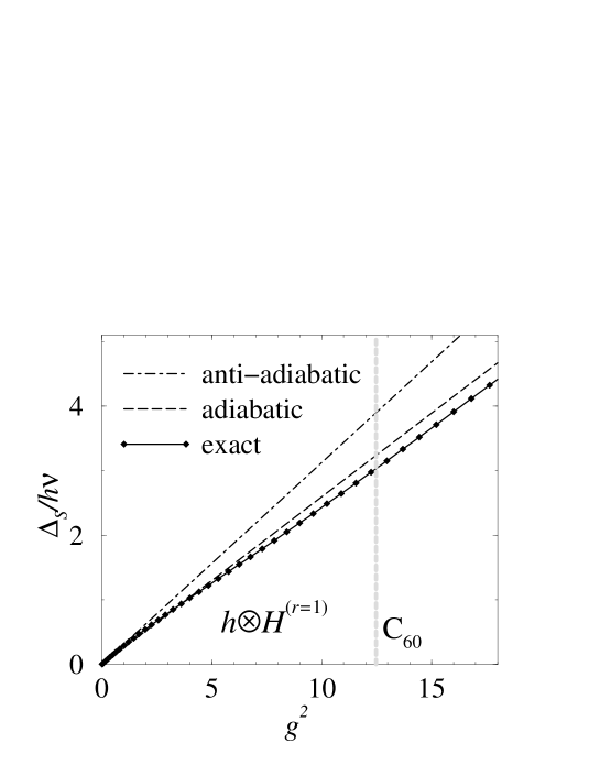
Figure 3: The $n=2$ holes JT spin gap to the lowest triplet state, as a function of the dimensionless linear coupling strength $g^{2}=-4\tilde{F}_{3}/(\hbar\omega)$ of a single $H_{g}$ mode (O’Brien 1972, Manini and Tosatti 1998) (no Coulomb interaction) with pure $r=1$ coupling, similar to the 271 cm^-1 mode of C₆₀, the one with the largest coupling. The same spin gap is plotted for comparison in the anti-adiabatic (dot-dashed – slope 5/16) and adiabatic (dashed – slope 83/320) limits. The vertical bar at $g^{2}=12.5$ locates the total effective $r=1$ coupling of C₆₀ positive ions, according to the DFT estimate of Manini et al. (2001).

The anti-adiabatic approximation, although tending to overestimate the e-ph energies is advantageous in allowing to map the e-ph Hamiltonian onto an effective attractive e-e term: this mapping does not apply any longer when the coupling energies are not taken as much smaller than the harmonic phonon energies. However, the relatively large values of the realistic e-ph coupling in both positive and negative C₆₀ ions make the weak-coupling approximation not truly justified. Indeed the e-ph energetics based on this approximation are grossly overestimated if applied to intermediate/strong couplings. In practice, the JT energy gains and gaps in units of $g_{i}^{2}\hbar\omega_{i}$ become significantly smaller as the coupling changes from weak ($g_{i}\ll 1$) to strong ($g_{i}\gg 1$). In particular, for $t_{1u}$ electrons interacting only with $H_{g}$ modes (no e-e terms), the energy lowering divided by $g_{i}^{2}\hbar\omega_{i}$ drops by 60 % from weak to strong coupling (Manini et al. 1994). For $h_{u}$ holes, for $n=2$ and a single $H_{g}^{(r=1)}$ mode (O’Brien 1972, Manini and Tosatti 1998), we see in Fig. 3 that the spin gap in units of $g^{2}\hbar\omega$ reduces by 17 % only, going from the weak to the strong-coupling limit. However, when all C₆₀ modes are included, this reduction is as large as $\sim$50 % due to contributions of the $H_{g}^{(r=2)}$ and $G_{g}$ modes.

As the actual (anti-Hund) e-ph coupling should have weaker effects than those estimated in the anti-adiabatic approximation, the question of what is the symmetry of the ground state of the C${}_{60}^{n\pm}$ ions remains open. The case of C${}_{60}^{2+}$ marks an exception, since Coulomb couplings prevail already at the anti-adiabatic level (Fig. 2). Thus the prediction of an $S=1$ magnetic ground state for $n$=2 holes in C₆₀ seems fairly robust, at least within LDA accuracy. In order to settle this problem for the other cases, we study the e-ph coupling in the opposite, adiabatic limit, which becomes exact in the limit of strong e-ph coupling, and which proved quantitatively more realistic for C${}_{60}^{n\pm}$ ions (Fig. 3). At the adiabatic level, the phonons are treated classically, with the electrons/holes contributing through (4) to the total adiabatic potential acting on the phonon coordinates $\hat{Q}_{i\Lambda\mu}$ which are treated as classical variables. The additional ingredient we include here, and which was not included in the previous adiabatic calculation (Manini et al. 2001) is the e-e coupling. In the JT-distorted configuration, the icosahedral symmetry is broken, therefore all symmetry states are mixed. Only $n$, $S$ and $S_{z}$ are conserved. For example, the coupling to the distortion of $n=3$ holes, $S=3/2$, $M=3/2$ mixes the 10 states of $T_{1u}$, $T_{2u}$ and $T_{2u}$ symmetry listed in Table 8. Assuming that the Coulomb parameters $F_{i}$ are unchanged upon distortion, for each $n$, $S$ and $M$ we determine the optimal distortion, by full minimization of the lowest adiabatic potential sheet in the space of all the phonons coordinates. In Table 11, we report the resulting lowest-state energy in each spin sector, based on the e-e and e-ph couplings of C${}_{60}^{n\pm}$ ions. As already stated, we find a difference between electrons and holes: the ground state is low spin for C${}_{60}^{2-}$ electrons, while it is always high spin for C${}_{60}^{n+}$. The case of C${}_{60}^{3-}$ has almost degenerate $S=1/2$ and $S=3/2$ states, the former probably prevailing once non-adiabatic corrections are accounted for (Capone et al. 2001). For the positive ions instead, the adiabatic result overturns the anti-adiabatic prediction of low-spin ground state for $n\geq 3$ holes. In these cases, the adiabatic spin gaps are fairly large, and are likely to survive when zero-point quantum corrections to the adiabatic approximations are added. For C${}_{60}^{2+}$ the gap to the lowest singlet state is rather small, but, as noted above, here the ground state is a spin triplet even in the anti-adiabatic approximation: it is likely to remain high spin also within an exact treatment of the phonons.

The outcome of the adiabatic calculation is that positive C₆₀ ions favor high-spin ground states, while in negative ions e-ph coupling prevails and low-spin ground states are likely. However, for C${}_{60}^{n\pm}$ ions the balance of e-e and e-ph is rather delicate, therefore the problem of the spin symmetry of the ground state ions is far from trivial, and remains basically open. Indeed, in some chemical environments high-spin states are observed to prevail in negative fullerene ions (Schilder et al. 1994, Arovas and Auerbach 1995), and this indicates that the lowest multiplets of different spin type are almost degenerate. To get a more conclusive answer on this point for ions of both signs, it would be crucial to carry out a full diagonalization of (1) including all the phonon modes and Coulomb terms on the same ground, on the line of O’Brien (1996): we plan to carry out such calculation in a future work.

5 Discussion and Conclusions

The Coulomb couplings of holes in C₆₀ obtained in this paper are based on rigid icosahedral geometry calculations. However, clearly in each different-charge state, the C${}_{60}^{n\pm}$ molecular ion relaxes to different equilibrium positions, according to the interplay of e-ph coupling ($\hat{H}_{\rm vib}+\hat{H}_{\rm e-vib}$) with intra-molecular Coulomb exchange ($\hat{H}_{\rm e-e}$). In principle one could compute the Coulomb parameters, allowing simultaneously for geometry relaxation. The disadvantage of such a calculation is the difficulty of disentangling the e-ph and e-e contributions. A second difficulty of principle is that the ion, in an electronically degenerate state, distorts to several equivalent static JT minima of less than icosahedral symmetry (Manini and De Los Rios 2000). These local minima are connected by tunneling matrix elements which mix them to suitable dynamical combinations of the different distortions, thus restoring the original icosahedral symmetry: such non-adiabatic situation would be outside the range of applicability of current standard first-principles computational methods, usually based on the Born-Oppenheimer separation of the ionic and electronic motions. Moreover, the lack of exact cancellation of self-interaction in the LDA makes even a practical attempt at a static, adiabatic calculation for JT-distorted ions impossible at this stage. These are the reasons that suggested restricting this first Coulomb calculation to the rigidly undistorted geometry.

A further limitation of the present calculation is the assumption that the Coulomb parameters are independent of the charge of the state. In principle, due to both orbital and geometrical relaxation, the effective Coulomb interaction (6) will depend on the instantaneous charge state of the fullerene ion. However, this effect, a very important one in single-atom calculations, is expected to be fairly small in such a large molecule as C₆₀. Thus our parameters represent an average over $n$.

For C${}_{60}^{n-}$, the value of $J$ was estimated in the 100 meV region by Hartree-Fock calculations (Chang et al. 1991), and by direct integration of the unscreened Coulomb kernel (Nikolaev and Michel 2002). Both these methods overestimate the Coulomb repulsion because of underestimation or complete neglect of screening. The LSDA, where we get $J=32$ meV is on the other hand known to overestimate screening, and thus to underestimate the Coulomb parameters. Some value in between, such as $J\sim 50$ meV, as suggested by Martin and Ritchie (1993) is probably a more realistic estimate of $J$ in C${}_{60}^{n-}$. Coming to the C${}_{60}^{n+}$ case, we can regard the e-e couplings of Table 6 as lower bounds, the actual repulsion being possibly a factor 1.5 or 2 larger. Indeed, the calculation of Nikolaev and Michel (2002) finds splittings about 3 times larger than those of Table 9, and those can reasonably be regarded as upper bounds.

On the other hand, the competing e-ph interaction is also very likely underestimated by LDA, as was demonstrated in the case of C${}_{60}^{-}$ by the comparison of the calculated $g^{2}$ couplings to those extracted from fitting the photoemission spectrum (Gunnarsson et al. 1995), which suggested values roughly twice as large. In that case, the effective e-ph $\tilde{J}$, determined from the photoemission data is $\tilde{J}=-127$ meV compared to the LDA value of $\tilde{J}=-57$ meV. In conclusion, both the Coulomb repulsion and the phonon-mediated attraction calculated within LDA are likely to need a rescaling by a similar factor of order two. Thus the balance between the two opposing interactions remains delicate in both C${}_{60}^{n-}$ [as demonstrated by the presence of both high-spin and low-spin local ground states in different chemical environments (Brouet et al. 2001, Kiefl et al. 1992, Zimmer et al. 1995, Lukyanchuk et al. 1995, Prassides et al. 1999, Schilder et al. 1994, Arovas and Auerbach 1995)] and even more so in C${}_{60}^{n+}$, where however the high-spin states should be more favored. Moreover, especially in the hole doped case, we find multiplet splittings which are comparable to the theoretical bandwidth of solid-state fullerene (about 0.5 eV), indicating that Hund-rule intramolecular interactions are an important ingredient in C₆₀ ions.

Since any treatment of superconductivity caused by the JT coupling must include the competing Hund-rule terms, our results surprisingly indicate that positively-doped C₆₀ could display a weaker tendency toward superconductivity than negatively-doped C₆₀. Magnetic states could occur for any integer hole filling, more commonly than for integer electron fillings. Even if magnetism were to be removed owing to band effects, one should still expect C${}_{60}^{n-}$ to make better superconductors. This conclusion is unexpected in the light of recent data claiming a larger superconducting $T_{c}$ in positively charged than in negatively charged C₆₀ FETs (Schön et al. 2000a,b). The reasons for this disagreement are presently unclear, and will require further theoretical and experimental work.

Appendix A Appendix

We provide here the recipe to construct the matrices $H_{\rm mult}[n,\Lambda,S]$, whose eigenvalues $E_{\rm mult}$ give the $(F_{2}\dots F_{5})$-dependent contribution to the multiplet energies of $n$ holes of global symmetry $\Lambda$ and total spin $S$ in Table 8. Each matrix $H_{\rm mult}[n,\Lambda,S]$ is a linear combination of four numerical matrices $M_{i}[n,\Lambda,S]$ (given below), with as coefficients the Coulomb parameters $F_{2}\dots F_{5}$:

$$H_{\rm mult}[n,\Lambda,S]=\sum_{i=2}^{5}\,F_{i}\,\,M_{i}[n,\Lambda,S]\ .$$ (29)

With specific choice of the parameters, it is possible to study the effect of one particular operator: for example, by taking only $F_{3}\neq 0$, thus diagonalizing the $M_{3}[n,\Lambda,S]$ matrices one may study analytically the multiplet spectrum associated to that operator. To get the spectra of Tables 9 and 10, we plugged the parameters of Table 6 into Eq. (29), and proceeded to diagonalize $H_{\rm mult}[n,\Lambda,S]$ numerically.

The matrices $M_{i}[n,\Lambda,S]$ are as follows:

$$M_{2}[3,H_{u},1/2] = \left(\matrix{\frac{2}{3}&-\frac{2}{{\sqrt{21}}}&{\sqrt{\frac{10}{21}}}&0\cr-\frac{2}{{\sqrt{21}}}&-\frac{2}{21}&-\frac{5\,{\sqrt{\frac{5}{2}}}}{21}&-{\sqrt{\frac{5}{42}}}\cr{\sqrt{\frac{10}{21}}}&-\frac{5\,{\sqrt{\frac{5}{2}}}}{21}&\frac{11}{42}&-\frac{1}{{\sqrt{21}}}\cr 0&-{\sqrt{\frac{5}{42}}}&-\frac{1}{{\sqrt{21}}}&\frac{5}{6}}\right)$$

$$M_{3}[3,H_{u},1/2] = \left(\matrix{\frac{5}{6}&0&0&0\cr 0&\frac{5}{42}&\frac{3\,{\sqrt{\frac{5}{2}}}}{14}&\frac{{\sqrt{\frac{15}{14}}}}{2}\cr 0&\frac{3\,{\sqrt{\frac{5}{2}}}}{14}&-\frac{17}{84}&\frac{{\sqrt{\frac{3}{7}}}}{2}\cr 0&\frac{{\sqrt{\frac{15}{14}}}}{2}&\frac{{\sqrt{\frac{3}{7}}}}{2}&\frac{1}{12}}\right)$$

$$M_{4}[3,H_{u},1/2] = \left(\matrix{\frac{5}{6}&\frac{2}{{\sqrt{21}}}&-{\sqrt{\frac{10}{21}}}&0\cr\frac{2}{{\sqrt{21}}}&\frac{13}{42}&\frac{{\sqrt{\frac{5}{2}}}}{42}&-\frac{{\sqrt{\frac{5}{42}}}}{2}\cr-{\sqrt{\frac{10}{21}}}&\frac{{\sqrt{\frac{5}{2}}}}{42}&\frac{23}{84}&-\frac{1}{2\,{\sqrt{21}}}\cr 0&-\frac{{\sqrt{\frac{5}{42}}}}{2}&-\frac{1}{2\,{\sqrt{21}}}&-\frac{7}{12}}\right)$$

$$M_{5}[3,H_{u},1/2] = \left(\matrix{0&{\sqrt{\frac{15}{7}}}&{\sqrt{\frac{6}{7}}}&0\cr{\sqrt{\frac{15}{7}}}&\frac{2\,{\sqrt{5}}}{7}&-\frac{3}{7\,{\sqrt{2}}}&-\frac{1}{{\sqrt{42}}}\cr{\sqrt{\frac{6}{7}}}&-\frac{3}{7\,{\sqrt{2}}}&-\frac{2\,{\sqrt{5}}}{7}&\frac{{\sqrt{\frac{5}{21}}}}{2}\cr 0&-\frac{1}{{\sqrt{42}}}&\frac{{\sqrt{\frac{5}{21}}}}{2}&0}\right)$$

$$M_{2}[4,A_{g},0] = \left(\matrix{\frac{4}{3}&-\frac{4}{{\sqrt{21}}}&2\,{\sqrt{\frac{10}{21}}}\cr-\frac{4}{{\sqrt{21}}}&-\frac{4}{21}&-\frac{5\,{\sqrt{10}}}{21}\cr 2\,{\sqrt{\frac{10}{21}}}&-\frac{5\,{\sqrt{10}}}{21}&\frac{11}{21}}\right)$$

$$M_{3}[4,A_{g},0] = \left(\matrix{\frac{5}{3}&0&0\cr 0&\frac{5}{21}&\frac{3\,{\sqrt{\frac{5}{2}}}}{7}\cr 0&\frac{3\,{\sqrt{\frac{5}{2}}}}{7}&-\frac{17}{42}}\right)$$

$$M_{4}[4,A_{g},0] = \left(\matrix{\frac{5}{3}&\frac{4}{{\sqrt{21}}}&-2\,{\sqrt{\frac{10}{21}}}\cr\frac{4}{{\sqrt{21}}}&\frac{13}{21}&\frac{{\sqrt{\frac{5}{2}}}}{21}\cr-2\,{\sqrt{\frac{10}{21}}}&\frac{{\sqrt{\frac{5}{2}}}}{21}&\frac{23}{42}}\right)$$

$$M_{5}[4,A_{g},0] = \left(\matrix{0&2\,{\sqrt{\frac{15}{7}}}&2\,{\sqrt{\frac{6}{7}}}\cr 2\,{\sqrt{\frac{15}{7}}}&\frac{4\,{\sqrt{5}}}{7}&-\frac{3\,{\sqrt{2}}}{7}\cr 2\,{\sqrt{\frac{6}{7}}}&-\frac{3\,{\sqrt{2}}}{7}&-\frac{4\,{\sqrt{5}}}{7}}\right)$$

$$M_{2}[4,G_{g},0] = \left(\matrix{-\frac{3}{8}&-\frac{1}{16\,{\sqrt{3}}}&-\frac{11}{48}&\frac{1}{{\sqrt{6}}}\cr-\frac{1}{16\,{\sqrt{3}}}&\frac{25}{96}&\frac{1}{32\,{\sqrt{3}}}&-\frac{1}{2\,{\sqrt{2}}}\cr-\frac{11}{48}&\frac{1}{32\,{\sqrt{3}}}&\frac{13}{160}&\frac{1}{10\,{\sqrt{6}}}\cr\frac{1}{{\sqrt{6}}}&-\frac{1}{2\,{\sqrt{2}}}&\frac{1}{10\,{\sqrt{6}}}&\frac{11}{5}}\right)$$

$$M_{3}[4,G_{g},0] = \left(\matrix{\frac{23}{48}&-\frac{11\,{\sqrt{3}}}{32}&-\frac{9}{32}&-\frac{{\sqrt{\frac{3}{2}}}}{2}\cr-\frac{11\,{\sqrt{3}}}{32}&\frac{65}{192}&-\frac{13\,{\sqrt{3}}}{64}&-\frac{1}{4\,{\sqrt{2}}}\cr-\frac{9}{32}&-\frac{13\,{\sqrt{3}}}{64}&\frac{83}{192}&-\frac{{\sqrt{\frac{3}{2}}}}{4}\cr-\frac{{\sqrt{\frac{3}{2}}}}{2}&-\frac{1}{4\,{\sqrt{2}}}&-\frac{{\sqrt{\frac{3}{2}}}}{4}&\frac{1}{6}}\right)$$

$$M_{4}[4,G_{g},0] = \left(\matrix{\frac{9}{16}&\frac{35}{32\,{\sqrt{3}}}&\frac{49}{96}&\frac{1}{2\,{\sqrt{6}}}\cr\frac{35}{32\,{\sqrt{3}}}&\frac{133}{192}&\frac{61}{64\,{\sqrt{3}}}&-\frac{1}{4\,{\sqrt{2}}}\cr\frac{49}{96}&\frac{61}{64\,{\sqrt{3}}}&\frac{73}{320}&\frac{1}{20\,{\sqrt{6}}}\cr\frac{1}{2\,{\sqrt{6}}}&-\frac{1}{4\,{\sqrt{2}}}&\frac{1}{20\,{\sqrt{6}}}&-\frac{9}{10}}\right)$$

$$M_{5}[4,G_{g},0] = \left(\matrix{\frac{{\sqrt{5}}}{8}&-\frac{5\,{\sqrt{\frac{5}{3}}}}{16}&-\frac{17}{16\,{\sqrt{5}}}&\frac{1}{{\sqrt{30}}}\cr-\frac{5\,{\sqrt{\frac{5}{3}}}}{16}&-\frac{13\,{\sqrt{5}}}{32}&\frac{149}{32\,{\sqrt{15}}}&\frac{1}{2\,{\sqrt{10}}}\cr-\frac{17}{16\,{\sqrt{5}}}&\frac{149}{32\,{\sqrt{15}}}&\frac{9\,{\sqrt{5}}}{32}&-\frac{{\sqrt{\frac{5}{6}}}}{2}\cr\frac{1}{{\sqrt{30}}}&\frac{1}{2\,{\sqrt{10}}}&-\frac{{\sqrt{\frac{5}{6}}}}{2}&0}\right)$$

$$M_{2}[4,H_{g},0] = \left(\matrix{\frac{32}{63}&-\frac{17\,{\sqrt{\frac{5}{11}}}}{21}&\frac{2\,{\sqrt{\frac{5}{1771}}}}{9}&-\frac{7}{3\,{\sqrt{69}}}&-\frac{{\sqrt{2}}}{3}\cr-\frac{17\,{\sqrt{\frac{5}{11}}}}{21}&\frac{29}{462}&-\frac{67}{33\,{\sqrt{161}}}&-2\,{\sqrt{\frac{15}{253}}}&{\sqrt{\frac{5}{22}}}\cr\frac{2\,{\sqrt{\frac{5}{1771}}}}{9}&-\frac{67}{33\,{\sqrt{161}}}&-\frac{2269}{4554}&\frac{146\,{\sqrt{\frac{5}{231}}}}{69}&-\frac{17\,{\sqrt{\frac{5}{3542}}}}{3}\cr-\frac{7}{3\,{\sqrt{69}}}&-2\,{\sqrt{\frac{15}{253}}}&\frac{146\,{\sqrt{\frac{5}{231}}}}{69}&\frac{218}{483}&-\frac{16\,{\sqrt{\frac{2}{69}}}}{7}\cr-\frac{{\sqrt{2}}}{3}&{\sqrt{\frac{5}{22}}}&-\frac{17\,{\sqrt{\frac{5}{3542}}}}{3}&-\frac{16\,{\sqrt{\frac{2}{69}}}}{7}&\frac{1}{7}}\right)$$

$$M_{3}[4,H_{g},0] = \left(\matrix{\frac{5}{12}&-\frac{{\sqrt{\frac{5}{11}}}}{2}&\frac{13\,{\sqrt{\frac{5}{1771}}}}{2}&-\frac{4\,{\sqrt{\frac{3}{23}}}}{7}&\frac{5}{14\,{\sqrt{2}}}\cr-\frac{{\sqrt{\frac{5}{11}}}}{2}&\frac{43}{132}&-\frac{29}{22\,{\sqrt{161}}}&\frac{{\sqrt{\frac{165}{23}}}}{14}&-\frac{13\,{\sqrt{\frac{5}{22}}}}{14}\cr\frac{13\,{\sqrt{\frac{5}{1771}}}}{2}&-\frac{29}{22\,{\sqrt{161}}}&\frac{749}{3036}&-\frac{{\sqrt{\frac{165}{7}}}}{46}&-\frac{{\sqrt{\frac{5}{3542}}}}{2}\cr-\frac{4\,{\sqrt{\frac{3}{23}}}}{7}&\frac{{\sqrt{\frac{165}{23}}}}{14}&-\frac{{\sqrt{\frac{165}{7}}}}{46}&\frac{2413}{1932}&\frac{13\,{\sqrt{\frac{3}{46}}}}{14}\cr\frac{5}{14\,{\sqrt{2}}}&-\frac{13\,{\sqrt{\frac{5}{22}}}}{14}&-\frac{{\sqrt{\frac{5}{3542}}}}{2}&\frac{13\,{\sqrt{\frac{3}{46}}}}{14}&\frac{25}{42}}\right)$$

$$M_{4}[4,H_{g},0] = \left(\matrix{\frac{61}{252}&\frac{5\,{\sqrt{55}}}{42}&\frac{{\sqrt{\frac{385}{23}}}}{18}&\frac{40}{21\,{\sqrt{69}}}&-\frac{5}{42\,{\sqrt{2}}}\cr\frac{5\,{\sqrt{55}}}{42}&\frac{425}{924}&\frac{47\,{\sqrt{\frac{7}{23}}}}{66}&\frac{43\,{\sqrt{\frac{15}{253}}}}{14}&-\frac{5\,{\sqrt{\frac{5}{22}}}}{14}\cr\frac{{\sqrt{\frac{385}{23}}}}{18}&\frac{47\,{\sqrt{\frac{7}{23}}}}{66}&\frac{15419}{9108}&-\frac{25\,{\sqrt{\frac{35}{33}}}}{138}&-\frac{5\,{\sqrt{\frac{35}{506}}}}{6}\cr\frac{40}{21\,{\sqrt{69}}}&\frac{43\,{\sqrt{\frac{15}{253}}}}{14}&-\frac{25\,{\sqrt{\frac{35}{33}}}}{138}&\frac{433}{1932}&-\frac{5}{14\,{\sqrt{138}}}\cr-\frac{5}{42\,{\sqrt{2}}}&-\frac{5\,{\sqrt{\frac{5}{22}}}}{14}&-\frac{5\,{\sqrt{\frac{35}{506}}}}{6}&-\frac{5}{14\,{\sqrt{138}}}&\frac{3}{14}}\right)$$

$$M_{5}[4,H_{g},0] = \left(\matrix{-\frac{11\,{\sqrt{5}}}{42}&-\frac{65}{21\,{\sqrt{11}}}&-\frac{71}{3\,{\sqrt{1771}}}&-\frac{4\,{\sqrt{\frac{5}{69}}}}{7}&-\frac{{\sqrt{\frac{5}{2}}}}{21}\cr-\frac{65}{21\,{\sqrt{11}}}&-\frac{95\,{\sqrt{5}}}{154}&\frac{25\,{\sqrt{\frac{5}{161}}}}{33}&-\frac{95}{7\,{\sqrt{759}}}&\frac{37}{7\,{\sqrt{22}}}\cr-\frac{71}{3\,{\sqrt{1771}}}&\frac{25\,{\sqrt{\frac{5}{161}}}}{33}&\frac{1301\,{\sqrt{5}}}{1518}&-\frac{17\,{\sqrt{\frac{7}{33}}}}{23}&-\frac{29\,{\sqrt{\frac{7}{506}}}}{3}\cr-\frac{4\,{\sqrt{\frac{5}{69}}}}{7}&-\frac{95}{7\,{\sqrt{759}}}&-\frac{17\,{\sqrt{\frac{7}{33}}}}{23}&\frac{{\sqrt{5}}}{46}&11\,{\sqrt{\frac{5}{138}}}\cr-\frac{{\sqrt{\frac{5}{2}}}}{21}&\frac{37}{7\,{\sqrt{22}}}&-\frac{29\,{\sqrt{\frac{7}{506}}}}{3}&11\,{\sqrt{\frac{5}{138}}}&0}\right)$$

$$M_{2}[4,T_{1g},1] = \left(\matrix{\frac{8}{133}&-\frac{13\,{\sqrt{\frac{5}{57}}}}{7}&-\frac{22\,{\sqrt{\frac{2}{7}}}}{19}\cr-\frac{13\,{\sqrt{\frac{5}{57}}}}{7}&\frac{1}{14}&5\,{\sqrt{\frac{5}{798}}}\cr-\frac{22\,{\sqrt{\frac{2}{7}}}}{19}&5\,{\sqrt{\frac{5}{798}}}&\frac{2}{57}}\right)$$

$$M_{3}[4,T_{1g},1] = \left(\matrix{-\frac{85}{1596}&\frac{5\,{\sqrt{\frac{15}{19}}}}{14}&-\frac{25}{38\,{\sqrt{14}}}\cr\frac{5\,{\sqrt{\frac{15}{19}}}}{14}&\frac{17}{84}&\frac{{\sqrt{\frac{15}{266}}}}{2}\cr-\frac{25}{38\,{\sqrt{14}}}&\frac{{\sqrt{\frac{15}{266}}}}{2}&\frac{20}{57}}\right)$$

$$M_{4}[4,T_{1g},1] = \left(\matrix{-\frac{83}{532}&\frac{11\,{\sqrt{\frac{5}{57}}}}{14}&\frac{43}{38\,{\sqrt{14}}}\cr\frac{11\,{\sqrt{\frac{5}{57}}}}{14}&-\frac{17}{28}&-\frac{13\,{\sqrt{\frac{5}{798}}}}{2}\cr\frac{43}{38\,{\sqrt{14}}}&-\frac{13\,{\sqrt{\frac{5}{798}}}}{2}&\frac{34}{57}}\right)$$

$$M_{5}[4,T_{1g},1] = \left(\matrix{-\frac{41\,{\sqrt{5}}}{266}&-\frac{29}{7\,{\sqrt{57}}}&\frac{51\,{\sqrt{\frac{5}{14}}}}{19}\cr-\frac{29}{7\,{\sqrt{57}}}&-\frac{3\,{\sqrt{5}}}{14}&\frac{17}{{\sqrt{798}}}\cr\frac{51\,{\sqrt{\frac{5}{14}}}}{19}&\frac{17}{{\sqrt{798}}}&\frac{7\,{\sqrt{5}}}{19}}\right)$$

$$M_{2}[4,T_{2g},1] = \left(\matrix{-\frac{7}{58}&-\frac{16\,{\sqrt{\frac{10}{39}}}}{29}&\frac{23}{{\sqrt{1131}}}\cr-\frac{16\,{\sqrt{\frac{10}{39}}}}{29}&-\frac{371}{1131}&-\frac{5\,{\sqrt{\frac{10}{29}}}}{13}\cr\frac{23}{{\sqrt{1131}}}&-\frac{5\,{\sqrt{\frac{10}{29}}}}{13}&\frac{8}{13}}\right)$$

$$M_{3}[4,T_{2g},1] = \left(\matrix{\frac{5}{12}&0&0\cr 0&-\frac{11}{78}&\frac{{\sqrt{\frac{145}{2}}}}{26}\cr 0&\frac{{\sqrt{\frac{145}{2}}}}{26}&\frac{35}{156}}\right)$$

$$M_{4}[4,T_{2g},1] = \left(\matrix{-\frac{49}{116}&\frac{31\,{\sqrt{\frac{10}{39}}}}{29}&-\frac{8}{{\sqrt{1131}}}\cr\frac{31\,{\sqrt{\frac{10}{39}}}}{29}&\frac{1057}{2262}&\frac{41\,{\sqrt{\frac{5}{58}}}}{26}\cr-\frac{8}{{\sqrt{1131}}}&\frac{41\,{\sqrt{\frac{5}{58}}}}{26}&-\frac{11}{52}}\right)$$

$$M_{5}[4,T_{2g},1] = \left(\matrix{-\frac{17\,{\sqrt{5}}}{58}&-\frac{157\,{\sqrt{\frac{2}{39}}}}{29}&-8\,{\sqrt{\frac{5}{1131}}}\cr-\frac{157\,{\sqrt{\frac{2}{39}}}}{29}&-\frac{136\,{\sqrt{5}}}{377}&\frac{59}{13\,{\sqrt{58}}}\cr-8\,{\sqrt{\frac{5}{1131}}}&\frac{59}{13\,{\sqrt{58}}}&\frac{17\,{\sqrt{5}}}{26}}\right)$$

$$M_{2}[4,G_{g},1] = \left(\matrix{\frac{77}{232}&\frac{25\,{\sqrt{\frac{15}{11}}}}{464}&\frac{497}{48\,{\sqrt{319}}}\cr\frac{25\,{\sqrt{\frac{15}{11}}}}{464}&-\frac{16979}{30624}&\frac{425\,{\sqrt{\frac{5}{87}}}}{352}\cr\frac{497}{48\,{\sqrt{319}}}&\frac{425\,{\sqrt{\frac{5}{87}}}}{352}&\frac{137}{352}}\right)$$

$$M_{3}[4,G_{g},1] = \left(\matrix{-\frac{545}{1392}&-\frac{295\,{\sqrt{\frac{15}{11}}}}{928}&\frac{75}{32\,{\sqrt{319}}}\cr-\frac{295\,{\sqrt{\frac{15}{11}}}}{928}&-\frac{25291}{61248}&-\frac{405\,{\sqrt{\frac{15}{29}}}}{704}\cr\frac{75}{32\,{\sqrt{319}}}&-\frac{405\,{\sqrt{\frac{15}{29}}}}{704}&\frac{115}{2112}}\right)$$

$$M_{4}[4,G_{g},1] = \left(\matrix{-\frac{31}{464}&\frac{5\,{\sqrt{\frac{15}{11}}}}{928}&-\frac{499}{96\,{\sqrt{319}}}\cr\frac{5\,{\sqrt{\frac{15}{11}}}}{928}&\frac{65833}{61248}&-\frac{1435\,{\sqrt{\frac{5}{87}}}}{704}\cr-\frac{499}{96\,{\sqrt{319}}}&-\frac{1435\,{\sqrt{\frac{5}{87}}}}{704}&\frac{53}{704}}\right)$$

$$M_{5}[4,G_{g},1] = \left(\matrix{-\frac{55\,{\sqrt{5}}}{232}&\frac{2251}{464\,{\sqrt{33}}}&-\frac{65\,{\sqrt{\frac{5}{319}}}}{16}\cr\frac{2251}{464\,{\sqrt{33}}}&-\frac{2945\,{\sqrt{5}}}{10208}&-\frac{883}{352\,{\sqrt{87}}}\cr-\frac{65\,{\sqrt{\frac{5}{319}}}}{16}&-\frac{883}{352\,{\sqrt{87}}}&\frac{185\,{\sqrt{5}}}{352}}\right)$$

$$M_{2}[4,H_{g},1] = \left(\matrix{-\frac{2}{7}&\frac{{\sqrt{3}}}{7}&-\frac{2}{3\,{\sqrt{7}}}\cr\frac{{\sqrt{3}}}{7}&\frac{53}{210}&-\frac{2}{5\,{\sqrt{21}}}\cr-\frac{2}{3\,{\sqrt{7}}}&-\frac{2}{5\,{\sqrt{21}}}&-\frac{3}{10}}\right)$$

$$M_{3}[4,H_{g},1] = \left(\matrix{-\frac{5}{42}&-\frac{5\,{\sqrt{3}}}{14}&0\cr-\frac{5\,{\sqrt{3}}}{14}&-\frac{25}{84}&0\cr 0&0&\frac{5}{12}}\right)$$

$$M_{4}[4,H_{g},1] = \left(\matrix{\frac{1}{14}&\frac{3\,{\sqrt{3}}}{14}&\frac{2}{3\,{\sqrt{7}}}\cr\frac{3\,{\sqrt{3}}}{14}&-\frac{121}{420}&\frac{2}{5\,{\sqrt{21}}}\cr\frac{2}{3\,{\sqrt{7}}}&\frac{2}{5\,{\sqrt{21}}}&-\frac{9}{20}}\right)$$

$$M_{5}[4,H_{g},1] = \left(\matrix{\frac{2\,{\sqrt{5}}}{7}&-\frac{1}{7\,{\sqrt{15}}}&-\frac{2}{{\sqrt{35}}}\cr-\frac{1}{7\,{\sqrt{15}}}&-\frac{13}{14\,{\sqrt{5}}}&-\frac{4}{{\sqrt{105}}}\cr-\frac{2}{{\sqrt{35}}}&-\frac{4}{{\sqrt{105}}}&-\frac{1}{2\,{\sqrt{5}}}}\right)$$

$$M_{2}[5,G_{u},1/2] = \left(\matrix{\frac{281}{576}&\frac{{\sqrt{10}}}{21}&-\frac{775}{448\,{\sqrt{1983}}}&-\frac{5}{12\,{\sqrt{17186}}}&\frac{5\,{\sqrt{\frac{5}{78}}}}{8}\cr\frac{{\sqrt{10}}}{21}&\frac{25}{392}&-\frac{2465\,{\sqrt{\frac{5}{3966}}}}{147}&-\frac{575\,{\sqrt{\frac{5}{8593}}}}{63}&-\frac{5}{168\,{\sqrt{39}}}\cr-\frac{775}{448\,{\sqrt{1983}}}&-\frac{2465\,{\sqrt{\frac{5}{3966}}}}{147}&\frac{497123}{18656064}&-\frac{96685}{55524\,{\sqrt{78}}}&\frac{901\,{\sqrt{\frac{5}{17186}}}}{168}\cr-\frac{5}{12\,{\sqrt{17186}}}&-\frac{575\,{\sqrt{\frac{5}{8593}}}}{63}&-\frac{96685}{55524\,{\sqrt{78}}}&\frac{2953}{77337}&\frac{428\,{\sqrt{\frac{5}{1983}}}}{39}\cr\frac{5\,{\sqrt{\frac{5}{78}}}}{8}&-\frac{5}{168\,{\sqrt{39}}}&\frac{901\,{\sqrt{\frac{5}{17186}}}}{168}&\frac{428\,{\sqrt{\frac{5}{1983}}}}{39}&\frac{151}{936}}\right)$$

$$M_{3}[5,G_{u},1/2] = \left(\matrix{-\frac{421}{1152}&-\frac{11\,{\sqrt{\frac{5}{2}}}}{56}&-\frac{5335\,{\sqrt{\frac{3}{661}}}}{896}&-\frac{205}{8\,{\sqrt{17186}}}&-\frac{3\,{\sqrt{\frac{15}{26}}}}{16}\cr-\frac{11\,{\sqrt{\frac{5}{2}}}}{56}&\frac{2635}{7056}&\frac{4105\,{\sqrt{\frac{5}{3966}}}}{392}&-\frac{2005\,{\sqrt{\frac{5}{8593}}}}{84}&-\frac{55\,{\sqrt{\frac{3}{13}}}}{112}\cr-\frac{5335\,{\sqrt{\frac{3}{661}}}}{896}&\frac{4105\,{\sqrt{\frac{5}{3966}}}}{392}&\frac{25509209}{37312128}&\frac{78395}{37016\,{\sqrt{78}}}&\frac{333\,{\sqrt{\frac{5}{17186}}}}{112}\cr-\frac{205}{8\,{\sqrt{17186}}}&-\frac{2005\,{\sqrt{\frac{5}{8593}}}}{84}&\frac{78395}{37016\,{\sqrt{78}}}&\frac{8767}{77337}&-\frac{199\,{\sqrt{\frac{15}{661}}}}{52}\cr-\frac{3\,{\sqrt{\frac{15}{26}}}}{16}&-\frac{55\,{\sqrt{\frac{3}{13}}}}{112}&\frac{333\,{\sqrt{\frac{5}{17186}}}}{112}&-\frac{199\,{\sqrt{\frac{15}{661}}}}{52}&\frac{1405}{1872}}\right)$$

$$M_{4}[5,G_{u},1/2] = \left(\matrix{\frac{59}{1152}&\frac{17\,{\sqrt{\frac{5}{2}}}}{168}&\frac{11675}{896\,{\sqrt{1983}}}&\frac{55\,{\sqrt{\frac{13}{1322}}}}{24}&-\frac{{\sqrt{\frac{65}{6}}}}{16}\cr\frac{17\,{\sqrt{\frac{5}{2}}}}{168}&\frac{195}{784}&\frac{4285\,{\sqrt{\frac{5}{3966}}}}{1176}&\frac{3245\,{\sqrt{\frac{5}{8593}}}}{252}&\frac{505}{336\,{\sqrt{39}}}\cr\frac{11675}{896\,{\sqrt{1983}}}&\frac{4285\,{\sqrt{\frac{5}{3966}}}}{1176}&-\frac{8816263}{37312128}&-\frac{2305\,{\sqrt{\frac{13}{6}}}}{111048}&\frac{463\,{\sqrt{\frac{65}{1322}}}}{336}\cr\frac{55\,{\sqrt{\frac{13}{1322}}}}{24}&\frac{3245\,{\sqrt{\frac{5}{8593}}}}{252}&-\frac{2305\,{\sqrt{\frac{13}{6}}}}{111048}&\frac{29573}{77337}&-\frac{191\,{\sqrt{\frac{5}{1983}}}}{156}\cr-\frac{{\sqrt{\frac{65}{6}}}}{16}&\frac{505}{336\,{\sqrt{39}}}&\frac{463\,{\sqrt{\frac{65}{1322}}}}{336}&-\frac{191\,{\sqrt{\frac{5}{1983}}}}{156}&-\frac{419}{1872}}\right)$$

$$M_{5}[5,G_{u},1/2] = \left(\matrix{-\frac{19\,{\sqrt{5}}}{64}&\frac{1}{42\,{\sqrt{2}}}&-\frac{2795\,{\sqrt{\frac{5}{1983}}}}{448}&-\frac{41\,{\sqrt{\frac{5}{17186}}}}{6}&-\frac{15\,{\sqrt{\frac{3}{26}}}}{8}\cr\frac{1}{42\,{\sqrt{2}}}&-\frac{529\,{\sqrt{5}}}{1176}&-\frac{465\,{\sqrt{\frac{3}{1322}}}}{98}&\frac{4555}{42\,{\sqrt{8593}}}&-\frac{23\,{\sqrt{\frac{5}{39}}}}{56}\cr-\frac{2795\,{\sqrt{\frac{5}{1983}}}}{448}&-\frac{465\,{\sqrt{\frac{3}{1322}}}}{98}&\frac{917375\,{\sqrt{5}}}{2072896}&-\frac{4561\,{\sqrt{\frac{15}{26}}}}{9254}&\frac{4945}{56\,{\sqrt{17186}}}\cr-\frac{41\,{\sqrt{\frac{5}{17186}}}}{6}&\frac{4555}{42\,{\sqrt{8593}}}&-\frac{4561\,{\sqrt{\frac{15}{26}}}}{9254}&-\frac{6784\,{\sqrt{5}}}{25779}&\frac{341}{26\,{\sqrt{1983}}}\cr-\frac{15\,{\sqrt{\frac{3}{26}}}}{8}&-\frac{23\,{\sqrt{\frac{5}{39}}}}{56}&\frac{4945}{56\,{\sqrt{17186}}}&\frac{341}{26\,{\sqrt{1983}}}&\frac{59\,{\sqrt{5}}}{104}}\right)$$

$$M_{2}[5,H_{u},1/2] = \left(\matrix{\frac{8}{9}&-\frac{8}{3\,{\sqrt{21}}}&\frac{4\,{\sqrt{\frac{10}{21}}}}{3}&-\frac{{\sqrt{10}}}{9}&-\frac{4\,{\sqrt{\frac{2}{21}}}}{3}&\frac{4\,{\sqrt{\frac{10}{21}}}}{9}&\frac{5\,{\sqrt{\frac{2}{3}}}}{9}\cr-\frac{8}{3\,{\sqrt{21}}}&-\frac{8}{63}&-\frac{10\,{\sqrt{10}}}{63}&\frac{{\sqrt{\frac{10}{21}}}}{9}&-\frac{8\,{\sqrt{2}}}{63}&-\frac{13\,{\sqrt{10}}}{189}&\frac{4\,{\sqrt{\frac{2}{7}}}}{27}\cr\frac{4\,{\sqrt{\frac{10}{21}}}}{3}&-\frac{10\,{\sqrt{10}}}{63}&\frac{22}{63}&-\frac{5}{9\,{\sqrt{21}}}&-\frac{5\,{\sqrt{5}}}{126}&-\frac{59}{378}&-\frac{4\,{\sqrt{\frac{5}{7}}}}{27}\cr-\frac{{\sqrt{10}}}{9}&\frac{{\sqrt{\frac{10}{21}}}}{9}&-\frac{5}{9\,{\sqrt{21}}}&\frac{7}{54}&\frac{{\sqrt{\frac{35}{3}}}}{9}&-\frac{5\,{\sqrt{\frac{7}{3}}}}{27}&-\frac{2\,{\sqrt{\frac{5}{3}}}}{27}\cr-\frac{4\,{\sqrt{\frac{2}{21}}}}{3}&-\frac{8\,{\sqrt{2}}}{63}&-\frac{5\,{\sqrt{5}}}{126}&\frac{{\sqrt{\frac{35}{3}}}}{9}&0&\frac{{\sqrt{5}}}{54}&-\frac{26}{27\,{\sqrt{7}}}\cr\frac{4\,{\sqrt{\frac{10}{21}}}}{9}&-\frac{13\,{\sqrt{10}}}{189}&-\frac{59}{378}&-\frac{5\,{\sqrt{\frac{7}{3}}}}{27}&\frac{{\sqrt{5}}}{54}&\frac{2}{81}&\frac{26\,{\sqrt{\frac{5}{7}}}}{81}\cr\frac{5\,{\sqrt{\frac{2}{3}}}}{9}&\frac{4\,{\sqrt{\frac{2}{7}}}}{27}&-\frac{4\,{\sqrt{\frac{5}{7}}}}{27}&-\frac{2\,{\sqrt{\frac{5}{3}}}}{27}&-\frac{26}{27\,{\sqrt{7}}}&\frac{26\,{\sqrt{\frac{5}{7}}}}{81}&-\frac{7}{162}}\right)$$

$$M_{3}[5,H_{u},1/2] = \left(\matrix{\frac{10}{9}&0&0&0&0&0&0\cr 0&\frac{10}{63}&\frac{{\sqrt{10}}}{7}&0&-\frac{5}{21\,{\sqrt{2}}}&-\frac{{\sqrt{\frac{5}{2}}}}{7}&\frac{1}{{\sqrt{14}}}\cr 0&\frac{{\sqrt{10}}}{7}&-\frac{17}{63}&-\frac{{\sqrt{\frac{7}{3}}}}{12}&\frac{{\sqrt{5}}}{28}&-\frac{71}{252}&-\frac{11\,{\sqrt{\frac{5}{7}}}}{36}\cr 0&0&-\frac{{\sqrt{\frac{7}{3}}}}{12}&\frac{2}{9}&0&-\frac{{\sqrt{\frac{7}{3}}}}{36}&\frac{5\,{\sqrt{\frac{5}{3}}}}{36}\cr 0&-\frac{5}{21\,{\sqrt{2}}}&\frac{{\sqrt{5}}}{28}&0&\frac{5}{18}&\frac{{\sqrt{5}}}{4}&\frac{1}{2\,{\sqrt{7}}}\cr 0&-\frac{{\sqrt{\frac{5}{2}}}}{7}&-\frac{71}{252}&-\frac{{\sqrt{\frac{7}{3}}}}{36}&\frac{{\sqrt{5}}}{4}&\frac{13}{27}&-\frac{11\,{\sqrt{\frac{5}{7}}}}{108}\cr 0&\frac{1}{{\sqrt{14}}}&-\frac{11\,{\sqrt{\frac{5}{7}}}}{36}&\frac{5\,{\sqrt{\frac{5}{3}}}}{36}&\frac{1}{2\,{\sqrt{7}}}&-\frac{11\,{\sqrt{\frac{5}{7}}}}{108}&-\frac{11}{54}}\right)$$

$$M_{4}[5,H_{u},1/2] = \left(\matrix{\frac{10}{9}&\frac{8}{3\,{\sqrt{21}}}&-\frac{4\,{\sqrt{\frac{10}{21}}}}{3}&\frac{{\sqrt{10}}}{9}&\frac{4\,{\sqrt{\frac{2}{21}}}}{3}&-\frac{4\,{\sqrt{\frac{10}{21}}}}{9}&-\frac{5\,{\sqrt{\frac{2}{3}}}}{9}\cr\frac{8}{3\,{\sqrt{21}}}&\frac{26}{63}&\frac{{\sqrt{10}}}{63}&-\frac{{\sqrt{\frac{10}{21}}}}{9}&-\frac{11}{63\,{\sqrt{2}}}&\frac{53\,{\sqrt{\frac{5}{2}}}}{189}&-\frac{5\,{\sqrt{\frac{7}{2}}}}{27}\cr-\frac{4\,{\sqrt{\frac{10}{21}}}}{3}&\frac{{\sqrt{10}}}{63}&\frac{23}{63}&\frac{83}{36\,{\sqrt{21}}}&\frac{{\sqrt{5}}}{252}&\frac{163}{756}&\frac{{\sqrt{35}}}{108}\cr\frac{{\sqrt{10}}}{9}&-\frac{{\sqrt{\frac{10}{21}}}}{9}&\frac{83}{36\,{\sqrt{21}}}&\frac{1}{27}&-\frac{{\sqrt{\frac{35}{3}}}}{9}&\frac{29\,{\sqrt{\frac{7}{3}}}}{108}&-\frac{37\,{\sqrt{\frac{5}{3}}}}{108}\cr\frac{4\,{\sqrt{\frac{2}{21}}}}{3}&-\frac{11}{63\,{\sqrt{2}}}&\frac{{\sqrt{5}}}{252}&-\frac{{\sqrt{\frac{35}{3}}}}{9}&\frac{1}{2}&-\frac{29\,{\sqrt{5}}}{108}&\frac{25}{54\,{\sqrt{7}}}\cr-\frac{4\,{\sqrt{\frac{10}{21}}}}{9}&\frac{53\,{\sqrt{\frac{5}{2}}}}{189}&\frac{163}{756}&\frac{29\,{\sqrt{\frac{7}{3}}}}{108}&-\frac{29\,{\sqrt{5}}}{108}&\frac{43}{81}&-\frac{113\,{\sqrt{\frac{5}{7}}}}{324}\cr-\frac{5\,{\sqrt{\frac{2}{3}}}}{9}&-\frac{5\,{\sqrt{\frac{7}{2}}}}{27}&\frac{{\sqrt{35}}}{108}&-\frac{37\,{\sqrt{\frac{5}{3}}}}{108}&\frac{25}{54\,{\sqrt{7}}}&-\frac{113\,{\sqrt{\frac{5}{7}}}}{324}&\frac{133}{162}}\right)$$

$$M_{5}[5,H_{u},1/2] = \left(\matrix{0&4\,{\sqrt{\frac{5}{21}}}&4\,{\sqrt{\frac{2}{21}}}&-\frac{{\sqrt{2}}}{3}&2\,{\sqrt{\frac{10}{21}}}&\frac{4\,{\sqrt{\frac{2}{21}}}}{3}&\frac{{\sqrt{\frac{10}{3}}}}{3}\cr 4\,{\sqrt{\frac{5}{21}}}&\frac{8\,{\sqrt{5}}}{21}&-\frac{2\,{\sqrt{2}}}{7}&\frac{{\sqrt{\frac{2}{21}}}}{3}&\frac{{\sqrt{10}}}{21}&-\frac{19\,{\sqrt{2}}}{63}&\frac{2\,{\sqrt{\frac{10}{7}}}}{9}\cr 4\,{\sqrt{\frac{2}{21}}}&-\frac{2\,{\sqrt{2}}}{7}&-\frac{8\,{\sqrt{5}}}{21}&\frac{5\,{\sqrt{\frac{5}{21}}}}{6}&-\frac{1}{14}&\frac{31\,{\sqrt{5}}}{126}&-\frac{13}{18\,{\sqrt{7}}}\cr-\frac{{\sqrt{2}}}{3}&\frac{{\sqrt{\frac{2}{21}}}}{3}&\frac{5\,{\sqrt{\frac{5}{21}}}}{6}&0&\frac{{\sqrt{\frac{7}{3}}}}{3}&\frac{{\sqrt{\frac{35}{3}}}}{6}&-\frac{1}{6\,{\sqrt{3}}}\cr 2\,{\sqrt{\frac{10}{21}}}&\frac{{\sqrt{10}}}{21}&-\frac{1}{14}&\frac{{\sqrt{\frac{7}{3}}}}{3}&\frac{{\sqrt{5}}}{3}&\frac{7}{18}&-\frac{4\,{\sqrt{\frac{5}{7}}}}{9}\cr\frac{4\,{\sqrt{\frac{2}{21}}}}{3}&-\frac{19\,{\sqrt{2}}}{63}&\frac{31\,{\sqrt{5}}}{126}&\frac{{\sqrt{\frac{35}{3}}}}{6}&\frac{7}{18}&-\frac{4\,{\sqrt{5}}}{9}&-\frac{31}{18\,{\sqrt{7}}}\cr\frac{{\sqrt{\frac{10}{3}}}}{3}&\frac{2\,{\sqrt{\frac{10}{7}}}}{9}&-\frac{13}{18\,{\sqrt{7}}}&-\frac{1}{6\,{\sqrt{3}}}&-\frac{4\,{\sqrt{\frac{5}{7}}}}{9}&-\frac{31}{18\,{\sqrt{7}}}&\frac{{\sqrt{5}}}{9}}\right)$$

We report here the explicit expressions for the quantities $\Delta_{1}...\Delta_{5}$ of Table 8, originated by diagonalizations of $2\times 2$ blocks:

$$\Delta_{1} = \frac{1}{6}\left[4\,F_{2}^{2}-12\,F_{2}F_{3}+9\,F_{3}^{2}+4\,F_{2}F_{4}-6\,F_{3}F_{4}+F_{4}^{2}+9\,F_{5}^{2}\right]^{1/2}$$ (30)

$$\Delta_{2} = \frac{1}{12}\left[4\,F_{2}^{2}+12\,F_{2}F_{3}+9\,F_{3}^{2}-20\,F_{2}F_{4}-30\,F_{3}F_{4}+25\,F_{4}^{2}+300\,F_{5}^{2}\right]^{1/2}$$ (31)

$$\Delta_{3} = \frac{1}{12}\left[4\,F_{2}^{2}+36\,F_{2}F_{3}+81\,F_{3}^{2}-44\,F_{2}F_{4}-198\,F_{3}F_{4}+121\,F_{4}^{2}+288\,F_{5}^{2}\right]^{1/2}$$ (32)

$$\Delta_{4/5} = \frac{1}{24}\left[964\,F_{2}^{2}-324\,F_{2}F_{3}+81\,F_{3}^{2}-1604\,F_{2}F_{4}+162\,F_{3}F_{4}+721\,F_{4}^{2}\right.$$ (34)

$$\left.\quad\ \mp 984\,\sqrt{5}\,F_{2}F_{5}\pm 108\,\sqrt{5}\,F_{3}F_{5}\pm 876\,\sqrt{5}\,F_{4}F_{5}+1332\,F_{5}^{2}\right]^{1/2}.$$

References

• Antropov, V. P., Gunnarsson, O., and Jepsen, O., 1992, Phys. Rev. B 46, 13647.

• Arovas, D. P., and Auerbach A., 1995, Phys. Rev. B 52, 10114.

• Baroni, S., Dal Corso, A., de Gironcoli, S., and Giannozzi, P., 2002, http://www.pwscf.org

• Benning, P. J., Stepniak, F., and Weaver, J. H., 1993, Phys. Rev. B 48, 9086.

• Brouet, V., Alloul, H., Quere, F., Baumgartner, G., and Forro, L., 1999, Phys. Rev. Lett. 82, 2131.

• Brouet, V., Alloul, H., Le, T. N., Garaj, S., and Forro, L., 2001, Phys. Rev. Lett. 86, 4680.

• Butler, P. H., 1981, Point Group Symmetry Applications (Plenum, New York).

• Capone, M., Fabrizio, M., Giannozzi, P., and Tosatti, E., 2000, Phys. Rev. B 62, 7619.

• Capone, M., Fabrizio, M., and Tosatti, E., 2001, Phys. Rev. Lett. 86, 5361.

• Capone, M., Fabrizio, M., Castellani, C., and Tosatti, E., 2002, Science 296, 2364.

• Chang, A. H. H., Ermler, W. C., and Pitzer, R. M., 1991, J. Phys. Chem. 95, 9288.

• Cowan, R. D., 1981, The Theory of Atomic Structure, Spectra (Univ. of California Press, Berkeley-CA).

• Dederichs, P. H., Blügel, S., Zeller, R., and Akai, H., 1984, Phys. Rev. Lett, 53, 2512.

• Fabrizio, M., and Tosatti, E., 1997, Phys. Rev. B 55, 13465.

• Favot, F., and Dal Corso, A., 1999, Phys. Rev. B 60, 11427.

• Gunnarsson, O., Andersen, O. K., Jepsen, O., and Zaanen, J., 1989, Phys. Rev. B 39, 1708.

• Gunnarsson, O., Handschuh, H., Bechthold, P. S., Kessler, B., Ganteför, G., and Eberhardt, W., 1995, Phys. Rev. Lett. 74, 1875; and Gunnarsson, O., 1995, Phys. Rev. B 51, 3493 (1995).

• Gunnarsson, O., 1997, Rev. Mod. Phys. 69, 575.

• Han, J. E., and Gunnarsson, O., 2000, Physica B 292, 196.

• Janak, J. F., 1978, Phys. Rev. B 18, 7165.

• Jarvis, M. R., White, I. D., Godby, R. W., and Payne, M. C., 1997, Phys. Rev. B 56, 14972.

• Jones, R. O., and Gunnarsson, O., 1989, Rev. Mod. Phys. 61, 689.

• Kiefl, R. F., Duty, T. L., Schneider, J. W., MacFarlane, A., Chow, K., Elzey, J. W., Mendels, P., Morris, G. D., Brewer, J. H., Ansaldo, E. J., Niedermayer, C., Noakes, D. R., Stronach, C. E., Hitti, B., and Fischer, J. E., 1992, Phys. Rev. Lett. 69, 2005.

• Lo, E., and Judd, B. R., 1999, Phys. Rev. Lett. 82, 3224.

• Lof, R. W., van Veenendaal, M. A., Koopmans, B., Jonkman, H. T., and Sawatzky, G. A., 1992, Phys. Rev. Lett. 68, 3924.

• Lukyanchuk, I., Kirova, N., Rachdi, F., Goze, C., Molinie, P., and Mehring, M., 1995, Phys. Rev. B 51, 3978.

• Makov, G., and Payne, M. C., 1995, Phys. Rev. B 51, 4014.

• Manini, N., Tosatti, E., and Auerbach, A., 1994, Phys. Rev. B 49, 13008.

• Manini, N., and Tosatti, E., 1998, Phys. Rev. B 58, 782.

• Manini, N., and De Los Rios, P., 2000, Phys. Rev. B 62, 29.

• Manini, N., Dal Corso, A., Fabrizio, M., and Tosatti, E., 2001, Phil. Mag. B 81, 793.

• Martin, R. L., and Ritchie, J. P., 1993, Phys. Rev. B 48, 4845.

• Nikolaev, A. V., and Michel, K. H., 2002, J. Chem. Phys. 117, 4761 (2002).

• O’Brien, M. C. M., 1972, J. Phys. C 5, 2045.

• O’Brien, M. C. M., 1996, Phys. Rev. B 53, 3775.

• Oliva, J. M., 1997, Phys. Lett. A 234, 41.

• Perdew, J., 1985, in Density Functional Methods in Physics, edited by Dreizler,  R. M., da Providencia, J. (Plenum, New York, Series B, Vol. 123, p. 265).

• Petersilka, M., Gossmann, U. J., and Gross, E. K. U., 2000, Phys. Rev. Lett. 76, 1212; Petersilka, M., and Gross, E. K. U., 2000, Int. J. Quant. Chem. Symp. 30, 1393 (1996); Grabo, T., Petersilka, M., and Gross, E. K. U., 2000, Journal of Molecular Structure (Theochem) 501, 353 (2000).

• Plakhutin, B. N., and Carbó-Dorca, R., 2000, Phys. Lett. A 267, 370.

• Prassides, K., Margadonna, S., Arcon, D., Lappas, A., Shimoda, H., and Iwasa, Y., 1999, J. Am. Chem. Soc. 121, 11227.

• Ramirez, A. P., 1994, Supercond. Review 1, 1.

• Schilder, A., Klos, H., Rystau, I., and Schütz, W., B. Gotschy, 1994, Phys. Rev. Lett. 73, 1299.

• Schipper, P. R. T., Gritsenko, O. V., and Baerends, E. J., 1998, Theor. Chem. Acc. 99, 329.

• Schön, J. H., Kloc, Ch., and Batlogg, B., 2000a, Nature 408, 549.

• Schön, J. H., Kloc, Ch., Haddon, R. C., and Batlogg, B., 2000b, Science 288, 656.

• Tosatti, E., Manini, N., and Gunnarsson, O., 1996, Phys. Rev. B 54, 17184.

• Vanderbilt, D., 1990, Phys. Rev. B 41, 7892.

• Zimmer, G., Mehring, M., Goze, C., and Rachdi, F., 1995, in Physics, Chemistry of Fullerenes, Derivatives, edited by Kuzmany, H., Fink, J., Mehring, M., and Roth, S. (World Scientific, Singapore), p. 452.

State	$c_{i}$ [eV]	$c_{i}$ [eV]
$|i\rangle$	(from $E^{\rm tot}$)	(from $\epsilon_{i}$)
$|\uparrow\downarrow,\uparrow\downarrow,\uparrow\downarrow\rangle$	3.06855	3.06850
$|\uparrow,\uparrow,\uparrow\rangle$	3.04652	3.04659
$|0,\uparrow,0\rangle$	3.06581	3.06650

Table 1: Quadratic coefficients $c_{i}$ for the different configurations used in the C${}_{60}^{n-}$ calculations, obtained from the total-energy curvature and from the linear dependence of the single-particle KS energies. The Slater determinant states $|i\rangle$ are specified by the individual occupancy of the LUMO orbitals labeled by $m=-1,0,1$.

State	$c_{i}$ [eV]	$c_{i}$ [eV]
$|i\rangle$	(from $E^{\rm tot}$)	(from $\epsilon_{i}$)
$|0,0,\uparrow\downarrow,0,0\rangle$	$3.20874$	$3.20251$
$|0,\uparrow\downarrow,0,\uparrow\downarrow,0\rangle$	$3.12273$	$3.12234$
$|\uparrow\downarrow,0,0,0,\uparrow\downarrow\rangle$	$3.12349$	$3.12274$
$|\uparrow\downarrow,\uparrow\downarrow,\uparrow\downarrow,\uparrow\downarrow,\uparrow\downarrow\rangle$	$3.10285$	$3.10090$
$|\uparrow,\uparrow,\uparrow,\uparrow,\uparrow\rangle$	$3.08025$	$3.07928$
$|0,\uparrow,\uparrow,\uparrow,0\rangle$	$3.07822$	$3.08319$
$|\uparrow,0,\uparrow,0,\uparrow\rangle$	$3.08654$	$3.08415$
$|0,0,\uparrow,0,0\rangle$	$3.15757$	$3.15165$

Table 2: Quadratic coefficients $c_{i}$ for the different configurations used in the C${}_{60}^{n+}$ calculations, obtained with the two methods. The $|n_{-2},n_{-1},n_{0},n_{1},n_{2}\rangle$ notation specifies the occupancies of the $m=-2,-1,0,1,2$ HOMO orbitals in each Slater determinant $i$.

State $|i\rangle$	$n_{i}$	$2n_{i}^{-2}\left(\langle i|\hat{H}_{\rm e-e}|i\rangle+Un_{i}/2\right)$
		Model: $U+F[|i\rangle]$	from Eq. (24): $c_{i}+2\mu/n_{i}$
$|\uparrow\downarrow,\uparrow\downarrow,\uparrow\downarrow\rangle$	6	$U$	$c_{|\uparrow\downarrow,\uparrow\downarrow,\uparrow\downarrow\rangle}+\frac{1}{3}\mu$
$|\uparrow,\uparrow,\uparrow\rangle$	3	$U-\frac{2}{3}J$	$c_{|\uparrow,\uparrow,\uparrow\rangle}+\frac{2}{3}\mu$
$|0,\uparrow,0\rangle$	1	$U$	$c_{|0,\uparrow,0\rangle}+2\mu$

Table 3: Comparison of the energy expectation values in the model (1) and from the LSDA extrapolation (24) for the electron states considered in the calculation.

Parameter	($\hat{H}_{\rm e-e}$)	($\hat{H}_{\rm e-vib}$, 2nd order)	Total: (e-e)+(e-vib)
	[meV]	[meV]	[meV]
$U$	3069	32	3101
$J$	32	-57	-25

Table 4: The Coulomb parameters for C${}_{60}^{n-}$, as obtained from the LSDA calculations, the effective parameters obtained from second-order treatment of $\hat{H}_{\rm e-vib}$ [based on the couplings of (Manini et al. 2001)], and the sum of the two contributions.

State $|i\rangle$	$n_{i}$	$2n_{i}^{-2}\left(\langle i|\hat{H}_{\rm e-e}|i\rangle+Un_{i}/2\right)$
		Model: $U+F[|i\rangle]$	from Eq. (24): $c_{i}+2\mu/n_{i}$
$|0,0,\uparrow\downarrow,0,0\rangle$	2	$U+\frac{2}{45}F_{2}+\frac{41}{90}F_{3}+\frac{1}{18}F_{4}$	$c_{|0,0,\uparrow\downarrow,0,0\rangle}+\mu$
$|0,\uparrow\downarrow,0,\uparrow\downarrow,0\rangle$	4	$U-\frac{1}{15}F_{2}+\frac{11}{240}F_{3}+\frac{11}{48}F_{4}-\frac{\sqrt{5}}{8}F_{5}$	$c_{|0,\uparrow\downarrow,0,\uparrow\downarrow,0\rangle}+\frac{1}{2}\mu$
$|\uparrow\downarrow,0,0,0,\uparrow\downarrow\rangle$	4	$U-\frac{1}{15}F_{2}+\frac{11}{240}F_{3}+\frac{11}{48}F_{4}+\frac{\sqrt{5}}{8}F_{5}$	$c_{|\uparrow\downarrow,0,0,0,\uparrow\downarrow\rangle}+\frac{1}{2}\mu$
$|\uparrow\downarrow,\uparrow\downarrow,\uparrow\downarrow,\uparrow\downarrow,\uparrow\downarrow\rangle$	10	$U$	$c_{|\uparrow\downarrow,\uparrow\downarrow,\uparrow\downarrow,\uparrow\downarrow,\uparrow\downarrow\rangle}+\frac{1}{5}\mu$
$|\uparrow,\uparrow,\uparrow,\uparrow,\uparrow\rangle$	5	$U-\frac{4}{45}F_{2}-\frac{1}{9}F_{3}-\frac{1}{9}F_{4}$	$c_{|\uparrow,\uparrow,\uparrow,\uparrow,\uparrow\rangle}+\frac{2}{5}\mu$
$|0,\uparrow,\uparrow,\uparrow,0\rangle$	3	$U-\frac{4}{27}F_{2}-\frac{5}{54}F_{3}-\frac{1}{54}F_{4}+\frac{1}{3\sqrt{5}}F_{5}$	$c_{|0,\uparrow,\uparrow,\uparrow,0\rangle}+\frac{2}{3}\mu$
$|\uparrow,0,\uparrow,0,\uparrow\rangle$	3	$U-\frac{4}{27}F_{2}-\frac{5}{54}F_{3}-\frac{1}{54}F_{4}-\frac{1}{3\sqrt{5}}F_{5}$	$c_{|\uparrow,0,\uparrow,0,\uparrow\rangle}+\frac{2}{3}\mu$
$|0,0,\uparrow,0,0\rangle$	1	$U$	$c_{|0,0,\uparrow,0,0\rangle}+2\mu$

Table 5: Comparison of the energy expectation values in the model (1) and from the LSDA extrapolation (24) for the hole states considered.

Parameter	($\hat{H}_{\rm e-e}$)	($\hat{H}_{\rm e-vib}$, 2nd order)	Total: (e-e)+(e-vib)
	[meV]	[meV]	[meV]
$F_{1}$	15646 $\pm$ 9	-18	15628
$F_{2}$	105 $\pm$ 10	-62	42
$F_{3}$	155 $\pm$ 4	-173	-18
$F_{4}$	47 $\pm$ 5	-50	-3
$F_{5}$	0 $\pm$ 3	-14	-14
$\mu$	-27 $\pm$ 1
$U$	3097 $\pm$ 1	27	3124
$J$	60 $\pm$ 1	-57	3

Table 6: The Coulomb parameters for C${}_{60}^{n+}$, as obtained from the LSDA calculations described in the text. Two of the tabulated parameters (e.g. $F_{1}$ and $J$) are linear combinations of the five others. The table also includes the effective (negative, anti-Hund) parameters obtained from second-order treatment of $\hat{H}_{\rm e-vib}$ [based on the electron-phonon couplings of Manini et al. (2001)], and the sum of the two contributions.

$n$	$U^{\rm min}$	$\Delta_{\rm spin}^{e-e}$
1	3038
2	3077	76
3	3076	99
4	3038	132
5	3415	202

Table 7: The Coulomb Hubbard $U^{\rm min}=E^{\rm min}(n+1)+E^{\rm min}(n-1)-2E^{\rm min}(n)$ and the Coulomb spin-gap $\Delta_{\rm spin}^{e-e}$ to the first low-spin state.

$$\begin{array}[]{lcl}\hline\cr\hline\cr\mbox{State}&\mbox{spin}&\mbox{Energy}\\ \mbox{symmetry}&S&E_{\rm mult}\\ \hline\cr n=2&&\\ A_{g}&0&\frac{8}{9}F_{2}.+\frac{10}{9}F_{3}+\frac{10}{9}F_{4}\\ G_{g}&0&\frac{1}{18}F_{2}-\frac{5}{36}F_{3}+\frac{25}{36}F_{4}\\ H_{g}&0&\frac{2}{9}F_{2}+\frac{13}{36}F_{3}+\frac{1}{36}F_{4}-\Delta_{1}\\ H_{g}&0&\frac{2}{9}F_{2}+\frac{13}{36}F_{3}+\frac{1}{36}F_{4}+\Delta_{1}\\ T_{1g}&1&-\frac{4}{9}F_{2}-\frac{5}{36}F_{3}+\frac{7}{36}F_{4}+\frac{\sqrt{5}}{2}F_{5}\\ T_{2g}&1&-\frac{4}{9}F_{2}-\frac{5}{36}F_{3}+\frac{7}{36}F_{4}-\frac{\sqrt{5}}{2}F_{5}\\ G_{g}&1&\frac{7}{18}F_{2}-\frac{5}{36}F_{3}-\frac{23}{36}F_{4}\\ \hline\cr n=3&&\\ T_{1u}&1/2&-\frac{1}{6}F_{2}-\frac{5}{12}F_{3}+\frac{11}{12}F_{4}-\frac{\sqrt{5}}{2}F_{5}\\ T_{1u}&1/2&\frac{1}{3}F_{2}+\frac{1}{3}F_{3}-\frac{1}{3}F_{4}\\ T_{2u}&1/2&\frac{1}{3}F_{2}+\frac{1}{3}F_{3}-\frac{1}{3}F_{4}\\ T_{2u}&1/2&-\frac{1}{6}F_{2}-\frac{5}{12}F_{3}+\frac{11}{12}F_{4}+\frac{\sqrt{5}}{2}F_{5}\\ G_{u}&1/2&-\frac{1}{3}F_{2}+\frac{7}{12}F_{3}+\frac{1}{12}F_{4}-\Delta_{2}\\ G_{u}&1/2&-\frac{1}{3}F_{2}+\frac{7}{12}F_{3}+\frac{1}{12}F_{4}+\Delta_{2}\\ H_{u}\ [\times 4]&1/2&\mbox{Eigenvalues}(H_{\rm mult}[3,H_{u},1/2])\\ T_{1u}&3/2&-\frac{2}{3}F_{2}-\frac{5}{12}F_{3}-\frac{1}{12}F_{4}+\frac{\sqrt{5}}{2}F_{5}\\ T_{2u}&3/2&-\frac{2}{3}F_{2}-\frac{5}{12}F_{3}-\frac{1}{12}F_{4}-\frac{\sqrt{5}}{2}F_{5}\\ G_{u}&3/2&\frac{1}{6}F_{2}-\frac{5}{12}F_{3}-\frac{11}{12}F_{4}\\ \hline\cr\end{array}\begin{array}[]{lcl}\hline\cr\hline\cr\mbox{State}&\mbox{spin}&\mbox{Energy}\\ \mbox{symmetry}&S&E_{\rm mult}\\ \hline\cr n=4&&\\ A_{g}\ [\times 3]&0&\mbox{Eigenvalues}(H_{\rm mult}[4,A_{g},0])\\ T_{1g}&0&\frac{1}{2}F_{2}-\frac{1}{12}F_{3}+\frac{1}{4}F_{4}-\frac{\sqrt{5}}{2}F_{5}\\ T_{2g}&0&\frac{1}{2}F_{2}-\frac{1}{12}F_{3}+\frac{1}{4}F_{4}+\frac{\sqrt{5}}{2}F_{5}\\ G_{g}\ [\times 4]&0&\mbox{Eigenvalues}(H_{\rm mult}[4,G_{g},0])\\ H_{g}\ [\times 5]&0&\mbox{Eigenvalues}(H_{\rm mult}[4,H_{g},0])\\ T_{1g}\ [\times 3]&1&\mbox{Eigenvalues}(H_{\rm mult}[4,T_{1g},1])\\ T_{2g}\ [\times 3]&1&\mbox{Eigenvalues}(H_{\rm mult}[4,T_{2g},1])\\ G_{g}\ [\times 3]&1&\mbox{Eigenvalues}(H_{\rm mult}[4,G_{g},1])\\ H_{g}\ [\times 3]&1&\mbox{Eigenvalues}(H_{\rm mult}[4,H_{g},1])\\ H_{g}&2&-\frac{2}{3}F_{2}-\frac{5}{6}F_{3}-\frac{5}{6}F_{4}\\ \hline\cr n=5&&\\ A_{u}&1/2&-\frac{5}{18}F_{2}+\frac{13}{36}F_{3}+\frac{1}{36}F_{4}-\Delta_{3}\\ A_{u}&1/2&-\frac{5}{18}F_{2}+\frac{13}{36}F_{3}+\frac{1}{36}F_{4}+\Delta_{3}\\ T_{1u}&1/2&\frac{1}{18}F_{2}+\frac{13}{36}F_{3}-\frac{11}{36}F_{4}-\frac{\sqrt{5}}{2}F_{5}\\ T_{1u}&1/2&\frac{23}{36}F_{2}+\frac{17}{72}F_{3}+\frac{17}{72}F_{4}+\frac{3\sqrt{5}}{4}F_{5}-\Delta_{4}\\ T_{1u}&1/2&\frac{23}{36}F_{2}+\frac{17}{72}F_{3}+\frac{17}{72}F_{4}+\frac{3\sqrt{5}}{4}F_{5}+\Delta_{4}\\ T_{2u}&1/2&\frac{1}{18}F_{2}+\frac{13}{36}F_{3}-\frac{11}{36}F_{4}+\frac{\sqrt{5}}{2}F_{5}\\ T_{2u}&1/2&\frac{23}{36}F_{2}+\frac{17}{72}F_{3}+\frac{17}{72}F_{4}-\frac{3\sqrt{5}}{4}F_{5}-\Delta_{5}\\ T_{2u}&1/2&\frac{23}{36}F_{2}+\frac{17}{72}F_{3}+\frac{17}{72}F_{4}-\frac{3\sqrt{5}}{4}F_{5}+\Delta_{5}\\ G_{u}\ [\times 5]&1/2&\mbox{Eigenvalues}(H_{\rm mult}[5,G_{u},1/2])\\ H_{u}\ [\times 7]&1/2&\mbox{Eigenvalues}(H_{\rm mult}[5,H_{u},1/2])\\ T_{1u}&3/2&\frac{2}{9}F_{2}-\frac{5}{36}F_{3}-\frac{17}{36}F_{4}-\frac{\sqrt{5}}{2}F_{5}\\ T_{2u}&3/2&\frac{2}{9}F_{2}-\frac{5}{36}F_{3}-\frac{17}{36}F_{4}+\frac{\sqrt{5}}{2}F_{5}\\ G_{u}&3/2&-\frac{5}{18}F_{2}-\frac{5}{36}F_{3}-\frac{35}{36}F_{4}\\ G_{u}&3/2&-\frac{11}{18}F_{2}-\frac{5}{36}F_{3}+\frac{13}{36}F_{4}\\ H_{u}&3/2&-\frac{4}{9}F_{2}-\frac{23}{36}F_{3}-\frac{11}{36}F_{4}-\Delta_{1}\\ H_{u}&3/2&-\frac{4}{9}F_{2}-\frac{23}{36}F_{3}-\frac{11}{36}F_{4}+\Delta_{1}\\ A_{u}&5/2&-\frac{10}{9}F_{2}-\frac{25}{18}F_{3}-\frac{25}{18}F_{4}\\ \hline\cr\hline\cr\end{array}$$

Table 8: The Coulomb multiplets for C${}_{60}^{n+}$ as a function of the e-e parameters. The model Hamiltonian (1) obeys particle-hole symmetry: therefore the multiplet energies for $n>5$ holes equal those for $(10-n)$ holes. The non particle-hole symmetric contribution $\left[\epsilon n+Un(n-1)/2\right]$ is left out in this table. The $H_{\rm mult}[n,\Lambda,S]$ and $\Delta_{i}$ quantities are defined in Appendix A.

$n$	$\Lambda$	$S$	degeneracy	$E_{\rm mult}$[meV]
0	$A_{g}$	0	1	0
1	$H_{u}$	1/2	10	0
2	$T_{2g}$	1	9	-59
	$T_{1g}$	1	9	-59
	$G_{g}$	1	12	-11
	$G_{g}$	0	4	17
	$H_{g}$	0	5	46
	$H_{g}$	0	5	115
	$A_{g}$	0	1	318
3	$T_{2u}$	3/2	12	-138
	$T_{1u}$	3/2	12	-138
	$G_{u}$	3/2	16	-91
	$T_{2u}$	1/2	6	-39
	$T_{1u}$	1/2	6	-38
	$H_{u}$	1/2	10	-9
	$H_{u}$	1/2	10	6
	$G_{u}$	1/2	8	23
	$T_{2u}$	1/2	6	71
	$T_{1u}$	1/2	6	71
	$G_{u}$	1/2	8	96
	$H_{u}$	1/2	10	99
	$H_{u}$	1/2	10	247
4	$H_{g}$	2	25	-238
	$G_{g}$	1	12	-106
	$H_{g}$	1	15	-94
	$G_{g}$	1	12	-61
	$T_{2g}$	1	9	-59
	$T_{1g}$	1	9	-59
	$G_{g}$	0	4	-41
	$A_{g}$	0	1	-18
	$H_{g}$	1	15	8
	$H_{g}$	0	5	8
	$T_{2g}$	1	9	9
	$T_{1g}$	1	9	9
	$H_{g}$	1	15	19
	$H_{g}$	0	5	34
	$T_{2g}$	0	3	51
	$T_{1g}$	0	3	51
	$A_{g}$	0	1	65
	$G_{g}$	0	4	113
	$G_{g}$	1	12	120
	$H_{g}$	0	5	136
	$T_{2g}$	1	9	137
	$T_{1g}$	1	9	137
	$G_{g}$	0	4	146
	$H_{g}$	0	5	186
	$G_{g}$	0	4	256
	$H_{g}$	0	5	280
	$A_{g}$	0	1	494

$n$	$\Lambda$	$S$	degeneracy	$E_{\rm mult}$[meV]
5	$A_{u}$	5/2	6	-397
	$H_{u}$	3/2	20	-195
	$H_{u}$	3/2	20	-125
	$G_{u}$	3/2	16	-97
	$H_{u}$	1/2	10	-82
	$G_{u}$	1/2	8	-69
	$G_{u}$	3/2	16	-68
	$A_{u}$	1/2	2	-62
	$T_{2u}$	3/2	12	-21
	$T_{1u}$	3/2	12	-20
	$G_{u}$	1/2	8	-14
	$H_{u}$	1/2	10	3
	$H_{u}$	1/2	10	9
	$T_{2u}$	1/2	6	47
	$T_{1u}$	1/2	6	47
	$T_{1u}$	1/2	6	54
	$T_{2u}$	1/2	6	55
	$H_{u}$	1/2	10	55
	$H_{u}$	1/2	10	79
	$G_{u}$	1/2	8	101
	$A_{u}$	1/2	2	118
	$G_{u}$	1/2	8	156
	$G_{u}$	1/2	8	160
	$T_{2u}$	1/2	6	175
	$T_{1u}$	1/2	6	175
	$H_{u}$	1/2	10	185
	$H_{u}$	1/2	10	334

Table 9: The Coulomb multiplet energies for the Coulomb parameters obtained for C${}_{60}^{n+}$. The states are sorted by increasing energy. The non particle-hole symmetric contribution $\left[\epsilon n+Un(n-1)/2\right]$ is not included in these numbers.

$n$	$\Lambda$	$S$	degeneracy	$E_{\rm mult}$[meV]
0	$A_{g}$	0	1	0
1	$H_{u}$	1/2	10	0
2	$T_{1g}$	1	9	-33
	$H_{g}$	0	5	-21
	$T_{2g}$	1	9	-1
	$G_{g}$	0	4	3
	$A_{g}$	0	1	15
	$G_{g}$	1	12	21
	$H_{g}$	0	5	27
3	$H_{u}$	1/2	10	-50
	$G_{u}$	1/2	8	-45
	$T_{1u}$	3/2	12	-36
	$T_{2u}$	1/2	6	-18
	$T_{2u}$	3/2	12	-5
	$G_{u}$	1/2	8	-4
	$H_{u}$	1/2	10	-4
	$T_{2u}$	1/2	6	9
	$T_{1u}$	1/2	6	9
	$T_{1u}$	1/2	6	14
	$G_{u}$	3/2	16	17
	$H_{u}$	1/2	10	49
	$H_{u}$	1/2	10	58
4	$A_{g}$	0	1	-90
	$H_{g}$	0	5	-79
	$T_{1g}$	1	9	-54
	$T_{2g}$	1	9	-47
	$H_{g}$	0	5	-41
	$G_{g}$	0	4	-39
	$G_{g}$	1	12	-38
	$H_{g}$	1	15	-31
	$G_{g}$	0	4	-18
	$H_{g}$	1	15	-13
	$H_{g}$	2	25	-11
	$T_{1g}$	1	9	-2
	$T_{2g}$	1	9	2
	$H_{g}$	0	5	3
	$T_{2g}$	0	3	6
	$G_{g}$	1	12	6
	$A_{g}$	0	1	10
	$G_{g}$	0	4	21
	$H_{g}$	0	5	23
	$H_{g}$	1	15	31
	$T_{1g}$	0	3	38
	$T_{2g}$	1	9	43
	$G_{g}$	1	12	50
	$T_{1g}$	1	9	54
	$H_{g}$	0	5	63
	$G_{g}$	0	4	101
	$A_{g}$	0	1	116

$n$	$\Lambda$	$S$	degeneracy	$E_{\rm mult}$[meV]
5	$T_{1u}$	1/2	6	-84
	$H_{u}$	1/2	10	-74
	$G_{u}$	1/2	8	-49
	$G_{u}$	1/2	8	-45
	$A_{u}$	1/2	2	-39
	$H_{u}$	1/2	10	-31
	$H_{u}$	3/2	20	-30
	$G_{u}$	3/2	16	-24
	$T_{2u}$	1/2	6	-19
	$A_{u}$	5/2	6	-18
	$H_{u}$	1/2	10	-17
	$H_{u}$	1/2	10	-8
	$G_{u}$	3/2	16	-7
	$T_{2u}$	3/2	12	-2
	$A_{u}$	1/2	2	2
	$T_{2u}$	1/2	6	4
	$H_{u}$	1/2	10	8
	$T_{1u}$	1/2	6	12
	$G_{u}$	1/2	8	17
	$H_{u}$	3/2	20	17
	$T_{1u}$	3/2	12	29
	$G_{u}$	1/2	8	33
	$H_{u}$	1/2	10	41
	$G_{u}$	1/2	8	48
	$T_{1u}$	1/2	6	81
	$T_{2u}$	1/2	6	88
	$H_{u}$	1/2	10	91

Table 10: The C${}_{60}^{n+}$ multiplet energies for the effective Coulomb parameters, including the e-ph coupling in the anti-adiabatic (weak coupling) limit. The states are sorted by increasing energy. The non particle-hole symmetric contribution $\left[\epsilon n+U^{\rm tot}n(n-1)/2\right]$ is not included in these results.

$n\pm$	$S$	adiabatic	anti-adiabatic
2+	0	-129	-21
	1	-142	-33
3+	1/2	-168	-50
	3/2	-222	-36
4+	0	-200	-90
	1	-211	-54
	2	-308	-11
5+	1/2	-203	-84
	3/2	-256	-30
	5/2	-397	-18
$2-$	0	-92	-100
	1	-71	-25
$3-$	1/2	-85	-50
	3/2	-97	+75

Table 11: The energy (in meV) of the lowest state for each $n$ and $S$, including the e-e and e-ph contributions from $\hat{H}_{\rm vib}+\hat{H}_{\rm e-vib}+\hat{H}_{\rm e-e}$ (but excluding the $\left[\epsilon n+Un(n-1)/2\right]$ term), for $h_{u}$ holes (upper panel) and $t_{1u}$ electrons (lower). First column: the phonons are treated in the adiabatic (strong-coupling) approximation, by full relaxation of the phonon modes to the optimal classical JT distortion for each $n$ and $S$. Second column: the lowest energy for each $n$ and $S$ is reported from Table 10. The anti-adiabatic energy lowerings are smaller than the adiabatic ones because of a larger cancellation of e-e and e-ph contributions.

Figure 1: The total LDA energy (diamonds) of the C₆₀ molecule as a function of the inverse lattice parameter $a^{-1}$ for (uniformly spread) hole charge $n_{|\uparrow\downarrow,\uparrow\downarrow,\uparrow\downarrow,\uparrow\downarrow,\uparrow\downarrow\rangle}=0.2$ (main graph) and $n_{|\uparrow\downarrow,\uparrow\downarrow,\uparrow\downarrow,\uparrow\downarrow,\uparrow\downarrow\rangle}=0$ (inset). The solid lines are finite-size polynomial scalings, including a Madelung $a^{-1}$ term, fixed in accordance to (Makov and Payne 1995), plus constant and $a^{-3}$ fitted terms.

Figure 2: The multiplet spectra for $n=2$ and 3 holes, including both the e-e and the e-ph couplings in the anti-adiabatic approximation, as given by the total effective parameters listed in the last column of Table 6. The low-spin ground state for $n\geq 3$ is probably an artifact of the anti-adiabatic overestimation of e-ph energetics.