Charge-imbalance effects in intrinsic Josephson systems

Abstract

We report on two types of experiments with intrinsic Josephson systems made from layered high-T_c superconductors which show clear evidence of nonequilibirum effects: 1. In 2-point measurements of IV-curves in the presence of high-frequency radiation a shift of the voltage of Shapiro steps from the canonical value $V_{s}=hf/(2e)$ has been observed. 2. In the IV-curves of double-mesa structures an influence of the current through one mesa on the voltage measured on the other mesa is detected. Both effects can be explained by charge-imbalance on the superconducting layers produced by the quasi-particle current, and can be described successfully by a recently developed theory of nonequilibrium effects in intrinsic Josephson systems.

I Introduction

In the strongly anisotropic cuprate superconductors Bi₂Sr₂CaCu₂O_8+δ (BSCCO) and Tl₂Ba₂Ca₂Cu₃O_10+δ (TBCCO) the CuO₂ layers together with the intermediate material form a stack of Josephson junctions. In the presence of a bias current perpendicular to the layers each junction of the stack is either in the resistive or in the superconducting state leading to the well-known multibranch structure of the IV-curves. Kleiner92 ; Kleiner94 ; Yurgens96

In the case of weakly coupled layers we expect that the bias current generates charge accumulation on the layers between a resistive and superconducting junction. As the current through a resistive junction is carried mostly by quasi-particles, while the current through a barrrier in the superconducting state is carried by Cooper-pairs, we expect two types of non-equilibrium effects: 1. charge fluctuations of the superconducting condensate, which can be expressed by a shift of the chemical potential of the condensate and 2. charge-imbalance between electron- and hole-like quasiparticles.

Non-equilibrium effects in layered superconductors have been discussed in a number of papers in various contexts with different methods and approximations. Koyama96 ; Bulaevskii96a ; Artemenko97 ; Ryndyk98 ; Preis98 ; Shafranjuk99 ; Ryndyk99 ; Helm01 In a recent theoretical paper Ryndyk02 we have investigated in particular the consequences of non-equilibrium effects on experiments with stationary currents. We found that in this case only the charge-imbalance is important and leads to a change in the voltage, while the shift of the chemical potential has no influence on the measured voltage. The latter determines e.g. the dispersion of longitudinal Josephson plasma waves Koyama96 and can be observed in some optical properties. Helm02a ; Helm02

In this paper we report on new experiments which show clear evidence of non-equilibrium effects for stationary currents and which can be explained by charge-imbalance on the superconducting layers. In the first type of experiments Shapiro steps produced by high-frequency irradiation are measured in mesa structures of BSCCO with gold contacts. Here a shift $\delta V$ of the step-voltage $\Delta V_{S}=hf/(2e)-\delta V$ from its canonical value $hf/(2e)$ is observed, which can be traced back to a change of the contact resistance due to charge-imbalance on the first superconducting layer. In another type of experiments current-voltage curves are measured for two mesas structured close to each other on the same base crystal. Here an influence of the current through one mesa on the voltage drop on the other mesa has been measured which can be explained by charge-imbalance on the first common superconducting layer of the base crystal. Both experiments allow to measure the charge-imbalance relaxation rate.

We start with a brief summary of the theory Ryndyk02 which will be used in the following. Then the sample preparation and the different experiments are described and discussed. From the experiments the charge-imbalance relaxation time will be determined.

II Outline of the theory

Let us consider a stack of superconducting layers $n=1,2\dots$ with a normal electrode $n=0$ on top. The basic quantity which determines the Josephson effect of a junction between layer $n$ and $n+1$ is the gauge invariant phase difference

$$\gamma_{n,n+1}(t)=\chi_{n}(t)-\chi_{n+1}(t)-\frac{2e}{\hbar}\int_{n}^{n+1}dzA_{z}(z,t),$$ (1)

where $\chi_{n}(t)$ is the phase of the order parameter on layer $n$ and $A_{z}(z,t)$ is the vector potential in the barrier. For the time derivative of $\gamma_{n,n+1}$ one obtains the general Josephson relation:

$$\dot{\gamma}_{n,n+1}=\frac{2e}{\hbar}\Bigl{(}V_{n,n+1}+\Phi_{n+1}-\Phi_{n}\Bigr{)}.$$ (2)

Here

$$V_{n,n+1}=\int_{n}^{n+1}dzE_{z}(z,t),$$ (3)

$$\Phi_{n}(t)=\phi_{n}(t)-\frac{\hbar}{2e}\dot{\chi}_{n}(t),$$ (4)

are the voltage and the gauge invariant scalar potential, $\phi_{n}(t)$ is the electrical scalar potential. The quantity $e\Phi_{n}$ can be considered as shift of the chemical potential of the superconducting condensate (in this paper the charge of the electron is written as $-e$).

The total charge fluctuation $\delta\rho_{n}$ on layer $n$ consists of charge fluctuations of the condensate and of charge fluctuations of quasi-particles. It is convenient to express the latter also by a kind of potential $\Psi_{n}$ writing

$$\delta\rho_{n}=-2e^{2}N(0)(\Phi_{n}-\Psi_{n}).$$ (5)

With help of the Maxwell equation ($d$ is the distance between the layers, $\epsilon$ the dielectric constant of the junction)

$$\delta\rho_{n}=\frac{\epsilon\epsilon_{0}}{d}(V_{n,n+1}-V_{n-1,n})$$ (6)

the generalized Josephson relation now reads:

$$\frac{\hbar}{2e}\dot{\gamma}_{n,n+1} = (1+2\alpha)V_{n,n+1}-\alpha(V_{n-1,n}+V_{n+1,n+2})$$ (7)

$$+ \Psi_{n+1}-\Psi_{n}$$

with $\alpha=\epsilon\epsilon_{0}/(2e^{2}N(0)d)$. It shows that the Josephson oscillation frequency is determined not only by the voltage in the same junction but also by the voltages in neighboring junctions. Furthermore it is influenced by the quasi-particle potential $\Psi$ on the layers. If we neglect the latter we obtain for $\dot{\gamma}_{n,n+1}$ the same result as in Ref. Koyama96, .

These equations for the voltage between the layers have to be supplemented by an equation for the current density: in the stationary state (no displacement current) it can be written as Ryndyk02

$$j_{n,n+1}=j_{c}\sin\gamma_{n,n+1}$$

$$+\frac{\sigma_{n,n+1}}{d}\Bigl{(}(1+2\alpha)V_{n,n+1}-\alpha(V_{n-1,n}+V_{n+1,n+2})\Bigr{)}.$$ (8)

Here the quasi-particle current between layers $n$ and $n+1$ is driven not only by the voltage $V_{n,n+1}$ between the layers but also by additonal terms which result from the charge fluctuation on the two layers. In the stationary state the dc-density $j_{n,n+1}$ is the same for all barriers and is equal to the bias current density $j$. If the Josephson junction is in the resistive state we may neglect the dc-component of the supercurrent density in (8) for junctions with a large McCumber parameter $\beta_{c}\gg 1$. Then we obtain:

$$\frac{jd}{\sigma_{n,n+1}}=(1+2\alpha)V_{n,n+1}-\alpha(V_{n-1,n}+V_{n+1,n+2}).$$ (9)

For the junction between the normal electrode ($n=0$) and the first superconducting layer ($n=1)$ we may neglect charge fluctuations on the former and obtain for the current:

$$\frac{jd}{\sigma_{0,1}}=(1+\alpha)V_{0,1}-\alpha V_{1,2}.$$ (10)

Finally we need an equation of motion for the quasi-particle charge. Here we consider a relaxation process between quasi-particle charge and condensate charge within the layer. Clarke72 ; Schmid75 ; Tinkham96 In the stationary case the quasi-particle charge is proportional to the charge-imbalance relaxation time $\tau_{q}$ and the difference between supercurrents flowing in and out the layer, or equivalently, by the difference in quasi-particle currents: Ryndyk02

$$\Psi_{n} = (j_{c}\sin\gamma_{n,n+1}-j_{c}\sin\gamma_{n-1,n})\tau_{q}/(2e^{2}N(0))$$ (11)

$$= (j^{qp}_{n-1,n}-j^{qp}_{n,n+1})\tau_{q}/(2e^{2}N(0))$$

In the limit of small non-equilibrium effects and for $T\ll T_{c}$ we may use the approximation $j^{qp}_{n,n+1}\simeq\sigma_{n,n+1}V_{n,n+1}=j$ for a resistive junction and $j^{qp}\simeq 0$ for a junction in the superconducting state. For example, if a current $j$ is flowing from a junction in the resistive state into a junction in the superconducting state, the charge-imbalance potential generated on the superconducting layer between the two junctions is $\Psi_{n}=j\tau_{q}/(2e^{2}N(0))$.

III Sample preparation and experimental set-up

For measuring the intrinsic Josephson effect in BSCCO we used a mesa geometry. Our base materials were BSCCO single crystals which were grown by standard melting techniques. After glueing these crystals on saphire substrates, a 100 nm thin gold layer was thermally evaporated. The mesa was patterned by electron beam lithography and etching by a neutral Ar atomic beam. As etching rates for gold and BSCCO are known quite exactly, the number of Josephson junctions inside the mesa could be adjusted to be between 5 and 10. To avoid shortcuts between Au leads and the superconducting base crystal an insulating SiO layer was evaporated. This material was removed from the top of the mesa by liftoff. For contact leads a second Au layer was evaporated. The shape of these leads was defined by standard photolithography and etched by Ar atoms. For samples used in FIR experiments these Au leads were formed in the shape of bow-tie antennas. Rother00

A second type of experiments is concerned with induced charge imbalance. Here additional preparation steps were necessary. These samples consist of two small mesas on top of one bigger mesa (Fig. 1).

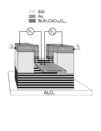
Figure 1: Sketch of the sample geometry used for injection experiments.

To realize this geometry the top layers of a larger mesa (structured as described above) had to be cut in two smaller ones. The whole sample was protected by electron-beam resist except a thin line on top of the big mesa. By etching this sample the larger mesa could be divided in two smaller mesas. To keep a part of the base below the two smaller ones the etching process had to be controlled precisely. The resistance of the gold lead was recorded during etching showing the time when gold was removed and separation of the big mesa began. With this technique we were able to structure samples with $5\times 10\mu m^{2}$ and $4\times 10\mu m^{2}$ mesas each including about 10 intrinsic Josephson junctions on top of one larger one ($10\times 10\mu m^{2}$, 6 junctions). The gap between the two top mesas was 1$\mu$m. All samples discussed in this article are listed in Tab. 1. The kind of experiments they are used for are marked by DM (double mesa) and FIR (FIR absorption).

Samples	area ($\mu m^{2}$)	$\#jj$	experiments
SR102_3	$10\times 10$ (B)	6	DM
	$4\times 10$ (M1)	10	DM
	$5\times 10$ (M2)	10	DM
SH104	$7\times 6$ (B)	11	DM
	$2\times 6$ (M1)	3	DM
	$3\times 4$ (M2)	4	DM
#32	$8\times 8$	8	FIR
#39	$10\times 10$	20	FIR
#20	$10\times 10$	11	FIR

Table 1: Table of samples described in this article. The area of the mesas and the number of junctions (#jj) containing it are listed together with the kind of experiments they were used for.

IV-characteristics of our samples were recorded by applying dc currents and recording voltages across mesas by digital voltmeters. If not mentioned otherwise all measurements were performed at a temperature of 4.2 K.

As radiation source for experiments presented in Section 4.1 we used a far-infrared laser which was optically pumped by a CO₂ laser. To minimize power losses we used a polyethylene lens producing a parallel beam. Inside the optical cryostat the samples were fixed in the center of a silicon hyperhemispherical lens to focus the radiation onto the mesa. Rother00 For some samples we used a very sensitive setup to detect Shapiro steps and to determine voltage of these resonances very precisely. For this purpose the laser beam was modulated by an optical chopper with a fixed frequency. With the chopper frequency as external reference, the voltage across the junction was connected to the input of a lock-in amplifier (LI). As the LI analyzes voltage changes occurring with the chopper frequency the output signal $V_{LI}$ exhibits a point-symmetric structure. Thus the LI output signal represents the voltage difference between IV- characteristics with and without laser radiation. The voltage of the Shapiro step can easily be identified as the symmetry point of this signal.

IV Experimental results

IV.1 Shapiro steps

Our experiments with high frequency electromagnetic radiation have been carried out with three samples #32 ($8\times 8\mu m^{2}$), #39 ($10\times 10\mu m^{2}$) and #20 ($10\times 10\mu m^{2}$). We first discuss results for sample #32 which consists of eight intrinsic Josephson junctions as can be seen in the IV-characteristics shown in Fig. 2.

Figure 2: IV characteristic of sample #32.

The increasing values of critical currents may be explained by the inhomogeneous etching process during fabrication producing layers with increasing areas from top to bottom of the mesa. Then it is natural to assume that the values of critical currents increase with the position of the junctions inside the mesa. In particular, the first resistive branch of the IV-characteristics should be assigned to the uppermost Josephson junction of the mesa. The critical current on branch number 0 is strongly suppressed and its IV-curve is linear, while the other branches show the typical non-linear IV-dependence characteristic for a tunneling junction between two superconducting layers with d-wave order parameter. The special behaviour of branch 0 might be explained by the assumption that the first superconducting layer is in proximity contact with the normal gold electrode.

This sample was irradiated with four external frequencies between 584 GHz and 762 GHz. On the IV characteristic we could detect first order Shapiro steps on the first resistive branch at an absolute voltage $V_{S}$ and current $I_{S}$. To compare the step-voltage with $hf/(2e)$ as predicted by the second Josephson relation the contact voltage $V_{0}(I)$ between Au leads and mesa in the superconducting state without radiation had to be measured. The value $\Delta V_{S}=V_{S}(I_{S})-V_{0}(I_{S})$ can then be compared with $hf/(2e)$. As shown in Fig. 3, $\Delta V_{S}$ evaluated for this sample is strictly lower than $hf/(2e)$ for all four frequencies. The relative shift is approximately $-3\%$.

This downshift can be explained if we assume that the Josephson junction in the resistive state which is locked to the external radiation with frequency $f$ is close to the normal electrode, i.e. between the first and second superconducting layer. For this junction we have

$$\frac{hf}{2e}=(1+2\alpha)V_{1,2}-\alpha(V_{0,1}+V_{2,3})+\Psi_{2}-\Psi_{1},$$ (12)

while for the other junctions, which are in the superconducting state, we use

$$0=(1+2\alpha)V_{n,n+1}-\alpha(V_{n-1,n}+V_{n+1,n+2})+\Psi_{n+1}-\Psi_{n}$$ (13)

for $n\geq 2$. Adding up these equations together with the current relation for the contact with the normal electrode (10) we obtain for the total voltage:

$$V_{S}=\frac{jd}{\sigma_{0,1}}+\frac{hf}{2e}.$$ (14)

Here we have assumed that $\Psi_{n}=0$ for $n\geq 3$. The contribution of $\Psi_{2}$ drops out. Finally, the charge-imbalance potential $\Psi_{1}$ vanishes on the first layer since the on- and off-flowing quasiparticle currents are equal, $j^{qp}_{0,1}=j^{qp}_{1,2}=j$.

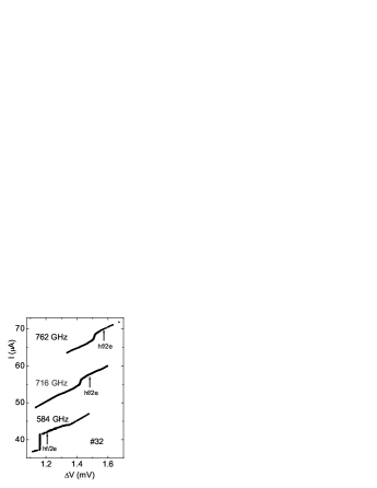
Figure 3: Voltages of Shapiro steps measured on IV characteristic of sample #32 compared to $hf/(2e)$ (for the higher frequencies the current axis is shifted).

We have to compare this result with the voltage measured in the absence of high-frequency irradiation, when all junctions are in the superconducting state. Then (13) holds for $n\geq 1$. Adding up now equations (13) and (10) we obtain for the total voltage (contact voltage in the superconducting state):

$$V_{0}=\frac{jd}{\sigma_{0,1}}+\Psi_{1}.$$ (15)

The quasi-particle potential on the first superconducting layer is now given by $\Psi_{1}=j\tau_{q}/(2e^{2}N(0))$ while $\Psi_{n}=0$ for $n\geq 2$. Subtracting the measured contact voltage from the voltage of the Shapiro step we obtain for the step-voltage:

$$\Delta V_{S}=\frac{\hbar\omega}{2e}-\delta V$$ (16)

with $\delta V=j\tau_{q}/(2e^{2}N(0))$. The shift is proportional to the life-time of charge-imbalance.

Figure 4: IV characteristic of sample #39.

Sample #39 consists of 20 intrinsic Josephson junctions. For this sample the distribution of critical currents is more homogeneous (Fig. 4) than for #32 making it impossible to determine the position of the junction generating the first resistive branch inside the mesa. By using the sensitive measurement technique with a pulsed laser beam we were able to detect Shapiro steps on the first resistive branch at three FIR frequencies between 1.40 THz and 1.63 THz. The voltage differences $\Delta V_{S}$ of these resonances were calculated as described above. In contrast to #32 for this sample no deviations from $hf/(2e)$ were measured. In view of the theory presented above this means, that the resistive junction which is locked to external radiation is not close to the normal electrode or the charge-imbalance time is rather short for this sample.

Finally we want to focus on sample #20 consisting of 11 intrinsic Josephson junctions. The IV-curves of this sample show a very homogeneous distribution of critical currents making it impossible to assign any branch to a junction at a certain position inside the mesa. However, for different current cycles (increase $I_{1}$ to its maximum value than decrease it zero) two different first branches marked 1a and 1b in Fig. 5 are measured. This means that two different junctions in the stack become resistive first.

We were able to detect Shapiro steps at five frequencies between 1.27 THz and 1.82 THz on both branches 1a and 1b. Analyzing the voltage differences $\Delta V_{S}$ we got different values for 1a and 1b (Fig. 6). On branch 1a the voltages of Shapiro steps were detected at regular values of $hf/(2e)$ whereas voltages of 1b were shifted to values $3\%$ below $hf/(2e)$. This behaviour can be explained by assuming that in case 1b the junction close to the normal electrode becomes resistive while in case 1a a junction inside the stack becomes resistive. This assumption is also in agreement with the observation that the voltage of the second branch at the critical current is approximately given by the sum of the voltages of 1a and 1b and the voltage differences for the higher branches are rather homogenous and are close to the value for branch 1a.

Figure 5: IV characteristic of #20. Several current cycles are shown in one figure.

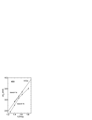
Figure 6: Voltages of Shapiro steps measured on IV characteristic of sample #20 compared to $hf/(2e)$. The values strongly depend on which branch 1a or 1b the resonances occured.

We want to mention that we could also measure Shapiro steps on higher resistive branches. Due to slightly varying parameters of different resistive Josephson junctions analysis of $\Delta V_{s,n}$ is much more complicated and was not accurate enough to deduce deviations from the second Josephson relation.

Finally we want to point out that a shift in the Shapiro step voltage is only possible, if the resistive junction is close to the normal electrode. In recent measurements of Shapiro steps in step-edge junctions Wang01 this is different. Here the resistive Josephson junction is inside a stack of superconducting layers and hence no shift is observed. Also no shift of Shapiro steps appears in true 4-point measurements and for steps crossing the zero-current line at the point of zero current. Doh00

IV.2 Injection experiments in double-mesa structures

The geometry of samples used for injection experiments in double-mesa structures is schematically shown in Fig. 1. As results obtained for the different samples are rather similar, we will discuss only results for sample #SR102_3. Here two small mesas M1 of lateral size $5\times 10\mu m^{2}$ and M2 of size $4\times 10\mu$m² were structured on a base mesa B of size $10m\times 10\mu m^{2}$. The currents $I_{1,2}$ through the mesas M1 and M2 and the base mesa B and the corresponding voltages $V_{1,2}$ can be measured separately. The brush-like structure of the IV-curves which is similar for the two mesas shows two sets of branches with different critical currents. These belong to 10 Josephson junctions in M1 and M2 and 6 junctions in the base mesa.

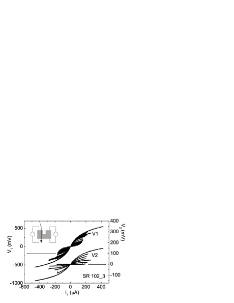
Figure 7: Voltages of M1 and M2 during variation of $I_{1}$ while $I_{2}=0$.

To explain the operation of the device we want to start with the case of no current flowing through M2 ($I_{2}=0$). Measuring $V_{1}$ and $V_{2}$ during variation of $I_{1}$ we obtained the curves shown in Fig. 7. $V_{1}(I_{1})$ shows the full set of IV-curves of M1 and B, while in $V_{2}(I_{1})$ only the resistive junctions of the base mesa B appear. Here $V_{2}(I_{1})$ is in fact a 4-point measurement of the IV-characteristic of the base mesa. Note that as long as the junctions in B are completely superconducting, the voltage $V_{2}$ is exactly zero and independent of $I_{1}$. If a small current $I_{2}$ is applied to M2, then $V_{2}(I_{2})$ shows the contact resistance between the gold electrode and the mesa. Again the voltage $V_{2}$ does not depend on $I_{1}$.

Now a larger bias current is applied to M2, such that some junctions of M2 are in the resistive state. Keeping $I_{2}$ fixed we varied the current $I_{1}$. During the cycling of $I_{1}$ junctions in M1 are switched on and off into the resistive state. From time to time also junctions in the other mesa M2 are switched on and off leading to discrete jumps in the voltage $V_{2}$, but otherwise $V_{2}$ is still constant (horizontal line in Fig. 8).

In some cases, however, the voltage on M2 jumps to an additional branch $V_{2}(I_{1})$, which splits off from the constant voltage branch and depends weakly on $I_{1}$. The jump into this branch, which is marked $\Delta V$ in Fig. 8, is always triggered by a switch into one of the higher order branches of M1. Let us note that this happens only if $I_{1}$ and $I_{2}$ are in opposite direction. In later cycles the branch $V_{2}(I_{1})$ can also traced out by increasing the current $I_{1}$ from zero. In general, several sets of voltage curves with split branches $\Delta V_{2}(I_{1})$ occur. The voltages of the horizontal branches correspond to different numbers of junctions of M2 beeing in the resistive state at the fixed current $I_{2}$. In Fig. 8 only the branch corresponding to two resistive junctions is shown.

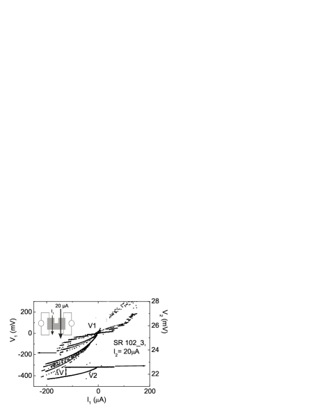
Figure 8: Voltages of M1 and M2 during variation of $I_{1}$ while two junctions of M2 are in the resistive state.

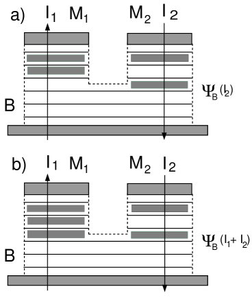
Figure 9: Charge-imbalance generated on the first layer of the base mesa by the currents through mesas M1 and M2.

The maximum voltage difference $\Delta V$ is much smaller than the voltage between different resistive branches in M2 at the bias current $I_{2}$. It is also much smaller than the voltage of resistive junctions in the base mesa. Therefore the appearence of $\Delta V_{2}(I_{1})$ must have a different origin and can be explained as follows: If the junctions between the lowest layers in both mesas M1 and M2 and the first common superconducting layer in B are resistive, then a nonequilibrium potential $\Psi_{B}$ is generated on the first superconducting layer of the base mesa. This is illustrated in Fig. 9: In Fig. 9a only the current $I_{2}$ contributes to the charge-imbalance potential, while in Fig. 9b both currents contribute. The generated charge-imbalance potential can be measured directly as additional voltage on M2:

$$\Delta V_{2}(I_{1})=\Psi_{B}(I_{1}+I_{2})-\Psi_{B}(I_{2}),$$ (17)

$$\Psi_{B}(I)=\frac{I}{A}\frac{\tau_{q}}{2e^{2}N(0)}.$$ (18)

Here $A$ is the area of the base mesa. In deriving (18) we assumed that the charge-imbalance relaxation time is large compared to the diffusion time of charge-imbalance along the layer.

Finally we want to explain the asymmetry of $V_{2}(I_{1})$ with respect to the polarity of both currents. The total current $I_{B}$ through B is either $I_{1}+I_{2}$ if the polarity is the same, or $I_{1}-I_{2}$ if the polarity is opposite. In the first case the total current through B is higher. This makes it possible that one junction inside B gets resistive before the critical current of the small mesas is exceeded. This destroys the precondition of a completely superconducting mesa B. When the polarity is opposite the current through B is always smaller than $I_{1}$ and junctions in M1 will get resistive before any junction in B.

IV.3 Determination of the charge-imbalance relaxation time

Both types of experiments can be used to measure the charge-imbalance relaxation time. From the shift of the Shapiro step we obtain

$$\tau_{q}=\delta V\frac{A}{I}2e^{2}N(0),$$ (19)

where $A$ is the area of the mesa. From the injection experiment in the double-mesa structure a similar expression is obtained. This equation contains the unknown density of states $N(0)$ of the two-dimensional electron gas at the Fermi surface. For a rough estimate we may use the density of states $N(0)=m/(2\pi\hbar^{2})$ of free conduction electrons with mass $m$, then $2e^{2}N(0)=0.67$C²J^-1m^-2. Alternatively, by using $\alpha=\epsilon\epsilon_{0}/(2e^{2}N(0)d)$ we can express $2e^{2}N(0)$ by the parameter $\alpha$, the dielectric constant $\epsilon$ of the barrier and the distance $d$ between superconducting layers. In Ref. Helm02, the values $\alpha=0.4$, $\epsilon=20$ have been estimated from reflectivity experiments (for another material). Here it is found that the value of $\epsilon\epsilon_{0}/(\alpha d)$ is rather close to the value of $2e^{2}N(0)$ calculated for free conduction electrons, which therefore will be used in the following.

With the data of sample #32: $A=64\mu$m², $I=30\mu$A, $\delta V=50\mu$V we find $\tau_{q}\simeq 70$ ps. An estimate for the shifts on branch 1b of sample #20 with 1.63 THz gives values of $\tau_{q}\simeq$ 450 ps. In a similar way we can also determine $\tau_{q}$ from the injection experiments in double-mesa structures. Using $I_{1}=120\mu$A, $I_{2}=20\mu$A, $\Delta V=0.6$mV, $A=100\mu$m² we find $\tau_{q}\simeq$ 330 ps, which is similar to the values obtained from the shifts of Shapiro steps.

The charge-imbalance relaxation time $\tau_{q}$ describes the recombination of quasi-particles into Cooper pairs. It should be distinguished from the characteristic time for the thermalisation of hot quasi-particles, which is much shorter. Nessler98 Note that in the present case $\tau_{q}$ is much longer than the period of a Josephson oscillation on a Shapiro step. For the charge-imbalance relaxation normally inelastic phonon scattering processes are responsible. It should be noted that in the case of d-wave pairing with an anisotropic gap also elastic impurity scattering contributes. Tinkham96

V Summary

In this paper we have discussed new experiments showing evidence of non-equilibrium effects in intrinsic Josephson contacts in layered superconductors, which are due to charge-imbalance produced by a stationary bias current. In particular, we have investigated the voltage-position of Shapiro steps in the presence of high-frequency irradiation. In some cases we observed a down-shift of 3% from the canonical value of $hf/(2e)$. This shift, which is not a violation of the basic Josephson relation, can be explained by charge imbalance on the first superconducting layer if the Josephson contact is next to the normal electrode.

In another type of experiment we studied the mutual influence of currents through two mesas on a common base mesa on the measured voltages. The reults can be explained by charge-imbalance on the first common superconducting layer of the base mesa. This experiments has some similarity with the classical experiment by Clarke, Clarke72 where charge imbalance is produced in a superconductor by a strong quasi-particle current which is then detected as voltage difference between a normal contact and a Josephson contact.

Both experiments allow to measure the charge-imbalance relaxation time which is of the order of 100 ps.

References

- (1) R. Kleiner, F. Steinmeyer, G. Kunkel, and P. Müller, Phys. Rev. Lett. 68, 2394 (1992)
- (2) R. Kleiner and P. Müller, Phys. Rev. B 49, 1327 (1994); P. Müller in: Festkörperprobleme/Advances in Solid State Physics, Vol 34, ed. by Helbig R (Vieweg, Braunschweig), 1 (1994)
- (3) A. Yurgens, D. Winkler, N.V. Zavaritsky, T. Claeson, Phys. Rev. 53, R8887 (1996);
- (4) T. Koyama and M. Tachiki, Phys. Rev. B 54, 16183 (1996).
- (5) L.N. Bulaevskii, D. Dominguez, M.P. Maley, A.R. Bishop, and B.I. Ivlev, Phys. Rev. B 53, 14601 (1996).
- (6) S.N. Artemenko and A.G. Kobelkov, Phys. Rev. Lett. 78, 3551 (1997).
- (7) D.A. Ryndyk, Phys. Rev. Lett. 80, 3376 (1998).
- (8) C. Preis, C. Helm, J. Keller, A. Sergeev, and R. Kleiner, in Superconducting Superlattices II: Native and Artificial, I. Bozovic and D. Pavona, editors, Proceedings of SPIE Volume 3480, 236 (1998).
- (9) S.E. Shafranjuk, M. Tachiki, Phys. Rev. B 59, 14087 (1999).
- (10) D.A. Ryndyk, JETP 89, 975 (1999), [Zh. Eksp. Teor. Fiz. 116, 1798 (1999)].
- (11) C. Helm, J. Keller, C. Preis, and A. Sergeev, Physica C 362 43 (2001).
- (12) D.A. Ryndyk, J. Keller and C. Helm, J. Phys.: Condens. Matter 14, 815 (2002).
- (13) C. Helm, L.N. Bulaevskii, E.M. Chudnovsky, M.P. Maley, Phys. Rev. Letters, 89, 057003 (2002).
- (14) L.N. Bulaevskii, C. Helm, A.R. Bishop, M.P. Maley, Europhys. Lett. 58 415 (2002; C. Helm, L.N. Bulevskii, cond-math/0207491, submitted to Phys. Rev. B
- (15) J. Clarke, Phys. Rev. Lett. 28, 1363 (1972); M. Tinkham, J. Clarke, Phys. Rev. Lett. 28, 1366 (1972).
- (16) A. Schmid, G. Schön, J. Low Temp. Phys. 31, 1 (1975).
- (17) M.Tinkham, Introduction to Superconductivity, second edition, McGraw-Hill (1996), Chapter 11.
- (18) S. Rother, R. Kleiner, P. Müller, Y. Kasai, K. Nakajima, Physica C 341-348 1565 (2000; S. Rother, Y. Koval, P. Müller, R. Kleiner, Y. Kasai, K. Nakajima, M. Darula, IEEE Trans. Appl. Superconductivity 11, 1191 (2001)
- (19) H.B. Wang, P.H. Wu, T. Yamashita, Phys. Rev. Lett. 87, 107002 (2001); H.B. Wang, L.X. You, J. Chen, P.H. Wu, T. Yamashita, Supercond. Sci. Technol. 15 90 (2002)
- (20) Y.J. Doh, J. Kim, K.T. Kim, and H.J. Lee, Phys. Rev. B 61, R3834 (2000).
- (21) W. Nessler, S. Ogawa, H. Nagano, H. Petek, J. Shimoyama, Y. Nakayama, K. Kishio, Phys. Rev. Lett. 81, 4480 (1998)