Coherent resistance of a disordered 1D wire: Expressions for all moments and evidence for non-Gaussian distribution

Abstract

We study coherent electron transport in a one-dimensional wire with disorder modeled as a chain of randomly positioned scatterers. We derive analytical expressions for all statistical moments of the wire resistance $\rho$. By means of these expressions we show analytically that the distribution $P(f)$ of the variable $f=\ln(1+\rho)$ is not exactly Gaussian even in the limit of weak disorder. In a strict mathematical sense, this conclusion is found to hold not only for the distribution tails but also for the bulk of the distribution $P(f)$.

I Introduction

It is known that a coherent electron wave in a disordered one-dimensional (1D) wire of infinite length is exponentially localized by an arbitrary weak disorder. Mott-61 ; Borland-61 ; Mott-90 The resistance $\rho$ of the 1D wire of length $L$ should therefore increase with $L$ exponentially. In fact, the resistance wildly fluctuates from wire to wire in an ensemble of macroscopically identical wires (with disorder in each wire being microscopically different) and what increases exponentially is the mean resistance and also the “typical” resistance. Landauer-70 ; Anderson-80

It has also become clear that the resistance $\rho$ is not a self-averaged quantity. Anderson-80 In fact, the resistance fluctuations are so huge that (i) the resistance dispersion exceeds the mean resistance many orders of magnitude, (ii) the higher moments of the resistance exceed the mean resistance even more drastically, and (iii) the mean resistance is much larger than the typical one. These features are due to the fact that the moments of $\rho$ are governed by extremely high resistances occurring with an extremely low (but nonzero) probability.

To avoid the absence of self-averaging, the distribution $P(f)$ of the variable $f=\ln(1+\rho)$ was studied instead of the distribution $P(\rho)$.Anderson-80 ; stare ; Melnikov ; Shapiro-87 In contrast to $P(\rho)$, distribution $P(f)$ is well localized around the mean value $\overline{f}$. It is commonly accepted that for long enough wires the bulk of the distribution $P(f)$ is described by the Gauss function

$$P(f)=\frac{1}{\sqrt{2\pi\Delta^{2}}}\exp\left[-\frac{{(f-\bar{f})}^{2}}{2\Delta^{2}}\right],$$ (1)

where $\Delta^{2}\equiv\overline{f^{2}}-{\overline{f}}^{2}$ is the variance, while the tails of the distribution $P(f)$ are allowed to be non-universal and depend on the model of disorder. In the limit of weak disorder it is accepted that $\Delta^{2}=2\overline{f}$, i.e., that the distribution (1) obeys the single parameter scaling. The two-parameter scaling is accepted to appear for strong disorder, where $\Delta^{2}$ is not an unambiguous function of $\overline{f}$. crs Interesting to note, the authors of Ref. deych, found two-parameter scaling also for weak disorder, namely for the Anderson 1D disorder at certain conditions.

In this paper we study coherent transport in a 1D wire with disorder modeled as a chain of randomly positioned scatterers. We derive analytically all statistical moments of the wire resistance. By means of these moments we prove in the limit of long wires, that the distribution $P(f)$ always deviates from the Gauss distribution. The form of $P(f)$ for $f>\overline{f}$ is concluded to be nonuniversal (dependent on the model of disorder) even in the limit of weak disorder. In other words, in realistic wires disorder is never weak enough for $P(f)$ to be exactly Gaussian. The only approximation of our analysis is the phase randomization hypothesis. We confirm its validity by numerical simulations.

In Sec. II we specify two different model of disordered 1D wire. As a model I we consider the statistical ensemble of wires with the same number of scatterers in each wire, in the model II we let the number of scatterers to fluctuate from wire to wire. In Sec. III the moments of the wire resistance are derived for both models analytically assuming the phase randomization hypothesis. This hypothesis is verified in Sect. IV by means of numerical simulations. In Sec. V we prove that our expressions for the resistance moments are not consistent with the Gaussian form of $P(f)$ even in the limit of weak disorder. Discussion is given in Sect. VI.

II Model of disordered 1D wire

We consider a 1D wire with disorder represented by random potential

$$V(x)=\sum_{i=1}^{N}\gamma\delta(x-x_{i}),$$ (2)

where $\gamma\delta(x-x_{i})$ is the $\delta$-shaped impurity potential of strength $\gamma$, $x_{i}$ is the $i$-th impurity position selected at random along the wire, and $N$ is the number of impurities in the wire. Since the positions $x_{i}$ are mutually independent, the distances $a=x_{i+1}-x_{i}$ between the neighboring impurities follow the distribution $P(a)=N_{I}\exp[-N_{I}a]$, where $N_{I}$ is the 1D density of impurities and $N_{I}^{-1}$ is the mean distance between the neighboring impurities.

In the following sections we examine two models. In the model I we consider the statistical ensemble of wires with $N$ fixed in each wire to its mean value $\langle N\rangle$. In the model II we fix the wire length $L$ and we let $N$ to fluctuate from wire to wire according to the distribution

$${\mathcal{G}}(N)=\langle N\rangle^{N}e^{-\langle N\rangle}/N!.$$ (3)

It is easy to show that this distribution follows from the distribution $P(a)$. In both models $\langle N\rangle\equiv LN_{I}$.

The wire resistance $\rho$ (in units $h/2e^{2}$) is given by the Landauer formula Landauer-70

$$\rho=\frac{R(\varepsilon_{F})}{T(\varepsilon_{F})},$$ (4)

where $R$ and $T$ are the reflection and transmission coefficients describing the electron tunneling through disorder at the Fermi energy.

Using eq. (4) we follow a number of previous localization practitioners. Instead of eq. (4) we could use the two-terminal resistance $\rho=1/T=R/T+1$, which involves an extra term (unity on the right hand side) representing the fundamental resistance of contacts. The resistance (4) thus represents the resistance of disorder, directly measurable only by four-probe techniques. The problem is that eq. (4) ignores the effect of measurement probes Landauer-90 ; Datta-95 . We wish to note that this is not a serious problem in our case. First, we examine the regime $R/T\gg 1$, for which the two-terminal resistance $\rho=R/T+1$ coincides with eq. (4). Second, with $\rho=R/T+1$ we would arrive at the same conclusions as with eq. (4). Third, in principle, one can measure $R/T$ indirectly, by measuring the two-terminal resistance and then subtracting unity.

For disorder (2) both $R$ and $T$ can be obtained by solving the tunneling problem

$$\left[-\frac{\hbar^{2}}{2m}\ \frac{d^{2}}{dx^{2}}+V(x)\right]\Psi_{k}(x)=\mathcal{E}\Psi_{k}(x)$$ (5)

with boundary conditions

$$\Psi_{k}\left(x\rightarrow 0\right)=e^{ikx}+r_{k}e^{-ikx},~{}~{}~{}\Psi_{k}\left(x\rightarrow L\right)=t_{k}e^{ikx},$$ (6)

where $\mathcal{E}=\hbar^{2}k^{2}/2m$ is the electron energy, $m$ is the effective mass, and $r_{k}$ and $t_{k}$ are the reflection and transmission amplitudes. The coefficients $R={|r_{k}|}^{2}$ and $T={|t_{k}|}^{2}$ need to be evaluated at the Fermi wave vector $k=k_{F}$.

The reflection coefficient of a single $\delta$-barrier is given as $R_{I}=\Omega^{2}/(k_{F}^{2}+\Omega^{2})$, where $\Omega=m\gamma/\hbar^{2}$. We fix

$$k_{F}=7.9\times 10^{7}{\text{m}}^{-1}$$ (7)

and $m=0.067m_{0}$, and we parameterize the $\delta$-barrier by $R_{I}$. We ignore the fluctuations of $R_{I}$ as well as the spread of the impurity potentials.

III Resistance moments

III.1 Model I

We start with derivation of the mean resistance. Assume that we know the reflection coefficient $R_{N}$ of a specific configuration of $N$ randomly positioned impurities. If we add to this configuration an extra impurity at position $x_{N+1}$, we can express $R_{N+1}$ through $R_{N}$ and $R_{I}$. It is useful to express $R_{N+1}$ in the form Landauer-70

$$\frac{R_{N+1}}{1-R_{N+1}}=\frac{R_{N}+R_{I}-2\sqrt{R_{N}R_{I}}\cos\phi_{N}}{(1-R_{N})(1-R_{I})},$$ (8)

where $\phi_{N}$ is the phase specified below. Writing eq. (8) in terms of the wire resistance

$$\rho_{N}\equiv\frac{R_{N}}{1-R_{N}}$$ (9)

and in terms of

$$\lambda_{1}\equiv\frac{1+R_{I}}{1-R_{I}}$$ (10)

we get

$$\rho_{N+1}=\lambda_{1}\rho_{N}+\frac{\lambda_{1}-1}{2}-\sqrt{(\lambda_{1}^{2}-1)(\rho_{N}+\rho^{2}_{N})}\cos\phi_{N}.$$ (11)

The phase $\phi_{N}=2k_{F}a+\phi_{0}$, where $a=x_{N+1}-x_{N}$ is the inter-impurity distance, and $\phi_{0}$ is the ($a$-independent) phase due to the reflection by the obstacles. Landauer-70 ; Anderson-80 Obviously,

$$\rho_{0}\equiv 0$$ (12)

and

$$\rho_{1}\equiv\frac{R_{I}}{1-R_{I}}=\frac{\lambda_{1}-1}{2}.$$ (13)

Note that $\rho_{2}$ depends on $\phi_{1}$, $\rho_{3}$ depends on $\phi_{2}$ and $\phi_{1}$, etc., $\rho_{N+1}$ thus depends on $\phi_{N}$, $\phi_{N-1}$, $\dots$, $\phi_{2}$, and $\phi_{1}$.

If we assume that $a\gg 2\pi/k_{F}$, then $\phi_{N}$ changes rapidly with $a$ and fluctuates at random from sample to sample as $a$ fluctuates. The ensemble average of $\rho_{N+1}$ over the inter-impurity distance $x_{N+1}-x_{N}$ then simplifies to Landauer-70 ; Anderson-80

$$\overline{\rho_{N+1}}=\frac{1}{2\pi}\,\int\limits_{0}^{2\pi}d\phi_{N}\,\rho_{N+1}.$$ (14)

If we average eq. (11) over $\phi_{N}$, the term $\propto\cos\phi_{N}$ becomes zero. If we then average over $\phi_{N-1}$, …, $\phi_{2}$, $\phi_{1}$, we obtain the recursion equation

$$\overline{\rho_{N+1}}=\lambda_{1}\overline{\rho_{N}}+\frac{1}{2}(\lambda_{1}-1).$$ (15)

We solve Eq. (15) with initial condition (12) and obtain the mean resistance

$$\overline{\rho_{N}}=\frac{1}{2}\left(\lambda_{1}^{N}-1\right).$$ (16)

The higher moments can be obtained in the same way. The $m$th power of eq. (11) averaged over $\phi_{N}$ formally reads

$$\overline{\rho^{m}_{N+1}}=\overline{\left[\lambda_{1}\rho_{N}+\frac{\lambda_{1}-1}{2}-\sqrt{(\lambda_{1}^{2}-1)(\rho_{N}+\rho^{2}_{N})}\cos\phi_{N}\right]^{m}}.$$ (17)

If we take into account that AS

$$\frac{1}{2\pi}\int\limits_{0}^{2\pi}d\phi\left(\cos\phi\right)^{2m}=\frac{1}{2^{2m}}\binom{2m}{m}$$ (18)

and

$$\frac{1}{2\pi}\int\limits_{0}^{2\pi}d\phi\left(\cos\phi\right)^{2m-1}=0,$$ (19)

we easy see that eq. (17) takes the form

$$\overline{\rho_{N+1}^{m}}=\sum_{k=0}^{m}\alpha_{k}(m)\rho_{N}^{k},$$ (20)

where coefficients $\alpha_{k}(m)$ are polynomial functions of $\lambda_{1}$. Averaging each $\rho_{N}^{k}$ over $\phi_{N-1}$, each $\rho_{N-1}^{k}$ over $\phi_{N-2}$, etc., we finally obtain the recursion relation

$$\overline{\rho_{N+1}^{m}}=\sum_{k=0}^{m}\alpha_{k}(m)\overline{\rho_{N}^{k}}.$$ (21)

A general expression for coefficients $\alpha_{k}(m)$ is given in the Appendix A, where we also derive

$$\alpha_{m}(m)=\overline{\left[\lambda_{1}-\sqrt{\lambda_{1}^{2}-1}\cos\phi\right]^{m}}.$$ (22)

We can also obtain eq. (22) by comparing the right hand sides of Eqs. (17) and (20) for $\rho_{N}\to\infty$, where they reduce to $\overline{[\lambda_{1}-\sqrt{\lambda_{1}^{2}-1}\cos\phi]^{m}}\rho_{N}^{m}$ and $\alpha_{m}(m)\rho_{N}^{m}$, respectively.

We solve Eq. (21) recursively. Suppose that the $N$-dependence of $\overline{\rho^{m}_{N}}$ can be expressed in the form

$$\overline{\rho_{N}^{m}}=a_{m}(m)\lambda_{m}^{N}+\dots a_{1}(m)\lambda_{1}^{N}+a_{0}(m).$$ (23)

For $m=1$ eq. (23) coincides with eq. (16). Therefore, $\lambda_{1}$ in eq. (23) coincides with eq. (10) and $a_{1}(1)=1/2$, $a_{0}(1)=-1/2$. Once we know $\lambda_{1}$, $a_{1}(1)$, and $a_{0}(1)$, we can solve the problem for $m=2$ and determine $\lambda_{2}$, $a_{2}(2)$, $a_{1}(2)$, and $a_{0}(2)$ (see the Appendix B). Generally, once we determine all $\lambda_{k}$ and all coefficients $a_{n}(k)$ for $0\leq n\leq k\leq m-1$, we can insert expansion (23) into eq. (21) and compare the $N$-independent factors at all $\lambda_{k\leq m}^{N}$. This gives us linear equations

$$a_{k}(m)\lambda_{k}=\sum\limits_{i=k}^{m}\alpha_{i}(m)\,a_{k}(i)$$ (24)

for all $a_{k}(m)$ with $k<m$ and in addition the identity $\lambda_{m}\equiv\alpha_{m}(m)$, i.e.,

$$\lambda_{m}=\overline{\left[\lambda_{1}-\sqrt{\lambda_{1}^{2}-1}\cos\phi\right]^{m}}.$$ (25)

As a last step we calculate the coefficient $a_{m}(m)$ with help of the initial condition (12). In the Appendix B this procedure is demonstrated in detail for $m=2$. The result is

$$\overline{\rho_{N}^{2}}=\frac{1}{6}\lambda_{2}^{N}-\frac{1}{2}\lambda_{1}^{N}+\frac{1}{3},$$ (26)

where

$$\lambda_{2}=\frac{1}{2}\left(3\lambda_{1}^{2}-1\right).$$ (27)

Parameters $\lambda_{k}$ characterize the exponential increase of $\overline{\rho^{m}_{N}}$ with $N$. Equation (25) expresses $\lambda_{k}$ analytically for arbitrary $k$, for example, for $m=1$ and $2$ it reproduces relations (10) and (27), respectively. We present also

$$\lambda_{3} = \frac{5}{2}\,\lambda_{1}^{3}-\frac{3}{2}\,\lambda_{1},$$ (28)

$$\lambda_{4} = \frac{35}{8}\,\lambda_{1}^{4}-\frac{15}{4}\,\lambda_{1}^{2}+\frac{3}{8},$$ (29)

$$\lambda_{5} = \frac{63}{8}\,\lambda_{1}^{5}-\frac{35}{4}\,\lambda_{1}^{3}+\frac{15}{8}\,\lambda_{1},$$ (30)

$$\lambda_{6} = \frac{231}{16}\,\lambda_{1}^{6}-\frac{315}{16}\,\lambda_{1}^{4}+\frac{105}{16}\,\lambda_{1}^{2}-\frac{5}{16}.$$ (31)

We do not present explicitly complete expressions for moments $\overline{\rho_{N}^{m}}$ higher than $\overline{\rho_{N}^{2}}$. For further purposes we only express the leading term of $\overline{\rho_{N}^{m}}$. We see from (25) that $\lambda_{1}<\lambda_{2}<\dots<\lambda_{m}$. Therefore, for large enough $N$

$$\overline{\rho^{m}_{N}}\approx a_{m}(m)\,\lambda_{m}^{N}\propto\lambda_{m}^{N}.$$ (32)

For completeness, we derive also the mean value of the variable $f$. As in Ref. Anderson-80, , we average over all phases the variable $f_{N}=\ln\left(1+\rho_{N}\right)$ and obtain the recursion relation $\overline{f_{N+1}}=-\ln(1-R_{I})+\overline{f_{N}}$. We solve this equation with the condition $\rho_{0}\equiv 0$ (i.e, with $\overline{f}_{0}\equiv 0$) and obtain

$$\overline{f_{N}}=-N\ln(1-R_{I}).$$ (33)

No simple analytic expressions exist for higher moments $\overline{f^{m}}$. For details see Refs. Anderson-80, ; stare, ; crs, .

III.2 Model II

In the preceding section the number of impurities, $N$, was kept at the same value for each wire in the wire ensemble (model I). In this section we let $N$ to fluctuate from wire to wire according to the distribution (3) while keeping for each wire the same wire length $L$ (model II). Thus, to obtain the resistance moments for the model II we just need to average over the distribution (3) the moments obtained in the preceding section. In particular,

$$\langle\lambda^{N}_{m}\rangle=\sum_{N=1}^{\infty}\lambda_{m}^{N}\mathcal{G}_{N}=e^{(\lambda_{m}-1)N_{I}L}=e^{m(m+1)L/\xi_{m}},$$ (34)

where we define the $m$th characteristic length $\xi_{m}$ as

$$\xi_{m}^{-1}=\frac{N_{I}\left(\lambda_{m}-1\right)}{m(m+1)}.$$ (35)

From Eqs. (16,34) we obtain the mean resistance

$$\overline{\rho}=\frac{1}{2}(e^{2L/\xi_{1}}-1)$$ (36)

and from Eqs. (26,34) the 2nd moment

$$\overline{\rho^{2}}=\frac{1}{6}e^{6L/\xi_{2}}-\frac{1}{2}e^{2L/\xi_{1}}+\frac{1}{3}.$$ (37)

The typical resistance is defined as $\rho_{t}=\exp{\overline{f}}-1$. We average $\overline{f}$ (eq. 33) over the distribution (3) and obtain

$$\rho_{t}=\exp{L/\xi}-1,$$ (38)

where

$$\xi^{-1}=-N_{I}\ln(1-R_{I})=N_{I}\ln\left(\frac{\lambda_{1}+1}{2}\right).$$ (39)

is the electron localization length. For comparison,

$$\xi_{1}^{-1}=N_{I}\frac{R_{I}}{1-R_{I}}=N_{I}\left(\frac{\lambda_{1}-1}{2}\right).$$ (40)

It is easy to show comments that $L/\xi_{m}$ can be expressed as an unambiguous function of $L/\xi$ a $L/\xi_{1}$. This means that our models exhibit two-parameter scaling. Only if $R_{I}$ is very small, both lengths converge to the same limit

$$\xi\approx\xi_{1}\approx{(N_{I}R_{I})}^{-1}\quad,\quad R_{I}\ll 1.$$ (41)

However, $\xi\neq\xi_{1}$ for any nonzero $R_{I}$.

IV Microscopic modeling

Our derivation of resistance moments relies on the phase randomization hypothesis, i.e., on the averaging (14). This should be justified in the limit $a\gg 2\pi/k_{F}$, that means for $1/N_{I}\gg 2\pi/k_{F}$. Now we test the phase randomization hypothesis by microscopic modeling.

Figure 1: Distribution $P(\phi)$ for various model parameters.

In our microscopic model we select disorder as discussed in Sect. II, solve Eq. (5) by the transfer matrix method, transfermatrix and obtain from Eq. (4) the resistance of a single wire. We repeat this process for a statistical ensemble of wires typically involving $10^{6}$ - $10^{9}$ samples.

In Fig. 1 we present the distribution $P(\phi)$ of the variable $\phi$, where $\phi$ is the phase entering the right hand side of eq. (11). The distribution $P(\phi)$ can be accumulated either within the ensemble of wires with just two randomly positioned impurities within each wire, or within a single wire into which many impurities are positioned one by one. Both procedures give the same results.

In accord with the phase randomization hypothesis (14), for low impurity density $N_{I}$ (left panel) we see that $P(\phi)\approx$ const = $1/(2\pi)$. Note that the flat distribution survives for rather large $R_{I}$ values. On the other hand, when $N_{I}$ is large, it tends to destroy the flatness of $P(\phi)$ even for very small values of $R_{I}$ (right panel).

Results presented in Fig. 1 are consistent with those in Fig. 2 where the mean and typical resistances obtained by microscopic modeling are presented for various reflection coefficients $R_{I}$ and various densities $N_{I}$. For low $N_{I}$ our microscopic data agree well with our analytical results. Note that this is the case also for large $R_{I}$. However, with increasing $N_{I}$ the agreement deteriorates.

V Moments of the resistance in the limit of very long wires.

In the limit of long wires $\langle N\rangle$ becomes large and only the leading term of the moment $\overline{\rho^{m}_{N}}$ becomes important. From Eqs. (32) and (34) one easy obtains

$$\overline{\rho^{m}}\propto\left\{\begin{array}[]{ll}\lambda_{m}^{\langle N\rangle}&~{}~{}\text{Model~{}I}\\ {}{}{}&{}{}{}\\ e^{\langle N\rangle(\lambda_{m}-1)}&~{}~{}\text{Model~{}II}\end{array}\right.$$ (42)

From Eq. 25 it is evident that

$$\ln\lambda_{m}\approx m~{}~{}~{}~{}~{}~{}~{}m\gg 1$$ (43)

In Fig. 3 the estimate (43) is verified numerically. Using eq. (43) and $\langle N\rangle\equiv LN_{I}$ we can obtain from (42)

$$\ln\overline{\rho^{m}(L)}\propto\left\{\begin{array}[]{ll}mL&~{}~{}\text{Model~{}I}\\ \\ Le^{m\eta}&~{}~{}\text{Model~{}II}\end{array}\right.$$ (44)

Now we show that the analytical formulae (44) are not consistent with the assumption that the distribution $P(f)$ is Gaussian. To see this clearly, let us average the $m$th power of the resistance

$$\overline{\rho^{m}(L)}=\int_{0}^{\infty}df\ P(f)(e^{f}-1)^{m}$$ (45)

over the Gauss distribution (1). The result can easy be obtained analytically as

$$\overline{\rho^{m}(L)}=\sum_{k=1}^{m}(-1)^{m-k}\binom{m}{k}\exp\left(\frac{k^{2}\Delta^{2}}{2}+k\bar{f}\right).$$ (46)

In the limit $L/\xi\gg 1$ relation (46) reduces to

$$\overline{\rho^{m}(L)}=\exp\left(\frac{m^{2}\Delta^{2}}{2}+m\overline{f}\right).$$ (47)

Since $\Delta^{2}\propto L$, from (47)we have

$$\ln\overline{\rho^{m}(L)}\propto m^{2}L.$$ (48)

In particular, for weak disorder $\Delta^{2}=2\bar{f}=2L/\xi$ and the leading term in the sum (46) reads $\propto e^{m(m+1)L/\xi}$.

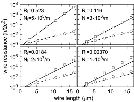
Figure 2: Mean resistance (squares, full lines) and typical resistance (circles, dashed lines) versus the wire length $L$. Squares and circles are the microscopic model results, full lines and dashed lines are graphic representation of the formulas (36) and (38), respectively. $k_{F}$ is given in Eq. 7. Parameters $N_{I}$ and $R_{I}$ are varied in such way that the localization length is the same ($\xi=2.7$ $\mu$m) for each panel. The accuracy of Eqs. (36) and (38) deteriorates with increasing $N_{I}$.

If we compare eq. (48) with our analytical results (44), we immediately see that relations (44) do not approach the dependence $\propto m^{2}L$ predicted by relation (48). Since the higher moments of the resistance are mainly governed by the distribution $P(f)$ for $f>\overline{f}$, the difference between the relations (48) and (44) is a proof that $P(f)$ deviates from the Gauss distribution in the model I as well as in the model II.

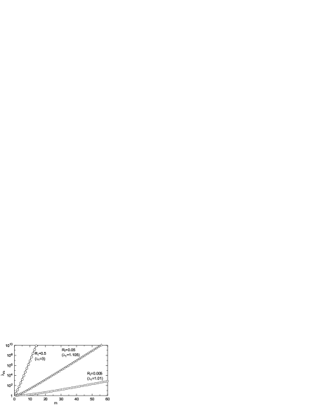
Figure 3: $m$-dependence of $\ln\lambda_{m}$ for various $R_{I}$.

It is important to note that these deviations are not restricted to the distribution tail $f\gg\overline{f}$. It is known that the tail of the distribution $P(f)$ is non-universal. From Eq. (11) we see that $\rho_{N+1}\leq(\lambda_{1}+\sqrt{\lambda_{1}^{2}-1})\rho_{N}$. Therefore, in the model I the value of $f$ never exceeds the maximum value $f_{\text{max}}$ given by

$$\frac{f_{\text{max}}}{\overline{f}}\approx\frac{\ln\left(\lambda_{1}+\sqrt{\lambda_{1}^{2}-1}\right)}{\ln\left[(\lambda_{1}+1)/2\right]}.$$ (49)

Due to this reason, in the model I the distribution $P(f)$ drops to zero for $f>f_{\text{max}}$ and some deviations from the Gauss distribution (1) can be expected to appear already for $f$ slightly below $f_{\text{max}}$. The same holds also for the model II in which $N$ fluctuates so that the difference $f_{\text{max}}(\text{model II})-f_{\text{max}}(\text{model I})$ is of order of $\sqrt{N}$. This means that the distribution $P(f)$ drops to zero in both models if $f$ is large enough.

However, this sudden drop to zero is not responsible for the nonGaussian behavior represented by eq. (44). To prove this we now show that $\overline{\rho^{m}}$ is governed by the $f$ values much smaller that $f_{\text{max}}$. We show that the maximum of the function $P(f)\times e^{mf}$ is positioned at $f=f_{m}$, where $f_{m}$ is much smaller than $f_{\text{max}}$. For the Gaussian distribution (1) we find

$$\frac{f_{m}}{\overline{f}}=\frac{\overline{f}+m\Delta^{2}}{\overline{f}}=(2m+1).$$ (50)

This ratio depends neither on $L$ nor on $\lambda_{1}$. Note that the ratio $f_{\text{max}}/\overline{f}$ does not depend on $L$ but it still depends on $\lambda_{1}$. In the limit of weak disorder ($R_{I}\to 0$) we obtain $\lambda_{1}\approx 1+2R_{I}$ and $f_{\text{max}}/\overline{f}\sim 2/\sqrt{R_{I}}\to\infty$. It is thus evident that $f_{m}\ll f_{\text{max}}$ at least in the limit of weak disorder.

From (44) we obtain

$$\frac{\ln\overline{\rho^{m+1}(L)}}{\ln\overline{\rho^{m}(L)}}=\frac{m+1}{m}$$ (51)

for the model I, while for the Gaussian distribution

$$\frac{\ln\overline{\rho^{m+1}(L)}}{\ln\overline{\rho^{m}(L)}}=\frac{m+2}{m}$$ (52)

This proves that $P(f)$ deviates the Gaussian distribution already for $f$ from the neighbourhood of $f_{1}$. As discussed above, this region is still far from the distribution tail.

In the model II this deviation from the Gaussian shape is even more pronounced, because $\overline{\rho^{m}(L)}$ increases with $m$ much faster than the dependence (47). This means that $P(f)$ decreases for $f>\overline{f}$ much slower than the Gaussian distribution. The slower decrease means that the deviation from Gaussian is surely not caused by the cutoff at $f=f_{\text{max}}$.

VI Discussion and conclusions

In conclusion, we have presented two simple models of disordered wire which allowed us to express analytically all moments of the wire resistance. By means of these analytical expressions we have succeeded to prove analytically the nonGaussian behavior of the distribution $P(f)$.

Analytical formulae for the resistance moments were obtained assuming the phase randomization hypothesis. In Sect. IV we have proven numerically that this hypothesis is indeed valid for small impurity density $N_{I}$. This means that for small enough $N_{I}$ our results are exact.

In fact, in a strict mathematical sense there is no single parameter scaling in the models I and II, because the lengths $\xi$ and $\xi_{1}$ always differ from each other. The difference between them is very small in the limit of small reflection coefficient, $R_{I}\ll 1$. Then, numerical experiment is not able do distinguish between $\xi$ and $\xi_{1}$ and the single parameter scaling holds to a good approximation for the bulk of the distribution.

If we accept $\xi=\xi_{1}$ as in eq. (41), then the relations (36), (37) and (38) agree with those derived within the scaling theory of localization. stare Note that the relation (41) is exact only if the second and higher orders of $R_{I}$ can be neglected. The same condition assures the equivalence of eq. (48) with eq. (44). Indeed, if we expand $\lambda_{m}$ [eq. (25)] into powers of $R_{I}$ and neglect all higher powers of $R_{I}$, we can interpret the obtained “expansion” as the first two terms of the Taylor expansion of the exponential function, i.e.,

$$\lambda_{m}=1+m(m+1)R_{I}+\mathcal{O}(R_{I}^{2})\approx e^{\left[m(m+1)R_{I}\right]}.$$ (53)

We show in Fig. 4 that the approximation (53) is very good in the limit of very small $R_{I}$ and small $m$. However, for any $R_{I}$ we can find such $m$ that the approximation (53) is no longer valid. Therefore, relation (48) does not give the correct $R_{I}$ dependence for higher moments of resistance. This proves that the distribution $P(f)$ is not Gaussian even for an infinitesimally small $R_{I}$.

Figure 4: The ratio $\lambda_{m}/\exp\left[m(m+1)R_{I}\right]$ as a function of $R_{I}$ for $m=$1 – 5.

The main difference between the presented results and those of the scaling theory of localization is that in our model we keep the exact $R_{I}$ dependence of all $\lambda_{m}$s while in the scaling theory only the linear term in $R_{I}$ is kept. To understand this difference more clearly, let us go back to the relation (15). We can approximate $\lambda_{1}$ as in (53) and rewrite (15) as

$$\overline{\rho_{N+1}}=\delta\rho+\overline{\rho_{N}}+2\delta\rho~{}\overline{\rho_{N}}.$$ (54)

Equation (54) is formally identical with the recursion relation derived in Refs. Anderson-80, ; Melnikov, . However, in these works it is supposed that the increment $\delta\rho$ is proportional to the increment $\delta L$ of the wire length. The terms of higher order in $\delta\rho$ can therefore be neglected and the approximation (53) becomes exact. This is not the case in our model, where $\delta\rho=R_{I}$ does not depend on the length scale and it is not possible to perform the limit $\delta L\to 0$. As this limit plays a crucial role in the derivations of SPS in Refs. Anderson-80, and Melnikov, , it is understandable that our model does not provide us with the Gauss distribution of $f$ predicted by these derivations. pozna

Appendix A

Coefficients $\alpha_{k}(m)$ in Eqs. (20, 21) can be obtained as follows. Applying expansion $(a+b)^{m}=\sum_{i=0}^{m}\binom{m}{i}\ a^{m-i}\ b^{i}$ and considering Eqs. (18) we obtain from eq. (17) the formula

$$\overline{\rho_{N+1}^{m}}=\sum\limits_{i=0}^{\text{int}(m/2)}\ \sum\limits_{j=0}^{m-2i}\,\sum\limits_{n=0}^{i}\binom{m}{2i}\binom{m-2i}{j}\binom{i}{n}\\ \times\overline{\left(\sqrt{\lambda_{1}^{2}-1}\cos\phi_{N}\right)^{2i}}\ \left(\frac{\lambda_{1}-1}{2}\right)^{j}\ \\ \times\lambda_{1}^{m-2i-j}\ \rho_{N}^{m-i-j+n}.$$ (55)

To express eq. (55) in the form (20), we choose in the triple sum of  (55) all terms with $m-i-j+n=k$. We write all these terms as a single term $\alpha_{k}(m)\rho_{N}^{k}$, where

$$\alpha_{k}(m)=\sum\limits_{i=0}^{\text{int}(m/2)}\ \sum\limits_{j=0}^{m-2i}\Theta(k+i+j-m)\ \Theta(m-k-j)\\ \times\binom{m}{2i}\binom{m-2i}{j}\binom{i}{k+i+j-m}\\ \times\overline{\left(\sqrt{\lambda_{1}^{2}-1}\cos\phi_{N}\right)^{2i}}\ \left(\frac{\lambda_{1}-1}{2}\right)^{j}\ \lambda^{m-2i-j}_{1},$$ (56)

with $\Theta(x\geq 0)=1$ and $\Theta(x<0)=0$. To derive eq. (56) we have also regarded the limits $0\leq n\leq i$, which give the conditions $k+i+j-m\geq 0$ and $m-k-j\geq 0$.

For $k=m$ the function $\Theta(m-k-j)$ gives the only solution $j=0$ and eq. (56) reduces to

$$\alpha_{m}(m)=\sum\limits_{i=0}^{\text{int}(m/2)}\binom{m}{2i}\lambda^{m-2i}_{1}\overline{\left(\sqrt{\lambda_{1}^{2}-1}\cos\phi_{N}\right)^{2i}}.$$ (57)

Equation (57) is just binomial expansion of eq. (22).

Appendix B

Here we derive the $N$-dependence of $\overline{\rho_{N}^{2}}$. In accord with eq. (23), we assume

$$\overline{\rho^{2}_{N}}=a_{2}(2)\,\lambda_{2}^{N}+a_{1}(2)\,\lambda_{1}^{N}+a_{0}(2),$$ (58)

where the parameters $\lambda_{2}$, $a_{2}(2)$, $a_{1}(2)$, and $a_{0}(2)$ have to be determined while $\lambda_{1}$ is known. Also known are the coefficients $a_{1}(1)=1/2$ and $a_{0}(1)=-1/2$ [compare Eqs. (9) and (16) with (23) for $m=1$].

Combining Eqs. (17), (20), and (21) for m=2 we obtain

$$\overline{\rho_{N+1}^{2}}=\alpha_{2}(2)\,\overline{\rho^{2}_{N}}+\alpha_{1}(2)\,\overline{\rho_{N}}+\alpha_{0}(2),$$ (59)

where $\alpha_{2}(2)=\lambda_{2}$, $\alpha_{1}(2)=\lambda_{2}-\lambda_{1}$, and $\alpha_{0}(2)=(\lambda_{1}-1)^{2}/4$. Inserting Eqs. (16) and (58) into eq. (59) we get

$$a_{2}(2)\,\lambda_{2}\lambda_{2}^{N}+a_{1}(2)\,\lambda_{1}\lambda_{1}^{N}+a_{0}(2)\,=\\ \alpha_{2}(2)\,\left[a_{2}(2)\,\lambda_{2}^{N}+a_{1}(2)\,\lambda_{1}^{N}+a_{0}(2)\,\right]+\\ \alpha_{1}(2)\,\left[a_{1}(1)\,\lambda_{1}^{N}+a_{0}(1)\,\right]+\alpha_{0}(2).$$ (60)

Now we compare the $N$-independent factors at $\lambda_{0}^{N}\equiv 1$, $\lambda_{1}^{N}$, and $\lambda_{2}^{N}$ on both sides of eq. (60). For $\lambda_{0}^{N}$ we obtain

$$a_{0}(2)=\alpha_{2}(2)\,a_{0}(2)+\alpha_{1}(2)\,a_{0}(1)+\alpha_{0}(2),$$ (61)

where the only unknown parameter is $a_{0}(2)$. Thus, eq. (61) immediately gives

$$a_{0}(2)=\frac{1}{3}.$$ (62)

Analogously, for $\lambda_{1}^{N}$ we obtain

$$a_{1}(2)\,\lambda_{1}=\alpha_{2}(2)\,a_{1}(2)\,+\alpha_{1}(2)\,a_{1}(1),$$ (63)

so that

$$a_{1}(2)=-\frac{1}{2}.$$ (64)

Eventually, for $\lambda_{2}^{N}$ we get

$$a_{2}(2)\,\lambda_{2}=\alpha_{2}(2)\,a_{2}(2),$$ (65)

which leads to the already known [see eq. (59)] identity $\lambda_{2}(2)=\alpha_{2}(2)$. In order to calculate $a_{2}(2)$ we have to insert the condition $\overline{\rho_{0}^{m}}\equiv 0$ into (58). We get

$$\overline{\rho^{2}_{0}}\equiv 0=a_{2}(2)+a_{1}(2)+a_{0}(2),$$ (66)

so that

$$a_{2}(2)=\frac{1}{6}.$$ (67)

References

• (1) N. F. Mott and W. D. Twose, Adv. Phys. 10, 107 (1961).
• (2) R. E. Borland, Proc. Phys. Soc. 78, 926 (1961).
• (3) N. F. Mott, Metal-Insulator Transition (Taylor and Francis, London, England, second edition, 1990).
• (4) R. Landauer, Philos. Mag. 21, 863 (1970).
• (5) P. W. Anderson, D. J. Thouless, E. Abrahams, and D. S. Fisher, Phys. Rev. B 22, 3519 (1980).
• (6) P. A. Mello, Phys. Rev. B 35, 1082 (1987); N. Kumar, Phys. Rev. B 31, 5513 (1985),
• (7) V. I. Melnikov, Soviet Phys. Solid St. 23, 444 (1981); A. Abrikosov, Solid St. Commun. 37, 997 (1981). For generalization beyond the single channel limit see O. N. Dorokhov, JETP Letters 36, 318 (1982); P. A. Mello, P. Pereyra, and N. Kumar, Ann. Phys. (NY) 181, 290 (1988).
• (8) B. Shapiro, Philos. Mag. B 56, 1031 (1987).
• (9) E. Abrahams, P. W. Anderson, D. C. Licciardello, and T. V. Ramakrishnan, Phys. Rev. Lett. 42, 673 (1979).
• (10) A. Cohen, Y. Roth, and B. Shapiro, Phys. Rev. B 38, 12125 (1988); P. J. Roberts, J. Phys.: Condens. Matter 4, 7795 (1992). K. M. Slevin and J. B. Pendry, J. Phys: Cond. Matt. 2, 2821 (1990); P. Markoš and B. Kramer, Ann. Phys. 2, 339 (1993).
• (11) L. I. Deych, A. A. Lisyansky, and B. L. Altshuler, Phys. Rev. Lett. 84, 2678 (2000); L. I. Deych, D. Zaslavsky,and A. A. Lisyansky, Phys. Rev. Lett. 81, 5390 (1998);
• (12) R. Landauer, in Analogies in Optics and Micro Electronics, edited by W. van Haeringen and D. Lenstra (Kluwer Academic Publishers, Dordrecht, 1990), pp. 243–258.
• (13) S. Datta, Electronic Transport in Mesoscopic Systems (Cambridge University Press, Cambridge, UK, 1995).
• (14) I. S. Gradshteyn and I. M. Ryzhik, Tables of integrals, sums and products (in Russian), Moskva, Nauka 1971.
• (15) The ratio of Eqs. (40) and (39) can be written in the form
$$\frac{\xi}{\xi_{1}}=\frac{L/\xi_{1}}{L/\xi}=\frac{\lambda_{1}-1}{2\ln\left(\frac{\lambda_{1}+1}{2}\right)},$$
which expresses $\lambda_{1}$ as an unambiguous function of $L/\xi$ and $L/\xi_{1}$. By means of eq.(35) we can also write equation
$$\frac{L}{\xi_{m}}=\frac{L}{\xi_{1}}\ \frac{2(\lambda_{m}-1)}{m(m+1)(\lambda_{1}-1)}.$$
Since $\lambda_{m}$ is an unambiguous function of $\lambda_{1}$, the latter equation combined with the former one determines $L/\xi_{m}$ as an unambiguous function of $L/\xi$ and $L/\xi_{1}$.
• (16) P. Erdös and R. C. Herndon, Adv. Phys. 31, 65 (1982); W. W. Lui and M. Fukuma, J. Appl. Phys. 60, 1555 (1986); Y. Ando and T. Itoh, J. Appl. Phys. 61, 1497 (1987); J. Flores, P. A. Mello, and G. Monsiváis, Phys. Rev. B 35, 2144 (1987).
• (17) For $R_{I}\propto\delta L$, relation (53) becomes exact in the limit $\delta L\to 0$.
• (18) M. Abramowitz and I. A. Stegun, Handbook of Mathematical Functions with Formulas, Graphs, and Mathematical Tables (John Wiley & Sons, New York, 1972).