Dynamical properties of vibrofluidized granular mixtures

Abstract

Motivated by recent experiments we have carried out an Event Driven computer simulation of a diluted binary mixture of granular particles vertically vibrated in the presence of gravity. The simulations not only confirm that the kinetic energies of the two species are not equally distributed, as predicted by various theoretical models, but also seem to reproduce rather well the density and temperature profiles measured experimentally. Rotational degrees of freedom do not seem to play any important qualitative role. Instead, simulation shows the onset of a clustering instability along the horizontal direction. At the interior of the cluster we observe a secondary instability with respect to the perfect mixing situation, so that segregation of species is observed within the cluster.

I Introduction

The present keen interest in the dynamical properties of granular materials is motivated both by the challenge of understanding the complex processes involved and by the important practical applications in engineering, industry and technology general . These materials are peculiar in many respects and display several intriguing phenomena such as clustering Zanetti , shear instability Brey ; Baldassa and lack of energy equipartition, which make their behavior different from ordinary molecular fluids. The dissipation of kinetic energy during the inelastic collisions makes them special. The main motivation of the present paper stems from two recent experiments Feitosa ,Parker which demonstrated that when a mixture constituted by two different species of grains is vibrated, each component attains its own “granular temperature”, i.e. the average kinetic energy per particle does not take on the universal value $fKT$, where $f$ is the number of degrees of freedom and $K$ a constant, as it occurs in molecular gases. On the contrary, one observes that the ratio $T_{1}/T_{2}$ varies with concentration, inelasticity parameters, particle sizes, masses and driving mechanism. Even in the absence of energy injection, the inelastic gas cools, but one observes that the temperature ratio asymptotically remains constant. On the other hand, it is understood that while the only relevant hydrodynamic field is the global temperature $T=xT_{1}+(1-x)T_{2}$, transport properties depend on that ratio dufty2 .

These are of course manifestations of the non-equilibrium nature of Granular systems, which can only be maintained stationary by a continuous energy feeding to compensate the energy losses due to the inelastic collisions and to friction.

A theoretical understanding of such a behavior of granular mixtures has been achieved in the case of homogeneous driving mechanisms by means of a combination of models and approximations including the pseudo-Maxwell inelastic gas and the Inelastic Hard Sphere model treated by means of the Boltzmann-Enskog equation. Both models have been studied analytically and numerically in the free cooling dufty ; ioepuglio and in the driven case ioepuglio2 ; Pagnani ; Barrat ; barrat2 . Apart from the studies of ref Pagnani ; barrat2 none of these investigations considered the role played by the gravitational field, by the strongly inhomogeneous boundary conditions employed in the experiments of refs. Feitosa ; Parker , by the roughness of the grains and by their rotational degrees of freedom. Moreover, there is still an open debate about the “best” energy feeding mechanism. Whereas theoreticians seem to favour a uniform thermal gaussian bath, because it lends itself to a great deal of analytical work, a numerical computer experiment can test directly driving mechanisms which are closer to those employed in a laboratory. The structure of the paper is the following: in section 2 we illustrate briefly the model, leaving the technical details to the appendix; in section 3 we discuss the results for the geometry of ref. Feitosa . In sec. 4 we consider a different aspect ratio, namely a longer box, where gravity plays a more relevant role. Finally in sec. 5 we present our conclusions.

II Model system

We decided to remain as close as possible to a commonly employed experimental set-up, by constraining the grains to move on a vertical rectangular domain of dimensions $L_{x}\times L_{y}$. The gravitational force acts along the negative $y$ direction. The grains are assumed to be spherical and free to rotate about an axis normal to the $xy$ plane. They receive energy by colliding with the horizontal walls, harmonically vibrating at frequency $\nu$. The side walls instead are immobile and were chosen either smooth or rough according to the numerical experiment. When side walls are considered to be rough, they are assumed to have the same friction coefficient $\mu$ as the particles.

The collisional model adopted in the present paper corresponds to the one proposed by Walton Walton . It conserves both the linear and the angular momentum of a colliding pair, but allows energy to be dissipated by means of a normal restitution coefficient and a friction coefficient $\mu$. The collision rule (given in detail in the appendix) takes into account a reduction of normal relative velocity of the two particles ($V_{n}$), a reduction of total tangential relative velocity ($V_{r}$) and an exchange of energy between those two degrees of freedom. The reduction of normal relative velocity is modeled by means of a non constant restitution coefficients $\alpha_{ij}\in[0,1]$, whose dependence by the relative velocity is of the form:

$$\alpha_{ij}(V_{n})=\left\{\begin{array}[]{lll}1-(1-r_{ij})\left(\frac{|V_{n}|}{v_{0}}\right)^{\frac{3}{4}}&\mbox{ for }&V_{n}<v_{0}\\ r_{ij}&\mbox{ for }&V_{n}>v_{0}\end{array}\right.$$

where $i$ and $j$ are the numbers indicating the species of the colliding particles, $r_{ij}$ are constants related to the three types of colliding pairs, $v_{0}\approx\sqrt{gd}$, where $d$ is the average diameter of the particles and $g$ the gravitational acceleration Bizon .

Simulated collisions are of two types: with sliding or sticking point of contact. When the following condition is satisfied (high relative tangential velocity), the collision happens in a sliding fashion, otherwise it is sticking:

$$\frac{|V_{r}|}{V_{n}}\geq\frac{l+1}{l}\mu(1+\alpha_{ij})$$ (1)

where $l$ is the dimensionless moment of inertia (equal to $2/5$ for spheres), while $\mu$ is a static friction coefficient characterizing the surface roughness of particles, assumed equal to the dynamical friction coefficient. The full dynamics consists of interparticle collisions, and wall-particle collisions. The trajectories between collision events are parabolic arcs due to the presence of the gravitational field.

An efficient Event Driven (ED) simulation code was employed to evolve the system Cattuto .

The two species were chosen to be spheres of equal diameters $d=0.16cm$, and unequal masses $m_{1}=1.58\cdot 10^{-2}g$ and $m_{2}=5.21\cdot 10^{-3}g$, respectively. The driving frequency was set to $50$ Hz, the vibration amplitude $A=3.5$ diameters so that the corresponding dimensionless acceleration $\Gamma=A\omega^{2}/g=56$.

All the averages quantities reported in the following have been obtained by employing equally spaced data points separated by time intervals $\Delta t=10^{-1}$ s in order to assure statistical independence of measures. We performed a number $n=1.5\cdot 10^{5}$ of vibration cycles.

Barrat and Trizac barrat2 have recently considered one of the systems studied in the present paper. However, our treatment presents some differences:

• The bottom and top walls of barrat2 move in a sawtooth manner with a negligible excursion so that their positions are considered fixed, while our walls move sinusoidally with a non-negligible amplitude.

• The walls are not smooth in our treatment, but have a friction coefficient $\mu>0$.

• The collisional models of our treatment and that of Barrat-Trizac are different (they do not distinguish between sticking and sliding collisions).

• We take into account gravity.

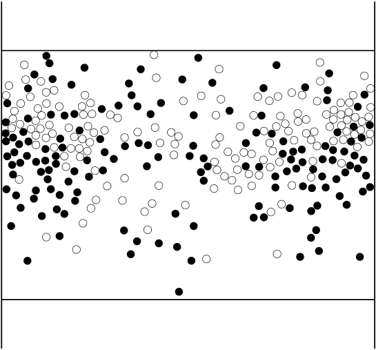
Figure 1: Typical snapshot of the system described in III. Open circles indicate particles of species 1, black circles particles of species 2.

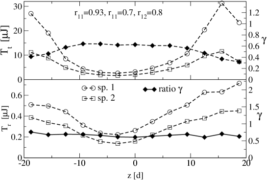
Figure 2: Top panel: Translational temperature profiles for species 1 (circles) and species 2 (squares) for a mass ratio $m_{2}/m_{1}=3.03$, expressed in $\mu J$ (left scale), and temperature ratio (diamonds) $T_{2}/T_{1}$ (right scale). The vertical position is measured in particle diameters ($d$) relative to the geometric center of the cell. Bottom panel: rotational temperature profiles for species 1 (circles) and species 2 (squares) and temperature ratio $T_{2}/T_{1}$ (diamonds).

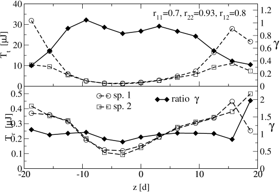
Figure 3: Same as in fig.1, but with different restitution coefficients.

III Results for a short system

The box dimensions were $L_{x}=48\,d$ and $L_{y}=32\,d$. Simulation runs were carried out using $N_{1}=150$ grains of each species. The static friction coefficient has been always chosen as $\mu=0.1$. The stationary state is determined by the balance between the energy input provided by the vibrating walls at a frequency of $50$ Hz and the dissipation due to inelastic collisions. The typical collision frequencies are of the order of $\nu_{1}\sim 580$ Hz and $\nu_{2}\sim 850$ Hz for the heavy and light balls, respectively. A typical microscopic configuration of the system is shown in fig.1.

III.1 Temperature profiles

The restitution coefficients were first set to $r_{11}=0.93$ for 1-1 collisions, $r_{22}=0.7$ for 2-2, and $r_{12}=0.8$ for 1-2 collisions. This means that the more massive particles are also the more elastic ones. In figure 2 we show the partial translational temperature profiles for the two species, and observe that close to the vertical boundaries the two temperatures are essentially determined by the energy injected by the vibrating walls. Indeed, interparticle collisions are rare within this region, and play no signifcant role because of the low local density (see figure 4). In addition, grains 1 and 2 impinging with the same speed on the mobile wall bounce with the same velocity ($V\propto A\omega$), hence the local value of the temperature ratio, $\gamma=T_{2}/T_{1}$ near the vibrating walls, turns out to be approximately $\gamma\sim m_{1}/m_{2}$, as shown in figure 2.

On the other hand, the temperature drops as the distance from the walls increases, while the ratio $\gamma$ grows up to a plateau value, indicating that collisions tend to cool the mixture and render the two partial temperatures closer. Figure 2 clearly displays the breakdown of the kinetic energy equipartition already noticed in previous experimental and theoretical studies.

We also measured the rotational temperature profiles, shown in figure 2. We observe for rotational temperatures the same kind of equipartition breakdown that holds for translational degrees of freedom. Moreover, the absolute values of rotational and translational temperatures are quite different, as already reported by Luding Luding for a one-component, vibrated granulate. On the other hand, the ratio of the two rotational temperature profiles seems to be quite close to that of the translational temperature profiles.

In figure 3, we changed the restitution coefficients and set $r_{11}=0.7$, $r_{22}=0.93$ for 2-2, and $r_{12}=0.81$. Therefore now the more massive particles are the more inelastic. We observe that, whereas the temperature profiles near the vibrating planes are nearly unchanged, because collisions are rare, the value of the temperature of the heavier species is lower and the temperature ratio is closer to $1$. In this case the larger inelasticity of the heavier particles competes with the mass asymmetry which instead tends to make $T_{2}/T_{1}$ smaller.

III.2 Area fraction profiles

Due to the large value of the parameter $\Gamma$, the partial density profiles tend to be rather symmetric, with a maximum near the center. We also notice small differences in the density profiles, which reveal that the heavier species has higher concentration close to the center of the cell, while the lighter species is more spread.

Comparing the present results for the area fraction profiles with those recently obtained by employing a Direct Simulation Monte Carlo technique Pagnani , we notice that the agreement is only qualitative, whereas the temperature ratios are in significantly better agreement.

We verified that removing tangential friction (coupling the translational and rotational degrees of freedom) does not change significantly the above scenario. In fact, the translational temperature and density profiles of the cases $\mu=0$ and $\mu=0.1$ show only small quantitative differences, more pronounced close to the horizontal walls.

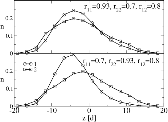
Figure 4: Area fraction profiles $n_{1}$ and $n_{2}$. Control parameters are the same as in fig. 1.

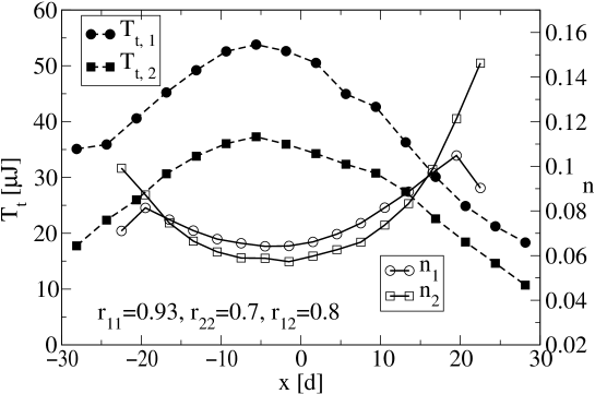
Figure 5: Temperature profiles $T_{1}$ e $T_{2}$ (left scale) along the horizontal direction and area fractions $n_{1}$ and $n_{2}$ (right scale). Control parameters are the same as in fig. 1.

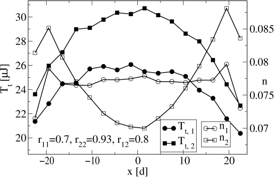
Figure 6: Same as in figure 5, but with different restitution coefficients.

III.3 Transversal profiles

We also studied the density and temperature profiles along the horizontal direction. To the best of out knowledge, no such measure has been reported in experimental works. In figures 5 and 6 we observe that temperature profiles vanish close to side walls, while density profiles display their maxima in the same region. In order to gain further insight, we analyzed a sequence of snaphsots of the dynamics, and observed that the system bears a denser cloud of grains in the vicinity of one of the side walls. Such a configuration was maintained over an interval of time much longer than the vibration period $2\pi/\omega$.

The cluster eventually “evaporates” to form again close to a randomly selected side wall. Over several periods of oscillation of the cell, we noticed an effective horizontal simmetry breaking, i.e. the number of particles in the right-hand and left-hand sides of the cell were rather different. The system is unstable with respect to horizontal density fluctuations and clusterizes spontaneously, until the vibrating bases wash out the cluster.

Moreover, we also observed some spontaneous tendency of the system to segregate the species, a fact which becomes more apparent at high densities. Both phenomena have their origin in the inelasticity. A possible qualitative explanation of the observed dynamics is as follows: particles with smaller restitution coefficient tend to group together, since the more energy they dissipate through 2-2 collisions, the denser the segregated domain becomes. Particles with higher restitution coefficient bounce for a longer time after a collision, and dilate more quickly.

III.4 Velocity Probability Distributions

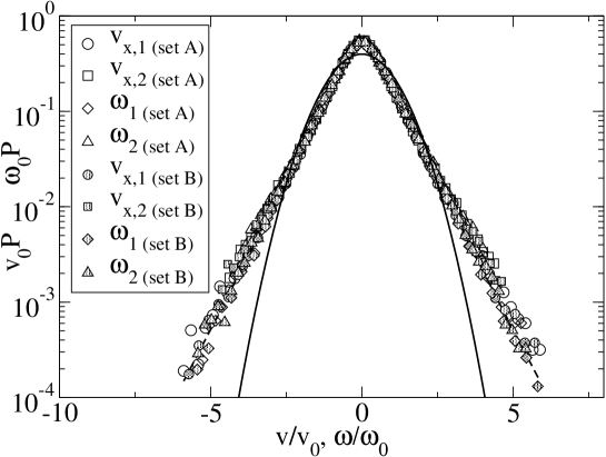
Figure 7: Rescaled velocity distribution functions $<c>P(c)=f(c/<c>)$ for translational velocities and angular velocities of both species. Set A corresponds to parameters of fig. 2, set B to parameters of fig. 3. The independent variables ($v$, $\omega$) were rescaled by their mean squared value ($v_{0}$, $\omega_{0}$). On rescaling, the distributions collapse nicely onto each other. The dashed curve is the fitting law discussed in the text, the continuous line is the Gaussian plotted as a reference for the eye.

Figure 7 shows the distributions functions for the translational velocities along the horizontal direction. For sake of comparison, all the velocities were rescaled by their mean square values. We notice that the two transversal velocity distribution functions deviate from a Gaussian and are fitted by $f(c)=A/(exp(\beta c^{\alpha})+exp(-\beta c^{\alpha}))$, with: $A=1.068$, $\beta=1.74$, $\alpha=0.918$ .

The exponential tails appear to have a smaller slope than the theoretically predicted 3/2 value, for a uniform system stochastically driven vannoije . We notice the phenomenon already reported in Pagnani : the rescaled velocity distribution of lighter species display higher tails.

Figure 7 also shows the angular velocity distributions (rescaled by their mean square value, see caption).

Our simulations show that such distributions have pronounced non-Gaussian tails. The angular velocity distributions can be described by the same scaling function we used for translational velocity distributions.

III.5 Collision time distribution

Recently Blair and Kudrolli utilizing high speed digital photography measured the collision statistics of grains bound to move on an inclined plane blair_poster . They determined the distribution of path lengths, $P(l)$ and showed that it deviates from the theoretical prediction for elastic hard spheres. In particular, $P(l)$ shows a peak in the small $l$ region, not present in elastic systems. In order to assess the existence of such a behavior in the IHS model we performed similar measurements. Figure 8 displays the results for the collision times of the two species. One clearly sees that the probability density that a particle suffers a collision in a short interval is enhanced with respect to the elastic case. The physical reason for that lies in the existence of strong correlations which lead to the presence of clusters where the path lengths are shorter than in a uniform system. For the sake of comparison we plotted in figure 8 also the corresponding distribution of an elastic gas having the same density and granular temperature of our inelastic mixture. The effect of the shorter average collision time is clearly visible. We also notice that the ratio of the collision frequencies is approximately equal to the the ratio of the average velocities, as expected from elementary kinetic arguments.

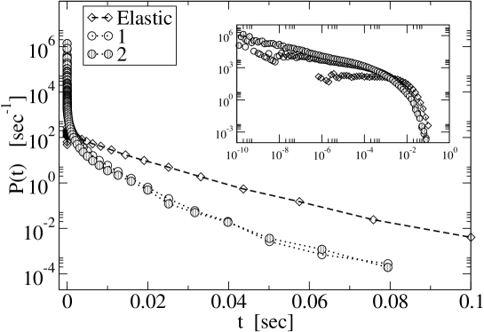
Figure 8: Probability distribution functions of the collision times for the two components (system with $r_{11}=0.93$, $r_{22}=0.7$, $r_{12}=0.8$). For comparison we plotted the corresponding distributions for an elastic system. The inset shows the same curves in bilogarithmic scale.

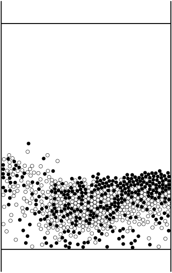
Figure 9: Snapshot of the system described in IV. Open circles indicate particles of species 1, black circles particles of species 2.

IV Long system

In the case of a box of dimensions $L_{x}=48\,d$ and $L_{y}=64\,d$ with $300$ grains of each species the effect of gravity is much more evident, resulting in a stronger inhomogeneity and asymmetry of the system. In fact, the density and temperatures profiles are not symmetric with respect to the vertical direction. A configuration of such system is shown in fig. 9. Most of the particles remain suspended above the bottom wall and are hit by those which are between the bottom wall and and the bulk. Very few particles reach the upper vibrating wall, so that the granular temperature of the system is much lower in the top than in the bottom. The partial temperature profiles and density profiles are shown in fig. 10. One sees that near the lower vibrating wall the temperature profiles are similar to those of the shorter system, whereas in the bulk they are appreciably different. The average ratio is lower than in the $L_{y}=32$ d case. An interesting feature present in fig.10 is the presence of a region of increasing temperatures. Such a phenomenon has been predicted by the hydrodynamic theory of Brey et al. Brey . The theory predicts a temperature varying as $T\sim z^{3/2}$ in the region above the minimum. Such a prediction is verified by our simulation results.

Physically, the increase is due to the competition between the energy input from the walls and the small dissipation due to the reduced number of collisions associated with the low density region. This can be appreciated in the inset of figure 10 where the quantity $\xi(z)=n(z)T(z)^{3/2}$ is shown: $\xi(z)$ is proportional to the energy dissipation due to inelastic collisions among particles, being the collision rate $\propto nT^{1/2}$ and the average dissipated energy in a single collision $\propto T$. The graph of $\xi(z)$ reveals that the energy dissipation is much more relevant in the bottom region than in the middle and upper regions.

Correspondingly the velocity PDF shows an interesting behavior (see figure 11). In fact, the shape of the rescaled PDF becomes narrower with the height. In the central region the measured PDF resembles the exponential PDF measured in the short system (figure 7), whereas in the bottom region the PDF has more extended tails. Such a lack of universality in the velocity PDf was noted experimentally by Blair and Kudrolli blair . It was also noticed in puglisi1 : there it was shown that the tails of the PDF became broader when the dissipation rate was increased. Here the mechanism is similar: the broader PDFs are those measured in the bottom region, where the dissipation rate is higher.

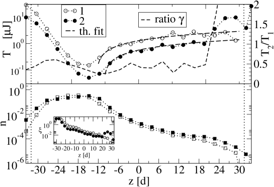
Figure 10: Temperature and area fraction profiles for the system discussed in section IV. In the inset the dissipation rate $\xi(z)$ is shown. In the figure we compared our result against the hydrodynamic prediction $T\sim z^{3/2}$ (solid lines). The vertical dotted lines correspond to the rest position of the horizontal boundaries.

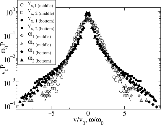
Figure 11: Rescaled velocity distribution functions for the $48\times 64$ system measured at different heights.

V Conclusion

Summarizing, we studied a systems of inelastic particles in vertically vibrated containers and subject to the gravitational field. The system was numerically investigated by using an Event-Driven dynamics, which affords the exploration of a wide range of dynamical parameters. We examined two similar setups which differ only for the aspect ratio of the container and for the number of particles.

In the shorter system we determined the partial granular temperatures, their ratio, and the area fraction profiles along the vertical direction. Those measures are in qualitative agreement with the experimental results, but a quantitative comparison requires a more detailed knowledge of the experimental parameters. Physically the lack of energy equipartition between the two species has two causes: a) the vibrating walls feed energy proportionally to the mass of each species; b) the dissipation is in general different for the two components. The two effects may conspire (for example if the heavier species is the more elastic) to give a small value of the temperature ratio or they may cancel and give a temperature ratio close to one (for example when the heavier species is the more inelastic). Moreover, we observed that density profiles are non-uniform along the horizontal direction, as well, indicating that the particles tend to clusterize in the vicinity of side walls. We also measured the velocity distributions, verifying that they can be collapsed onto each other, under proper rescaling, and the scaling function has a stretched exponential behavior. Finally the distribution of flight times between succesive collisions has been measured and compared to that of an elastic system: the inelasticity has the effect of enhancing the statistics of very short times.

In the longer system we have again obtained the temperature and area fraction profiles, observing a stronger inhomogeneity and asymmetry. In this case the area fraction is much larger near the bottom wall, reaching higher values than in the previous experiment. The middle-upper region seems to be qualitatively well described by recent hydrodynamic theories developed for one component systems. Here the velocity PDFs display a non-universal behavior, with broader tails in the more dense (and dissipative) regions.

VI Appendix

In order to make it simpler for the reader to interpret the present model, we present an appendix in which we explicitly state the collision rulesFarkas .

The colliding particles are characterized by radii $R_{1}$ and $R_{2}$, positions ${\bf r}_{1}$ and ${\bf r}_{2}$, translational velocities ${\bf v}_{1}$ and ${\bf v}_{2}$ and rotational (angular) velocities $\boldsymbol{\omega}_{1}$ and $\boldsymbol{\omega}_{2}$ (we assume that if $\boldsymbol{\omega}$ is parallel and in the direction of the $z$ axis, than the rotation is anticlockwise if seen from above the $xy$ plane). We introduce the normal unitary vector joining the centers of the particles ${\bf n}=({\bf r}_{2}-{\bf r}_{1})/|{\bf r}_{2}-{\bf r}_{1}|$ and the tangential unitary vector ${\bf t}$ obtained rotating ${\bf n}$ by an anti-clockwise angle $\pi/2$. Then we introduce the relative velocity ${\bf g}$, the velocity of the center of mass ${\bf V}$ and the velocities of the particles in the center of mass frame $\boldsymbol{\zeta}_{1}$ and $\boldsymbol{\zeta}_{2}$:

$${\bf g} ={\bf v}_{1}-{\bf v}_{2}$$ (2a)

$${\bf V} =\frac{m_{1}{\bf v}_{1}+m_{2}{\bf V}_{2}}{m_{1}+m2}$$ (2b)

$$\boldsymbol{\zeta}_{1} =\frac{m_{eff}}{m_{1}}{\bf g}$$ (2c)

$$\boldsymbol{\zeta}_{2} =-\frac{m_{eff}}{m_{2}}{\bf g}$$ (2d)

where $m_{eff}=m_{1}m_{2}/(m_{1}+m_{2})$.

Then we decompose the relative velocity ${\bf g}$ on the orthonormal basis given ${\bf n}$ and ${\bf t}$, as well as the velocities of the particles in the center of mass frame, i.e.:

$$g_{n} =({\bf v_{1}}-{\bf v_{2}})\cdot{\bf n}$$ (3a)

$$g_{t} =({\bf v_{1}}-{\bf v_{2}})\cdot{\bf t}$$ (3b)

$$\zeta_{n\beta} =\frac{m_{eff}}{m_{\beta}}g_{n}$$ (3c)

$$\zeta_{t\beta} =\frac{m_{eff}}{m_{\beta}}g_{t}$$ (3d)

with $\beta=1,2$ the index of the particle.

We finally introduce $g_{c}$ as the relative circular velocity at the point of contact and $g_{r}$ as the total tangential relative velocity (circular and translational) at the point of contact:

$$g_{c} =R_{1}\omega_{1}+R_{2}\omega_{2}$$ (4a)

$$g_{r} =g_{c}+g_{t}$$ (4b)

To characterize the collision rules we use a model that take into account a reduction of normal relative velocity ($g_{n}$), a reduction of total tangential relative velocity ($g_{r}$) and an exchange of energy between those two degrees of freedom. The reduction of normal relative velocity is modeled as usual by means of a restitution coefficient $\alpha\in[0,1]$:

$$g_{n}^{\prime}=-\alpha g_{n}.$$ (5)

We assume a dependence of $\alpha$ by the relative velocity of the form:

$$\alpha(g_{n})=\left\{\begin{array}[]{lll}1-(1-\alpha_{0})\frac{|g_{n}|}{v_{0}}^{\frac{3}{4}}&\mbox{ per }&g_{n}<v_{0}\\ \alpha_{0}&\mbox{ per }&g_{n}>v_{0}\end{array}\right.$$

where $\alpha_{0}$ is a constant which stands for $r_{ij}$, $v_{0}=\sqrt{gD}$, with $D$ the average diameter of the particles (and $g$ is the gravity acceleration). From equations (5) we obtain the update of normal velocities in the center of mass frame:

$$\zeta_{n1}^{\prime} =-\alpha\frac{m_{eff}}{m_{1}}g_{n}$$ (6a)

$$\zeta_{n2}^{\prime} =\alpha\frac{m_{eff}}{m_{2}}g_{n}$$

What lacks now is an expression for the tangential and angular velocities after the collisions. We distinguish between two possible cases: sliding or sticking collisions. The condition that allows to determine if a collision is sticking or sliding is the following:

$$\frac{|g_{r}|}{g_{n}}\geq\frac{l+1}{l}\mu(1+\alpha)$$ (7)

where $l$ is the adimensionalized inertia moment and is equal to $1/2$ or $2/5$ if the particle is a disk or a sphere respectively, while $\mu$ is the static friction coefficient of the surface of the particles which in the following will be assumed to be equal to the dynamic friction coefficient.

In the sliding case we use the following rules to update the tangential components of the velocities of the particles in the center of mass frame:

$$\zeta_{t1}^{\prime} =\zeta_{t1}-\mu(1+\alpha)\frac{m_{eff}}{m_{1}}g_{n}sign(g_{r})$$ (8a)

$$\zeta_{t2}^{\prime} =\zeta_{t2}+\mu(1+\alpha)\frac{m_{eff}}{m_{2}}g_{n}sign(g_{r})$$ (8b)

$$R_{1}\omega_{1}^{\prime} =R_{1}\omega_{1}-\frac{\mu(1+\alpha)}{l}\frac{m_{eff}}{m_{1}}g_{n}sign(g_{r})$$ (8c)

$$R_{2}\omega_{2}^{\prime} =R_{2}\omega_{2}-\frac{\mu(1+\alpha)}{l}\frac{m_{eff}}{m_{2}}g_{n}sign(g_{r})$$ (8d)

In the case of a sticking collision, instead, the update rules are obtained considering that:

$$\zeta_{t1}^{\prime}-\zeta_{t2}^{\prime}+R_{1}\omega_{1}^{\prime}+R_{2}\omega_{2}^{\prime}=0$$ (9)

from which, after calculations, one gets:

$$\zeta_{t1}^{\prime} =\frac{1}{l+1}\zeta_{t1}-\frac{l}{l+1}\frac{m_{eff}}{m_{1}}(R_{1}\omega_{1}+R_{2}\omega_{2})$$ (10a)

$$\zeta_{t2}^{\prime} =\frac{1}{l+1}\zeta_{t2}+\frac{l}{l+1}\frac{m_{eff}}{m_{2}}(R_{1}\omega_{1}+R_{2}\omega_{2})$$ (10b)

$$R_{1}\omega_{1}^{\prime} =R_{1}\omega 1\left[\frac{l}{l+1}+\frac{m_{eff}}{(l+1)m_{2}}\right]$$ (10c)

$$-R_{2}\omega_{2}\frac{m_{eff}}{(l+1)m_{1}}-\frac{1}{l+1}\zeta_{t1}$$ (10d)

$$R_{2}\omega_{2}^{\prime} =R_{2}\omega 2\left[\frac{l}{l+1}+\frac{m_{eff}}{(l+1)m_{1}}\right]$$ (10e)

$$-R_{1}\omega_{1}\frac{m_{eff}}{(l+1)m_{2}}+\frac{1}{l+1}\zeta_{t2}$$ (10f)

The velocity of particles in the absolute frame are finally obtained in the two cases (considering that the center of mass is not perturbed by the collision) by the equation:

$$\mathbf{v}^{\prime}_{\beta}=\mathbf{V}+\zeta_{n\beta}^{\prime}\mathbf{n}+\zeta_{t\beta}^{\prime}\mathbf{t}$$ (11)

(for particle of index $\beta$) leading to the following global collision rule for translational velocities:

$$\mathbf{v}_{1}^{\prime} =\mathbf{v}_{1}-(1+\alpha)\frac{m_{2}}{m_{1}+m_{2}}[(\mathbf{v}_{1}-\mathbf{v}_{2})\cdot\mathbf{n}]\mathbf{n}-\left\{\begin{array}[]{lll}sign(g_{r})\mu(1+\alpha)\frac{m_{2}}{m_{1}+m_{2}}[(\mathbf{v}_{1}-\mathbf{v}_{2})\cdot\mathbf{n}]\mathbf{t}\mbox{ (sliding)}\\ \frac{m_{1}-lm_{2}}{(l+1)(m_{1}+m_{2})}[(\mathbf{v}_{1}-\mathbf{v}_{2})\cdot\mathbf{t}]\mathbf{t}-\frac{l}{l+1}\frac{m_{2}}{m_{1}+m_{2}}(R_{1}\omega_{1}+R_{2}\omega_{2})\mbox{ (stick)}\end{array}\right.$$ (12c)

$$\mathbf{v}_{2}^{\prime} =\mathbf{v}_{2}+(1+\alpha)\frac{m_{1}}{m_{1}+m_{2}}[(\mathbf{v}_{1}-\mathbf{v}_{2})\cdot\mathbf{n}]\mathbf{n}+\left\{\begin{array}[]{lll}sign(g_{r})\mu(1+\alpha)\frac{m_{1}}{m_{1}+m_{2}}[(\mathbf{v}_{1}-\mathbf{v}_{2})\cdot\mathbf{n}]\mathbf{t}\mbox{ (sliding)}\\ \frac{m_{2}-lm_{1}}{(l+1)(m_{1}+m_{2})}[(\mathbf{v}_{1}-\mathbf{v}_{2})\cdot\mathbf{t}]\mathbf{t}+\frac{l}{l+1}\frac{m_{1}}{m_{1}+m_{2}}(R_{1}\omega_{1}+R_{2}\omega_{2})\mbox{ (stick)}\end{array}\right.$$ (12f)

while for rotational velocities:

$$R_{1}\omega_{1}^{\prime} =\left\{\begin{array}[]{lll}R_{1}\omega_{1}-\frac{\mu(1+\alpha)}{l}\frac{m_{2}}{m_{1}+m_{2}}g_{n}sign(g_{r})\mbox{ (stick)}\\ R_{1}\omega 1\left[\frac{l}{l+1}+\frac{m_{1}}{(l+1)(m_{1}+m_{2})}\right]-R_{2}\omega_{2}\frac{m_{2}}{(l+1)(m_{1}+m_{2})}-\frac{1}{l+1}\zeta_{t1}\mbox{ (slide)}\\ \end{array}\right.$$ (13c)

$$R_{2}\omega_{2}^{\prime} =\left\{\begin{array}[]{lll}R_{2}\omega_{2}-\frac{\mu(1+\alpha)}{l}\frac{m_{1}}{m_{1}+m_{2}}g_{n}sign(g_{r})\mbox{ (stick)}\\ R_{2}\omega_{2}\left[\frac{l}{l+1}+\frac{m_{2}}{(l+1)(m_{1}+m_{2})}\right]-R_{1}\omega_{1}\frac{m_{1}}{(l+1)(m_{1}+m_{2})}+\frac{1}{l+1}\zeta_{t1}\mbox{ (slide)}\\ \end{array}\right.$$ (13f)

- (1) H.M. Jaeger, S.R. Nagel and R.P. Behringer, Rev. Mod. Phys. 68, 1259 (1996).
- (2) I.Goldhirsch and G.Zanetti, Phys.Rev.Lett. 70, 1619 (1993).
- (3) J.J.Brey, M.J. Ruiz-Montero, F. Moreno, R. Garcia-Rojo, cond-mat/0201435
- (4) A. Baldassarri, U. Marini Bettolo Marconi and A. Puglisi, Phys.Rev. E 65, 051301 (2002).
- (5) K. Feitosa e N. Menon, 2002,Phys.Rev. Lett. 88, 198301 (2002).
- (6) R.D. Wildman and D.J. Parker, Phys.Rev. Lett. 88, 064301 (2002).
- (7) S.R. Dahl, C.M. Hrenya, V. Garzó e J. W. Dufty,2002, cond-mat/0205413.
- (8) Vicente Garzó e James Dufty, Phys. Rev. E, 60 5706 (1999).
- (9) U. Marini Bettolo Marconi and A. Puglisi, Phys.Rev. E 65, 051305 (2002).
- (10) U. Marini Bettolo Marconi and A. Puglisi, Phys. Rev. E 66, 011301 (2002).
- (11) Alain Barrat e Emmanuel Trizac, 2002, cond-mat/0202297.
- (12) A.Pagnani, U. Marini Bettolo Marconi, and A. Puglisi, (cond-mat/0205619).
- (13) A. Barrat e E. Trizac, 2002, cond-mat/0207267.
- (14) O.R. Walton, Particulate Two-Phase Flow, M.C. Roco editor, Butterworth-Heinemann, Boston (1993), page 884.
- (15) C. Bizon, M. D. Shattuck, J. B. Swift and H. Swinney, Phys. Rev. E 60, 4340 (1999)
- (16) C. Cattuto, submitted to Computers in Science and Engineering.
- (17) A. Puglisi, V. Loreto, U. Marini Bettolo Marconi, A. Petri and A. Vulpiani, 1998 Phys. Rev. Lett. 81, 3848 and Phys. Rev. E 59, 5582 (1999).
- (18) S. McNamara and S.Luding, Phys.Rev. E 58, 2247 (1998).
- (19) A. Baldassarri, U. Marini Bettolo Marconi, A. Puglisi, A. Vulpiani Phys. Rev. E 64, 011301 (2001).
- (20) T. P. C. van Noije and M. H. Ernst, Granular Matter 1, 57 (1998).
- (21) D.L. Blair and A. Kudrolli, private comunication.
- (22) D.L. Blair and A. Kudrolli, Phys. Rev. E 64, 050301 (2001).
- (23) Z. Farkas, P. Tegzes, A. Vukics, T. Vicsek, cond-mat/9905094 version 7/5/1999.