Semiclassical approach to calculating the influence of local lattice fluctuations on electronic properties of metals

Abstract

We propose a new semiclassical approach based on the dynamical mean field theory to treat the interactions of electrons with local lattice fluctuations. In this approach the classical (static) phonon modes are treated exactly whereas the quantum (dynamical) modes are expanded to second order and give rise to an effective semiclassical potential. We determine the limits of validity of the approximation, and demonstrate its usefulness by calculating the temperature dependent resistivity in the Fermi liquid to polaron crossover regime (leading to ‘saturation behavior’) and also isotope effects on electronic properties including the spectral function, resistivity, and optical conductivity, problems beyond the scope of conventional diagrammatic perturbation theories.

]

I Introduction

The present-day understanding of electron-lattice interactions in metals is based on the assumption that typical phonon frequencies $\Omega$ are small relative to typical electron energies $t$, so that electronic properties may be calculated as an expansion in the adiabatic parameter $\gamma=\Omega/t$. This was first exploited by Migdal and Eliashberg (ME)[1] to derive a self-consistent set of equations for electron and phonon self-energies. Since ME theory neglects order $\gamma$ vertex corrections it wrongly predicts a zero result for most isotope effects on electronic properties (notable exceptions being the superconducting [2] and charge-ordering[3] transition temperatures). Furthermore, ME theory assumes that the underlying electronic groundstate can be described by Fermi liquid theory. However, if the electron-lattice coupling strength $\lambda=\Lambda/t$ exceeds a critical value (of order 1) the conduction electrons are believed to form “small polarons”,[4] so that the electronic groundstate is fundamentally reconstructed. In this case, although an expansion in $\gamma$ exists, the starting point is not clear.

Signatures of polaronic behavior have been observed in certain complex narrow band materials. Well-known examples are phonon mediated superconductors with high transition temperatures, like $\rm BiO$ based superconductors,[5] alkali-doped $\rm C_{60}$ fullerides,[6] and the A15 compounds,[7] and ‘colossal magnetoresistance’ (CMR) manganites.[8] Despite much work many questions remain open: as examples we cite a possible ‘saturation’ of the resistivity at high temperatures,[7] unexpected midinfrared transitions in the optical conductivity,[5, 6, 8] and large isotope effects on electronic properties. For instance, the CMR manganite $\rm(La_{0.25}Pr_{0.75})_{0.7}Ca_{0.3}MnO_{3}$ undergoes a metal-insulator transition upon $\rm{}^{16}O$ - $\rm{}^{18}O$ isotope substitution.[9] A calculational technique which can address with these issues is urgently needed.

The interaction of conduction electrons with local lattice fluctuations may be described by the dynamical mean field theory (DMFT).[10] In this approximation the electron self energy is momentum independent. Since the full frequency dependence is retained the corresponding one-electron Green function shows both coherent and incoherent features. Recent applications of DMFT to the electron-phonon problem include a systematic expansion in powers of $\gamma$,[11] several weak-coupling expansion schemes,[3, 12, 13] and a “classical” ($\gamma=0$) study of the Fermi liquid to polaron crossover. (Treating the $\gamma=0$ limit without assuming DMFT has not been possible yet.[15]) The expansion of Ref. [11] is restricted to very low temperatures and cannot access the intermediate or strong coupling regimes where important physics such as resistivity saturation or polaronic effects is expected. Because of the mismatch between phonon and electron energy scales numerical simulations[12] are difficult to implement accurately, except in the “antiadiabatic” limit $\gamma\sim 1$ of unclear physical relevance.

Here we propose a new “semiclassical” method for treating intermediate and strong couplings in the physically relevant limit $\gamma\ll 1$. We treat the classical (static) phonon modes exactly (as in Ref.[14]) and expand the quantum (dynamical) modes to second order. The resulting action consists of a classical part plus an effective semiclassical potential. The method is valid for a wide range of electron-phonon couplings and resulting groundstates. Here we consider only electron-phonon interactions (i.e. the Holstein model). However, the method can be generalized (along the lines of Ref.[11, 16]) to study phonon effects in the presence of strong electron-electron interactions. We focus on the crossover regime between Fermi liquid and polaron physics which was not easily tractable by previous methods. The remainder of the paper is organized as follows. In Sec. II we introduce the Holstein model and the semiclassical method. In Sec. III we discuss additional simplifications which are convenient for numerically implementing the method. Sec. IV studies analytical limits and defines the observables (spectral function, resistivity and optical conductivity) we consider. Numerical results are presented and discussed in Sec. V. We conclude in Sec. VI.

II Model and Formalism

In this paper we study the Holstein model[17] of electrons interacting with local lattice fluctuations: $H_{\rm hol}=H_{\rm el}+H_{\rm ph}+H_{\rm el-ph}$ with

$$H_{\rm el} = -\sum_{ij}t_{i-j}\,c^{\dagger}_{i\sigma}c^{\phantom{\dagger}}_{j\sigma}-\mu\sum_{i}\left(c^{\dagger}_{i\sigma}c^{\phantom{\dagger}}_{i\sigma}-n\right)\;,$$ (1)

$$H_{\rm ph} = \frac{1}{2\Lambda}\sum_{i}\left(r^{\,2}_{i}+\dot{r}^{2}/\Omega^{2}\right)\;,$$ (2)

$$H_{\rm el-ph} = \sum_{i}r_{i}\left(c^{\dagger}_{i\sigma}c^{\phantom{\dagger}}_{i\sigma}-n\right),$$ (3)

where we have absorbed the electron phonon coupling into the phonon coordinate $r$ which thus has dimension of energy as does the phonon stiffness parameter $\Lambda$. In our numerical calculations we further specialize to a mean electron density per spin direction of $n=1/2$ (this implies $\mu=0$) and we use the semicircular density of states $\rho(\epsilon)=(1/N)\,\sum_{\vec{k}}\delta(\epsilon-\epsilon_{\vec{k}})=1/(2\pi t^{2})\sqrt{4t^{2}-\epsilon^{2}}$ (per spin), where $\epsilon_{\vec{k}}$ is the Fourier transform of $t_{i-j}$. However, our approach is not restricted to these cases. The possibility of charge-density wave formation (due to a nested Fermi surface) will not be considered in this work, but could also be considered via our method.

The fundamental assumption of DMFT is the momentum independence of the electron self energy $\Sigma(\vec{p},i\,\omega_{n})\rightarrow\Sigma_{n}\equiv\Sigma(i\,\omega_{n})$. This implies that the physics can be derived from an impurity model specified by the action

$$S(\{r_{k}\};\{c_{n}\}) = (T/2\Lambda)\,\sum_{k}r_{k}\,\left(1+\omega_{k}^{2}/\Omega^{2}\right)\,r_{k}^{*}\,-n\,r_{0}$$ (5)

$$-(2s+1)\,{\rm Tr\,\,ln}\left[c_{n}\,\delta_{nm}-T\,r_{n-m}\right]\;.$$

The $c_{n}$ are mean field functions which describe the conduction electrons and depend on odd Matsubara frequencies $\omega_{n}=2\pi T\,(n+1/2)$. The $r_{k}$ are bosonic fields which describe the phonons and depend on even Matsubara frequencies $\omega_{k}=2\pi T\,k$. The factor $(2s+1)$ is the spin degeneracy. The partition function may be written as a functional integral over the bosonic fields

$$Z=\int{\cal D}[r]\exp(-S).$$ (6)

It is a functional of the mean field function $c$. The impurity Green function ${\cal G}$ and self energy $\Sigma$ are defined by

$${\cal G}_{n}\equiv\frac{1}{2s+1}\,\frac{\delta\,\ln Z}{\delta\,c_{n}}\equiv\frac{1}{c_{n}-\Sigma_{n}(\{c_{n}\})}\;.$$ (7)

The mean field function is fixed by equating the local Green function ($G_{\rm loc}^{\rm lattice}(\omega)=\int\,\frac{d^{d}k}{(2\pi)^{d}}\,\frac{1}{\omega-\epsilon_{k}-\Sigma(\omega)}$) of the original lattice model to ${\cal G}_{n}$. For a semicircular density of states one finds[10]

$$c_{n}=i\omega_{n}+\mu-t^{2}\,{\cal G}_{n}\left(\{c_{n}\}\right)\;.$$ (8)

The effective action (5) defines an interacting quantum field theory which cannot be solved exactly. Here we expand the action to quadratic order in the quantum modes $\omega_{k}$ ($k\neq 0$) while treating the classical modes $\omega_{0}$ exactly:

$${\rm Tr\,\,ln}\left[c_{n}\,\delta_{nm}-T\,r_{n-m}\right]\approx{\rm Tr\,\,ln}\left[c_{n}\ -T\,r_{0}\right]-$$ (10)

$$\frac{T^{2}}{2}\sum_{n\neq m}(c_{n}-T\,r_{0})^{-1}\,r_{n-m}\,(c_{m}-T\,r_{0})^{-1}\,r_{m-n}\;.$$

The effective action $S=S_{0}+\sum_{k>0}S_{k}$ separates into a classical part $S_{0}$ and quadratic quantum parts $S_{k>0}$, both of which depend on $r_{0}$:

$$S_{0} = \frac{T}{2\Lambda}\,r_{0}^{2}-n\,r_{0}-(2s+1)\,{\rm Tr\,\,ln}\left[c_{n}\ -T\,r_{0}\right]$$ (11)

$$S_{k>0} = \frac{T}{\Lambda\Omega^{2}}\,r_{k}\,\left[\omega_{k}^{2}+\Omega_{k}^{2}(r_{0})\right]\,r_{k}^{*},$$ (12)

where

$$\Omega_{k}^{2}(r_{0})=\Omega^{2}\left[1+\Pi_{k}(r_{0})\right]$$ (13)

and

$$\Pi_{k}(r_{0})=(2s+1)\,\Lambda\,T\,\sum_{n}\frac{1}{c_{n}-T\,r_{0}}\,\frac{1}{c_{n-k}-T\,r_{0}}\;.$$ (14)

Since the dynamic action (12) is quadratic the $k\neq 0$ modes can be integrated out exactly. The resulting partition function

$$Z=\int{\rm d}r\,P(r)$$ (15)

may be written as a one-dimensional integral over the rescaled classical coordinate $r=T\,r_{0}$ and

$$P(r)=\exp\left\{-S_{0}(r)-\sum_{k>0}\ln\left[1+\frac{\Omega_{k}^{2}(r)}{\omega_{k}^{2}}\right]\right\}$$ (16)

is the (unnormalized) probability that the classical coordinate takes the value $r$. Note that $P(r)$ depends on the mean field parameters $c_{n}$ which must be computed self-consistently. Performing the derivative with respect to $c_{n}$ yields the local Green function

$${\cal G}_{n}=\frac{1}{Z}\,\int\,{\rm d}r\,P(r)\,\left[\frac{1}{c_{n}-r}+F_{n}(r)\,\left(\frac{1}{c_{n}-r}\right)^{2}\right]\;.$$ (17)

The function $F_{n}$ is given by

$$F_{n}(r)=\Lambda\,T\,\sum_{k>0}\,\frac{\Omega^{2}}{w_{k}^{2}+\Omega_{k}^{2}(r)}\,\left(\frac{1}{c_{n-k}-r}+\frac{1}{c_{n+k}-r}\right)\;.$$ (18)

Eqs. (8) and (17) form a complete set of equations which, in principle, can be solved for the local Green function on the imaginary Matsubara axis. However, the direct numerical implementation is difficult, especially if the local Green function is required for real frequencies. In the following section we discuss physical approximations which considerably simplify the numerical task and allow for analytical insights.

III Numerical implementation

A Static approximation

The rapid increase of $S_{k>0}$ as the phonon frequency $\omega_{k}$ is increased above the Debye frequency $\Omega$, combined with the observation that $\Pi_{k}$ varies with frequency on the scale $t$, means that when computing the $c_{n}$ [via Eq. (8)] as well as static and energetic quantities we may replace $\Pi_{k}(r_{0})$ by its zero frequency limit $\Pi_{0}(r_{0})$. (For a more formal justification see Refs.[1, 11].) Then $S_{k}$ is the action of a harmonic oscillator with renormalized frequency $\Omega(r)\equiv\Omega_{0}(r)=\Omega[1+\Pi(r,\omega=0)]^{1/2}$, and the phonon distribution function reads

$$P_{\rm static}(r)=\frac{\Omega(r)/2T}{\sinh\left(\Omega(r)/2T\right)}\,\exp\left(-S_{0}(r)\right)\;.$$ (19)

The function $F$ introduced above is given by

$$F_{n}(r)=\frac{\Lambda}{2}\,\frac{\Omega^{2}}{\Omega(r)}\,\frac{1}{c_{n}-r}\left[\coth\left(\frac{\Omega(r)}{2T}\right)-\frac{2T}{\Omega(r)}\right]\;.$$ (20)

in the static approximation. Note that $F_{n}\sim 1/T$ as $T\rightarrow\infty$. The form (20) is used in the iteration of the DMFT equation (8) on the Matsubara axis. We use up to 512 positive Matsubara frequencies and treat high frequencies analytically. At the end of this first DMFT cycle we obtain the phonon distribution function $P(r)$.

The scheme is stable (the ‘$k\neq 0$’ integration exists and $P(r)>0$) provided $\Omega^{2}(r)>-4\pi^{2}T^{2}$, in other words for all real renormalized phonon frequencies and a (temperature-dependent) range of imaginary ones. Note that $\Omega^{2}(r)$ increases as $|r|$ is increased from zero. An imaginary phonon frequency corresponds to an instability of the ground state, but if $T>|\Omega|/2\pi$ in this formalism thermal fluctuations re-stabilize the ground state. For imaginary $\Omega(r)$ one must analytically continue Eqs. (19), (20) to

$$P_{\rm static}(r)=\frac{|\Omega(r)|/2T}{\sin\left(|\Omega(r)|/2T\right)}\,\exp\left(-S_{0}(r)\right)$$ (21)

and

$$F_{n}(r)=\frac{\Lambda}{2}\,\frac{\Omega^{2}}{\left|\Omega(r)\right|}\,\frac{1}{c_{n}-r}\left[\frac{2T}{\left|\Omega(r)\right|}-\cot\left(\frac{\left|\Omega(r)\right|}{2T}\right)\right]\;,$$ (22)

respectively. The form (21) has to be used for low $T$, large $\Lambda$, and small $r$ (for example, the case $\Lambda=2.25$, $\Omega=0.1$, and $T<0.2$ [see below]).

As will be discussed in more detail below an imaginary renormalized phonon frequency is a precursor of polaronic effects. When the temperature is lowered we have $|\Omega(r)|/2T\rightarrow\pi$. If we introduce a small deviation $\epsilon(r)$ (increasing with $r$) via $|\Omega(r)|/2T=\pi-\epsilon(r)$ the semiclassical phonon distribution

$$P_{\rm static}(r)=\frac{\pi}{\epsilon(r)}\,\exp\left(-S_{0}\right)$$ (23)

is enhanced around $r\approx 0$ in the polaronic phase. This may be interpreted as a precursor effect of a “polaronic band” where quantum oscillations allow for nearest neighbor polaron tunneling. An analysis of the regime $T<|\Omega(r)|/2\pi$ requires a different treatment not given here.

B Dynamic corrections

For dynamical quantities, like the optical conductivity, frequency corrections to $\Pi_{0}$ will be important at low temperatures (they lead e.g. to finite electron lifetimes) and the static approximation is not sufficient. Employing the full expression (18) in the calculation of the local Green function is cumbersome. To obtain ${\cal G}$ on the real frequency axis a numerically challenging continuation from the imaginary frequency axis has to be performed. We thus prefer to do all our calculations on the real axis. We begin by expanding

$$\Omega_{k}^{2}(r)=\Omega_{0}^{2}(r)+\left.\frac{{\rm\partial}\Omega_{k}^{2}(r)}{{\rm\partial}\omega_{k}}\right|_{k=0}\,\omega_{k}+{\cal O}(\omega_{k}^{2})\;.$$ (24)

On the real frequency axis this corresponds to an expansion in small frequencies which dominate dynamic quantities at low temperatures. The second term in Eq. (24) is imaginary and leads to a damping of the phonon modes and to small (relative order $\gamma$) corrections to physical results. We will neglect this feedback of the electrons on the phonon system and keep only the frequency renormalization, i.e. the first term in Eq. (24). This leads to

$$P(r)=P_{\rm static}(r)$$ (25)

and

$$F_{n}(r)=\Lambda\,T\,\sum_{k>0}\,\frac{\Omega^{2}}{w_{k}^{2}+\Omega^{2}(r)}\,\left(\frac{1}{c_{n-k}-r}+\frac{1}{c_{n+k}-r}\right)\;.$$ (26)

Note the difference to the static approximation [Eq. (20)] where the finite frequency transfer of $\omega_{k}$ in the effective electron fields $c_{n-k}$ and $c_{n+k}$ is missing. Eq. (26) defines the correct $F$ for calculating dynamic quantities from $P_{\rm static}(r)$. In the following we will restrict ourselves to the regime of stable quantum modes where $P_{\rm static}(r)$ is well defined down to $T=0$. It is easy to analytically continue the function $F$ to the real axis. The real and imaginary parts read

$$F^{{}^{\prime}}(\omega,r)=\frac{\Lambda}{2}\,\frac{\Omega^{2}}{\Omega_{r}}\times$$ (30)

$$\left[\;b(\Omega_{r})\,{\cal P}^{{}^{\prime}}(\omega+\Omega_{r})-b(-\Omega_{r})\,{\cal P}^{{}^{\prime}}(\omega-\Omega_{r})-\right.$$

$$\;\;\;(2T/\Omega_{r})\,{\cal P}^{{}^{\prime}}(\omega)+$$

$$\left.\;\;\;\frac{1}{\pi}\,{\rm P}\int\,{\rm d}\epsilon\,{\cal P}^{{}^{\prime\prime}}(\epsilon)\,f(\epsilon)\,\left(\frac{1}{\omega-\Omega_{r}-\epsilon}-\frac{1}{\omega+\Omega_{r}-\epsilon}\right)\right]$$

and

$$F^{{}^{\prime\prime}}(\omega,r)=\frac{\Lambda}{2}\,\frac{\Omega^{2}}{\Omega_{r}}\times$$ (34)

$$\left[\;b(\Omega_{r})\,{\cal P}^{{}^{\prime\prime}}(\omega+\Omega_{r})-b(-\Omega_{r})\,{\cal P}^{{}^{\prime\prime}}(\omega-\Omega_{r})-\right.$$

$$\;\;\;(2T/\Omega_{r})\,{\cal P}^{{}^{\prime\prime}}(\omega)-$$

$$\left.\;\;\;f(\omega-\Omega_{r})\,{\cal P}^{{}^{\prime\prime}}(\omega-\Omega_{r})+f(\omega+\Omega_{r})\,{\cal P}^{{}^{\prime\prime}}(\omega+\Omega_{r})\right]$$

Here $f(\omega)$ and $b(\omega)$ are the Fermi and Bose distributions, respectively. ${\cal P}^{{}^{\prime}}$ and ${\cal P}^{{}^{\prime\prime}}$ denote the real and imaginary part of ${\cal P}(\omega+i0^{+})\equiv 1/[c(\omega)-r]$, respectively, $\Omega_{r}\equiv\Omega(r)$ and the integral in Eq. (30) is a principal value. If the propagators ${\cal P}$ exhibit particle-hole symmetry then $F^{{}^{\prime}}(\omega)=-F^{{}^{\prime}}(-\omega)$ and $F^{{}^{\prime\prime}}(\omega)=F^{{}^{\prime\prime}}(-\omega)$. The real part is an odd function of frequency and the modifications arising from a finite $\Omega_{r}$ may be ignored at $\omega\approx 0$. To leading order in $\Omega_{r}$ we are left with

$$F(\omega,r)=\frac{\Lambda}{2}\,\frac{\Omega^{2}}{\Omega_{r}}\,[b(\Omega_{r})\,{\cal P}(\omega)-b(-\Omega_{r})\,{\cal P}(\omega)+$$ (36)

$$i\,f(\omega+\Omega_{r})\,{\cal P}^{{}^{\prime\prime}}(\omega)-i\,f(\omega-\Omega_{r})\,{\cal P}^{{}^{\prime\prime}}(\omega)-(2T/\Omega_{r})\,{\cal P}(\omega)]\;.$$

Dynamic corrections reduce the imaginary part of $F$ at small frequencies. For $T=0$ and $r=0$ the static approximation yields a non-zero value $F^{{}^{\prime\prime}}\sim\gamma$ for small $\omega$ whereas including finite frequency corrections give $F^{{}^{\prime\prime}}_{T=0}=0$ in a shell $-\Omega_{0}<\omega<\Omega_{0}$.

The results of this section constitute an expansion in $\gamma$, and have errors of order $\gamma^{2}$. However, for temperatures smaller then the renormalized phonon frequency the (quantum modified) thermal fluctuations become of order $\gamma^{2}$ and one of the order $\gamma^{2}$ errors induced by the semiclassical approach leads on the real axis to a self energy whose imaginary part changes sign, so the self energy becomes non-causal [see below Eq. (49)]. We thus suggest two complementary ad hoc schemes for iterating the DMFT equations on the real frequency axis. Both schemes result in a causal electron self-energy and ${\cal O}(\gamma^{2})$ or ${\cal O}(\gamma T)$ corrections to physical quantities.

(i) Setting $F(\omega,r)\equiv 0$ for all $\omega$ and $r$. This approach gives the correct high temperature behavior and is also a good approximation for $T=0$, and we expect it to give us an idea how the high and low temperature regimes of dynamic quantities are connected. Furthermore, the imaginary part of $F$ does indeed vanish for small enough frequencies at zero temperature—as we would expect on physical grounds since the resistivity should drop to zero in a Fermi liquid state.

(ii) The violation of causality is only of order $\gamma^{2}$, as we will show in the next section. In order to obtain a well-defined electron self energy we may therefore add a heuristic impurity scattering rate $\tau\sim\gamma$ to the self energy:

$${\cal G}\longrightarrow\left({\cal G}^{-1}+i\,\tau\right)^{-1}$$ (37)

We discuss a proper choice of $\tau$ in the next section.

Note that when crossing over from the Fermi liquid to the polaronic regime the renormalized frequency $\Omega(r=0)$ tends to zero. We believe that for $\lambda=\lambda_{c}$ the ‘$F=0$’ approach (which is then practically identical to the classical case) becomes exact for properties which involve only electrons at the Fermi energy. This would imply a square root like resistivity $\rho\sim T^{1/2}$ down to $T=0$ at this singular point.[14] For coupling constants slightly below $\lambda_{c}$ the suggested approaches (i) and (ii) should give a reasonable picture down to lowest temperatures.

To summarize, the effect of quantum phonons to order $\gamma$ is to add a semiclassical potential to the classical action. Static and energetic quantities, including the distribution function of onsite lattice distortions $r$, may be calculated using a simplified (‘static’) semiclassical potential depending only on a renormalized frequency $\Omega(r)$. The approach is valid for all coupling strengths $\lambda$ but is restricted to temperatures $T>|\Omega(r=0)|/2\pi$ in the polaronic regime $\lambda>\lambda_{c}\approx 2.2$ where $\Omega(r)$ becomes imaginary. Some additional numerical effort (compared to the classical case[14]) is required due to the calculation of the renormalized frequencies. Care has to be taken when calculating dynamical quantities at low temperatures due to the presence of an additional quantum scattering term. We propose two schemes for incorporating dynamic corrections on top of the simplified semiclassical action. For coupling strengths $\lambda<\lambda_{c}$, i.e. in the Fermi liquid regime, the crossover between the high and low temperature behavior of transport properties can be studied.

IV Discussion and Observables

A Fermi liquid to polaron crossover

When discussing the influence of local lattice fluctuations on electronic properties one has to distinguish between two regimes. For small values of $\Lambda$ the conduction electrons are weakly renormalized quasiparticles. This is the Fermi liquid regime. For large $\Lambda$ the conduction electrons are self-trapped by their own local lattice distortions. This is the polaronic regime. In the classical case[14] ($\gamma=0$) the main features of the “polaronic transition” may be illustrated by expanding to quadratic order around $r=0$:

$$S_{0}=\frac{1}{2\,\Lambda\,T}\left(1+\Lambda\,\Gamma_{2}\right)\,r^{2}$$ (38)

with

$$\Gamma_{\alpha}=(2s+1)\,T\,\sum_{n}\,c_{n}^{-\alpha}\;.$$ (39)

For later use we define

$$\bar{\Lambda}_{\rm classical}=\frac{\Lambda}{1+\Lambda\,\Gamma_{2}},\;\;\;\;\bar{\Omega}_{\rm classical}=\Omega\,\sqrt{1+\Lambda\,\Gamma_{2}}\;.$$ (40)

As long as $\Lambda<-1/\Gamma_{2}\equiv\Lambda_{c}^{\rm classical}$, $S_{0}$ is minimized by $r=0$. In the $T\rightarrow 0$ limit the dominant contributions to $Z$ come from small distortions. If $\Lambda$ approaches $\Lambda_{c}^{\rm classical}$ from below, the elastic energy vanishes and the system enters a polaronic state with $\langle r\rangle\neq 0$. The critical $\Lambda_{c}$ depends on band filling, temperature, $\Lambda$, $\Omega$, as well as other parameters (such as electron-electron interaction strength). In the noninteracting case [where $c^{0}_{n}=\frac{i}{2}\,[\omega_{n}+\sqrt{\omega_{n}^{2}+4t^{2}}]$ (upper half plane)] and at $T=0$ we find $\Lambda_{c}=3\pi t/[(2s+1)\,4]$. It has been shown[14] that at high temperatures electrons are strongly affected by the presence of a local (polaronic) lattice instability. A strongly coupled system turns from a Fermi liquid into a polaronic insulator with activated conduction caused by the hopping of small polarons. In the crossover regime the system can be characterized as a “bad metal”. This intermediate state is the focus of the current paper.

We now discuss the changes to this picture introduced by quantum effects. We first focus on the regime of stable quantum modes, i.e. $\Lambda<\Lambda_{c}$. For small lattice distortions we may expand the effective phonon frequency around $r=0$. At half filling we find

$$\Omega^{2}(r)=\Omega^{2}\,\left(1+\Lambda\,\Gamma_{2}+3\,\Lambda\Gamma_{4}\,r^{2}\right)\;.$$ (41)

In the regime under consideration we can assume $1+\Lambda\,\Gamma_{2}>0$ and use Eq. (19) to calculate the effective partition function. To second order in $r$ and at low temperatures the semiclassical action reads

$$S=\frac{1}{2\,\Lambda\,T}\times$$ (44)

$$\left[\Lambda\,\Omega\,\sqrt{1+\Lambda\,\Gamma_{2}}+\left(1+\Lambda\,\Gamma_{2}+\frac{3}{2}\,\frac{\Lambda^{2}\,\Omega}{\sqrt{1+\Lambda\,\Gamma_{2}}}\,\Gamma_{4}\right)\,r^{2}\right]$$

$$\equiv S(r=0)+\frac{1}{2\,\bar{\Lambda}\,T}\,r^{2}\;.$$

The first ($r=0$) term is the Migdal correction to the classical action given in Eq. (38). It arises from the one-phonon-loop diagrams.[11] Quadratic and higher orders in the distortions have to be considered at higher temperatures or stronger couplings, especially if the system is close to the instability $\Lambda_{c}$. In terms of the dimensionless parameters

$$\lambda=\Lambda/t\,,\;\;\;\gamma=\Omega/t\,,$$ (45)

the leading corrections to the classical action are of the form $\bar{\lambda}^{n}_{\rm classical}\,\bar{\gamma}_{\rm classical}$ with $n\geq 2$, i.e. they are of order $\bar{\gamma}_{\rm classical}$. Notice however that the corrections can become arbitrary large if $\Lambda\rightarrow\Lambda_{c}^{\rm classic}$.[19]

The $T=0$ polaronic instability occurs when the coefficient of $r^{2}$ in Eq. (44) vanishes, i.e. when (in rescaled units)

$$1+\lambda_{c}\,(t\Gamma_{2})+\frac{\lambda_{c}^{2}\,\gamma\,3(t^{3}\Gamma_{4})/2}{\sqrt{1+\lambda_{c}\,(t\Gamma_{2})}}=0\;.$$ (46)

This equation has a solution at $\lambda_{c}=\lambda_{c}(\gamma)=-\Gamma_{2}/t+{\cal O}(\gamma^{2/3})$. Because $\Gamma_{4}>0$ (for the Holstein model at half filling $\Gamma_{4}=(2s+1)\,8/(15\,\pi\,t^{3})$ in the noninteracting limit) we see that quantum fluctuations increase the critical coupling needed for the polaronic instability by an amount $\delta\lambda\sim\gamma^{2/3}$. Note also that the sign of $\bar{\Omega}^{2}_{\rm classical}=\Omega^{2}(r=0)$ is only determined by $\Gamma_{2}$. The system enters the regime of unstable quantum modes at coupling strength $\lambda\approx\lambda_{c}^{\rm classic}<\lambda_{c}(\gamma)$. As we shall see, this leads to an interesting precursor effect of polaronic behavior.

B Low-temperature self energy

In this section we discuss the low temperature self energy in detail, in order to clarify the limitations of our theory. For weak to intermediate coupling strengths, $\Lambda<\Lambda_{c}$, $P(r)$ is peaked about $r=0$ with half-width of order $T$, so an expansion in $r$ is justified if $\bar{\lambda}\,T/t\ll 1$, i.e. if $T$ is low and the system is not too close to the polaronic instability. It is convenient to rewrite Eq. (17) to order ${\cal O}(\bar{\lambda}_{\rm classical}^{2}\,\bar{\gamma}_{\rm classical}^{2},\bar{\lambda}_{\rm classical}^{2}\,T^{2}/t^{2})$ by adding and subtracting the $k=0$ term in $F_{n}$ and moving all terms to the denominator, so (denoting $\frac{1}{Z}\,\int\,{\rm d}r\,P(r)$ by $\langle\,\rangle$)

$${\cal G}_{n}=\left\langle\frac{1}{c_{n}-r-\Sigma_{n}^{\rm Migdal}(r)-\bar{\Lambda}_{\rm classical}(r)\,T/(c_{n}-r)}\right\rangle$$ (47)

with

$$\Sigma_{n}^{\rm Migdal}(r)=\Lambda\,T\sum_{k=-\infty}^{k=\infty}\frac{\Omega^{2}}{\omega_{k}^{2}+\Omega_{k}^{2}(r)}\,\frac{1}{c_{n-k}-r}\;.$$ (48)

At low $T$ and not too close to the polaronic instability we may proceed by expanding ${\cal G}$ to order $r^{2}$, averaging, and then replacing terms in the denominator. This leads to a self energy

$$\Sigma_{n}^{\rm lowT}=\Sigma_{n}^{\rm Migdal}(r=0)+\bar{\gamma}_{\rm classical}\,T\,A_{n}\;.$$ (49)

The expression for $A_{n}$ is somewhat cumbersome, because many terms contribute and the result depends on the relative values of external and phonon frequency. However, in all cases we have examed, the analytic continuation of $A_{n}\rightarrow A(\omega+i0^{+})$ has an imaginary part of positive sign, corresponding to a non-causal contribution to $\Sigma$, and magnitude of order unity ($\bar{\gamma}^{0}$). For example, if one assumes that all relevant contributions in the occuring Matsubara sums stem from small frequencies $|\omega_{n\pm k}|<<2t$ then (noting $c_{n}=i\,t\,{\rm sgn}\,\omega_{n}$ at half filling)

$$A(\omega=0) = i\,\frac{\bar{\lambda}_{\rm classical}-\bar{\lambda}}{\bar{\gamma}_{\rm classical}}+i\,\bar{\lambda}_{\rm classic}\,\bar{\lambda}$$ (50)

$$= i\,\left[\frac{3}{2}\,\bar{\Lambda}^{3}_{\rm classic}\,\Gamma_{4}+\bar{\lambda}_{\rm classic}\,\bar{\lambda}\right]\;.$$ (51)

The non-causal self energy is of order ${\cal O}(\bar{\gamma}_{\rm classical}\,T)$, i.e. formally ${\cal O}(\bar{\gamma}^{2}_{\rm classical})$, and is seen from the derivation to arise from an incomplete treatment of the ${\cal O}(\gamma^{2})$ contributions to physical quantities. Unfortunately at $(\omega,T)\ll\Omega$, the leading contribution $\Sigma_{\rm Migdal}\sim\Omega\,s(\Omega/T)$ where $s\sim\exp[-\Omega/T]$ as $T\rightarrow 0$, so the non-causal correction term dominates.

This may be viewed in a different way: a purely classical approximation ($\Omega\rightarrow 0$) would lead to a $T$-linear scattering rate with coefficient of order unity. The semiclassical approximation overcorrects for this behavior, cancelling the leading term leaving a correction of order $\gamma T$ but of the wrong sign.

The unphysical low temperature behavior is not due to the realization of the semiclassical approach introduced in Eq. (26). Starting from the full expressions Eqs. (17) and (18) we find a similar result

$$\bar{\Lambda}_{\rm classic}-\bar{\Lambda}\approx\bar{\Lambda}^{2}_{\rm classic}\,\Lambda\,2(2s+1)\,T^{2}\times$$ (53)

$$\sum_{n}\,\sum_{k>0}\frac{\Omega^{2}}{\omega_{k}^{2}+\Omega_{k}^{2}}\,\left[\frac{1}{c^{3}_{n}}\left(\frac{1}{c_{n+k}}+\frac{1}{c_{n-k}}\right)+\frac{1}{c_{n}^{2}}\frac{1}{c_{n+k}^{2}}\right]$$

which will also lead to a non-causal self energy. We conclude, that higher orders of quantum contributions $\gamma^{n}$ are required to completely suppress the thermal contributions at low temperatures $T<\bar{\Omega}$ (which wrongly would lead to a linear resistivity in $T$).

However, the thermal fluctuations are reduced in the semiclassical approach compared to the classical ($\gamma=0$) case by a factor $\gamma$ and the low-temperature self-energy is of order $\bar{\gamma}^{2}_{\rm classic}$, as can be seen from Eqs. (49) and (50):

$$\Sigma^{{}^{\prime\prime}}(\omega=0)=\frac{\bar{\Omega}^{2}_{\rm classic}}{t}\,f\left(\frac{T}{\bar{\Omega}_{\rm classic}}\right)\;,$$ (54)

where $f$ is a scaling function. Therefore, an order $\bar{\gamma}_{\rm classic}$ impurity scattering rate $\tau$, as proposed in the previous section, will lead to a well-defined electron self-energy. An appropriate choice may be found from Eq. (20). In the classical limit ($\bar{\Omega}_{\rm classic}\rightarrow 0$) we find

$$F_{n}(r=0)=\frac{\Lambda}{12}\,\frac{\Omega^{2}}{T}\,c_{n}^{-1},$$ (55)

i.e. a scattering rate $\tau\approx\bar{\lambda}_{\rm classical}\,\bar{\Omega}_{\rm classical}/12$ for temperatures $T\leq\bar{\Omega}_{\rm classical}$. This is the value we choose for the additional impurity contribution. Note that in the quantum limit ($T\rightarrow 0$) the static approach gives $\tau\approx\bar{\lambda}_{\rm classical}\,\bar{\Omega}_{\rm classical}/2$.

C Observables

We end this section by introducing the four observables we have investigated numerically: phonon distribution function, electron spectral function, optical conductivity, and resistivity. The normalized phonon distribution function $p(r)=P(r)/Z$ was defined above. Within DMFT the spectral function and optical conductivity can be derived from the electron self-energy on the real frequency axis. The density of states is given by

$$\rho(\omega)=\int{\rm d}\epsilon\,\rho_{0}(\epsilon)\,\rho(\epsilon,\omega)$$ (56)

with the spectral function defined by

$$\rho\left(\epsilon_{\vec{k}},\omega\right)=-\frac{1}{\pi}\,{\rm Im}\left[\frac{1}{\omega+\mu-\Sigma(\omega)-\epsilon_{\vec{k}}}\right]\;.$$ (57)

The optical conductivity is obtained from linear response theory applied to the expectation value of the current operator

$$j=\sum_{p}\left(\frac{{\rm\partial}\epsilon_{p}}{{\rm\partial}p}\right)\,c_{p}^{\dagger}c_{p}$$ (58)

In performing the sums over momentum $p$ we will assume a hypercubic lattice.[18] The differences to a Bethe lattice are not significant for the results presented here. The locality of the electron self energy implies that the momentum summation can be performed independently on each side of an electron-phonon vertex when calculating the expectation value of the current. Since the electron velocity $\partial\epsilon_{p}/\partial p$ is an odd function of momentum all vertex corrections vanish and the optical conductivity is obtained by a convolution of two full Green functions:

$$\sigma(\Omega)=\sigma_{0}\times$$ (60)

$$\int{\rm d}\omega\,\left(-\frac{f(\omega+\Omega)-f(\omega)}{\Omega}\right)\,\int{\rm d}\epsilon\,\rho_{0}(\epsilon)\,\rho(\epsilon,\omega)\,\rho(\epsilon,\omega+\Omega)$$

where $\sigma_{0}$ is a constant and $f(\omega)$ is the Fermi distribution. The resistivity of the system can be deduced from the optical conductivity via $\rho_{\rm DC}=1/\sigma(0)$. We briefly discuss $\rho_{\rm DC}$ in the regime $\Lambda<\Lambda_{c}^{\rm classic}$ where the quantum modes are stable. If $\Sigma^{{}^{\prime\prime}}(\omega=0)\ll 2t$ as $T\rightarrow 0$, the low temperature DC conductivity is given by

$$\sigma(0)=\frac{\pi}{2}\,\sigma_{0}\,\rho(0)\,\int\,\frac{{\rm d}\omega}{2T}\,\frac{1}{\cosh^{2}(\omega/2T)}\,\frac{1}{|\Sigma^{{}^{\prime\prime}}(\omega,T)|}$$ (61)

and we expect (for a Fermi liquid ground state) $\rho_{\rm DC}\sim{\rm const}+T^{2}$. However, due to the low-temperature defect of the semiclassical approach discussed above this regime cannot be reached.

V Results

In this section we apply the semiclassical method developed above to a system of spinless electrons ($s=0$) interacting with local lattice distortions, which is relevant to half-metals such as CMR manganites. First we consider high to intermediate temperatures. As discussed in section III.B the high to low temperature crossover of dynamical quantities can be discussed within the ‘$F=0$’ implementation of the semiclassical approach. This will be done first. A detailed comparison with other approaches will be given below, when discussing the low temperature behavior.

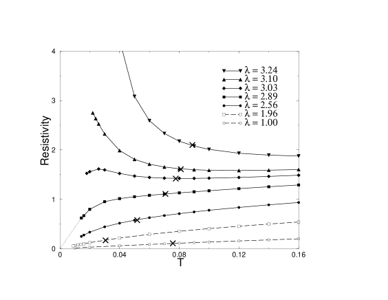
FIG. 1.: Resistivity as a function of temperature $T$ for various electron-phonon coupling strengths $\lambda$ at a given phonon frequency $\gamma=0.1$. Temperatures corresponding to the renormalized phonon frequency $|\Omega(r=0)|$ (taken at $T=0.2$) are indicated by a cross for each value of $\lambda$. Dashed and solid lines correspond to the regime of stable ($\lambda<\lambda_{c}^{\rm class}$) and unstable ($\lambda>\lambda_{c}^{\rm class}$) quantum modes, respectively. The low $T$ behavior in the regime of unstable quantum modes is beyond the scope of this paper and the dotted line for $\lambda=2.89$ serves as guide to the eye.

Fig. 1 shows the resistivity as a function of temperature for a wide range of coupling strengths and $\gamma=0.1$. For narrow electron bands (typical for e.g. the A-15 materials) this choice corresponds to setting $\Omega\sim 300$K. At high temperatures $T\gg\Omega$ we reproduce the results of the classical ($\gamma=0$) approach.[14, 20] At weak couplings the resistivity depends linearly on temperature $\rho(T)=AT+B$. At intermediate couplings the resistivity becomes nonlinear in $T$ and the ratio $A/B$ decreases. As discussed in detail in Ref. [20] this is essential for the phenomenon of ‘resistivity saturation’ in models which couple local lattice vibrations to the level positions: the scattering rate of the electrons with lattice fluctuations increases with $T$, but less rapidly than predicted from second order perturbation theory. Notice that when discussing resistivity saturation we focus on temperatures above the (renormalized) Debye temperature indicated by a cross in Fig. 1. As seen in Fig. 1 the system remains metallic for coupling strengths well above $\lambda_{c}^{\rm classic}=2.36$ because quantum lattice fluctuations allow the electrons to tunnel between neighboring sites. The crossover to the high temperature resistivity (which is large) is more pronounced than for a conventional metal. We thus refer to this state as a bad metal. Our approach is capable of describing this interesting state where quantum (Migdal) and thermal (classical) fluctuations compete. The strong renormalization of the phonon frequencies leads to a drop in resitivity at a temperature which depends strongly on $\lambda$ and which is well below the unrenormalized Debye temperature $\Omega=0.1$. Only for stronger couplings $\lambda>3.03$ does the resistivity show insulating behavior over the entire accessible temperature range.

FIG. 2.: Resistivity as a function of temperature $T$ for intermediate electron-phonon coupling strength $\lambda=2.89>\lambda_{c}^{\rm class}=2.36$ and various phonon frequencies. Quantum fluctuations destroy the polaronic insulator and restore a metallic state.

The new feature brought by quantum fluctuations to these curves is a coexistence of very weak temperature dependence at high $T$ with metallic behavior at low $T$. This is clearly shown in Fig. 2, which displays the effect of changing quantum fluctuations on the $\lambda=2.89$ curve of Fig. 1. One sees that the nearly classical model ($\gamma=0.01$) is an insulator at low $T$, while the other two are metals, while the higher-$T$ behavior is hardly affected. The $\gamma=0.1$ data bear a striking resemblance to the resistivity of well known saturation materials such as $\rm Nb_{3}Sb$.[7] We also note that the data shown in Fig. 2 imply an isotope-driven metal insulator transition, although to obtain this coupling one must finetune $\lambda$ within ${\cal O}(\gamma)$ of the critical value.

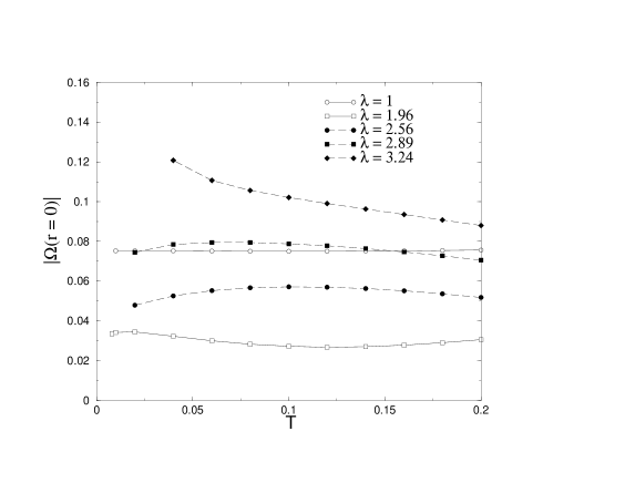
FIG. 3.: Renormalized phonon frequency $|\Omega(r=0)|$ as function of temperature $T$ for various coupling strengths $\lambda$ at a given phonon frequency $\gamma=0.1$. Close to the (classic) polaronic instability a clear temperature dependence is visible. For $\lambda=1.96$ the relative change of $|\Omega(r=0)|$ amounts to $12\%$ over the plotted temperature regime. Solid and dashed lines indicate the regime of stable [real $\Omega(r=0)$] or unstable [imaginary $\Omega(r=0)$] quantum modes, respectively.

In Fig. 1 we indicated the modulus of the renormalized phonon frequency by a cross. However, $|\Omega(r=0)|$ may be considerably temperature dependent. Fig. 3 shows the temperature dependence of the renormalized phonon frequency $|\Omega(r=0)|$. For weak couplings (e.g. $\lambda=1$) the frequency is slightly suppressed and nearly independent of temperature. However, close to the (classic) polaronic instability $\lambda_{c}^{\rm classic}$ (e.g. $\lambda=1.96$) the phonon frequency is strongly renormalized towards zero and temperature dependent. Nonmonotonic temperature dependence of phonon frequencies was found in models with interactions between phonons and strongly correlated electrons and was used to interpret anomalies in Raman scattering and acoustic experiments on certain superconducting molecular crystals.[21] Here we show that even pure electron-phonon coupling may lead to a nonmonotonic temperature dependence of the phonon frequency. Note, however, that the connection between $|\Omega(r=0)|$ and measurable quantities remains yet to be established. On entering the regime of unstable quantum modes the temperature dependence of the renormalized phonon frequency change qualitatively. In addition, an enhancement of the phonon frequency is possible. In the insulating regime $|\Omega(r=0)|(T)$ increases monotonically.

FIG. 4.: LOWER PANEL: Distribution of local distortions $P_{\rm static}(r)$ for three different phonon frequencies and $T=0.2$ (dotted lines), $T=0.1$ (dashed lines), and $T=0.04$ (solid lines). The coupling strength equals $\lambda=2.89$. Scales on $x$- and $y$-axes are the same in all plots and given in the first one. UPPER PANEL: Electron spectral function as function of frequency. The parameter values are identical to those in the lower panel. Scales on $x$- and $y$-axes are the same in all plots and given in the first one.

The collapse of the polaronic state due to quantum fluctuations causes other changes in electronic properties which are summarized in Figs. 4 and 5. The lower panel of Fig. 4 shows the distribution of local lattice distortions for various frequencies and the uppper one the spectral function. Fig. 5 displays the optical conductivity. At high temperatures we find a considerable probability for finite (dynamic) lattice distortions even in the metallic state. The density of states at the Fermi energy is relatively small and the Drude peak in the optical conductivity is very broad. In fact, the optical spectral weight can be spread over a frequency range which continously increase with increasing temperature. Therefore the term “saturation” is a misnomer: There is no intrinsic maximum value of the high-temperature resistivity.[20, 22]. Upon lowering the temperature we recover a conventional metallic state, where the probability of strong lattice distortions decreases, the density of states at the Fermi energy increases, and the Drude peak sharpens.

FIG. 5.: Optical conductivity $\sigma(\omega)$ for three different phonon frequencies and $T=0.2$ (dotted lines), $T=0.1$ (dashed lines) and $T=0.04$ (solid lines). The coupling strength equals $\lambda=2.89$. Scales on $x$- and $y$-axes are the same in all plots and given in the first one.

In a polaronic insulator there are pronounced negative (positive) distortions indicating that the electrons (holes) remain on a given site for a sufficiently long time for the lattice to relax. If the phonon frequency increases the probability at $r\approx 0$ becomes larger, which points to an increased electron mobility. As a consequence, three maxima in $P_{\rm static}(r)$ may be observed when crossing over from high to low temperatures for sufficiently large phonon frequency. The upper panel of Fig. 4 shows the corresponding changes in the spectral function of the electrons. The polaronic insulator exhibits a (pseudo) gap. The ‘splitting’ of the band is caused by dynamical local distortions. Upon increasing $\gamma$ one sees that at low $T$ considerable spectral weight is transferred from high to low energies, filling up the gap, whereas the spectral function at high $T$ is virtually unchanged. Further insight may be obtained by considering the optical conductivity (Fig. 5). For $\gamma=0.01$ we see an insulating gap develop from a broad, incoherent high-$T$ conductivity; again increasing the phonon frequency leads to the development of a low $T$ metallic state.

FIG. 6.: Resistivity as a function of temperature $T$ for $\lambda=1.96$, $\gamma=0.1$, calculated using various implementations of the semiclassical approach: (i) Static approximation $\Pi_{k}\rightarrow\Pi_{0}$ (static, dotted line), (ii) expansion in $\omega_{k}$ (dynamic, dashed line), (iii) neglecting $F$ (solid line, left panel) and (iv) adding an impurity scattering (solid line, right panel). For details see text and section III. The deficiencies of approaches (i) (nonmonotonic resisitivity) and (ii) (negative resisitivity, i.e. non-causal self energy) are clearly visible.

The technical difficulties mentioned in the previous section limited the calculation shown in Fig. 4 and 5 to relatively high temperatures. We now turn to the low-temperature behavior ($T<\Omega$) to reveal the strengths and weakness of different low-$T$ implementations of the semiclassical approach. We focus on $(\lambda,\gamma)=(1.96,0.1)$. Fig. 6 shows the low-temperature resistivity, calculated using various implementations of the semiclassical approach. Quantum lattice fluctuations enter in two places: the distribution function of lattice distortions $P(r)$ and the generalized contribution $F_{n}(r)$ to the electron self energy. The two properties influence the resistivity in opposite ways. A higher probability of small distortions decreases the resistivity whereas a negative $F^{\prime\prime}(\omega,r)$ describes additional electron-lattice scattering.

The implementations discussed here only differ in the choice of $F$ as discussed in section III.B. The static approximation gives $F_{n}(r=0)=(\bar{\Lambda}_{\rm classic}\,\bar{\Omega}_{\rm classic}/2)\,c_{n}^{-1}-\bar{\Lambda}_{\rm classic}\,T\,c_{n}^{-1}$ at very low temperatures and leads to a nonmonotonic resistivity, as seen in Fig. 6 (dotted line). When we take into account that $F$ has to be reduced for energies around the Fermi energy, the finite resistivity at zero temperature of the static approximation is eliminated but the resulting electron self energy now violates causality. Fig. 6 shows that the resistivity drops to zero at a finite temperature (dashed line). We conclude that at very low temperatures dynamic corrections of higher orders (see section III.B) become important. To mimic their effect we suggested, first, to set $F\equiv 0$. This is good at high to intermediate temperatures but cannot account for a Fermi liquid like resisitivity, $\rho_{\rm DC}\sim{\rm const}+T^{2}$ as seen in the left panel of Fig. 6 (solid line). Second, we suggested adding an impurity scattering of order $\gamma$ to obtain a well defined electron self energy. This is shown in the right panel of Fig. 6 (solid line): at very low temperatures the resistivity levels off to a finite value due to the added impurity scattering. Both (‘$F=0$’ and impurity) approaches demonstrate the development of a resistivity $\rho\sim T^{1/2}$ at $\lambda=\lambda_{c}^{\rm classical}$ and $T\rightarrow 0$.

FIG. 7.: MAIN PANEL: Density of states as function of frequency near the Fermi energy for $(\lambda,\gamma)$ = $(1.96,0.1)$ and various temperatures. The polaronic feature which appears at $\omega\approx 0$ is responsible for the strong decrease of the resistivity. INSET: Imaginary part of the generalized contribution of the quantum lattice fluctuations to the electron self energy $F(\omega,r)$ as function of frequency $\omega$ at zero distortion $r=0$ (parameter as in the main panel and $T=0.02$). Energy conservation reduce the scattering in a shell around the Fermi energy.

The inclusion of impurity scattering is an ad hoc remedy. However, it can be used to demonstrate the formation of polaronic bands. In the calculation leading to the spectral function in Fig. 4 we neglected the generalized contributions of the quantum lattice fluctuations to the electron self energy completely, i.e. $F\equiv 0$. In a bad metal, as seen in Fig. 4, this leads to an increase of spectral weight in a broad energy range around the Fermi energy when the temperature is lowered. However, $F$ should be frequency dependent. Additional scattering of electrons with quantum lattice fluctuations is possible for electrons sufficiently far from the Fermi energy as enforced by energy conservation (absorption and emission of finite frequency phonons). The frequency dependence of the scattering rate is illustrated in the inset of Fig. 7 which displays the imaginary part of $F(\omega,r=0)$ as given in Eq. (36). Even the sign changes near $\omega=0$ which compensates partially scattering from thermal fluctuations. This physics is captured by the impurity approach and leads to a clearly visible polaronic band in the spectral function as seen in the main panel of Fig. 7. For weak to intermediate coupling strengths, $\Lambda<\Lambda_{c}^{\rm classic}$, the phonon distribution function $P_{\rm static}(r)$ is concentrated around $r\approx 0$. Therefore, at $T=0$ the electron self energy is given by the Migdal expression, see Eq. (49), and a similar polaronic peak in the spectral function like here at finite temperatures can be observed at zero temperature.[23] However, the three peak structure of $P(r)$ as seen in Fig. 4 developing close to $\Lambda_{c}(\gamma)$ is clearly beyond the Migdal approach.

VI Conclusion

In this paper we have developed a semiclassical approach based on the dynamical mean field theory to treat the interactions of electrons with local dynamic lattice distortions. The method is not restricted to small or strong electron-phonon couplings. It can be applied to three spatial dimensions and may be extended to include interactions other than electron-phonon. The effective action is organized in terms of local static $n$-point correlation functions $\Gamma_{n}$ which have to be appropriately modified in the presence of other interactions. However, the frequency dependence of $\Gamma_{n}$ cannot be neglected alltogether. At low temperatures it leads to additional electron-lattice scattering which is important when calculating dynamical quantities. We discussed the effect of these dynamic corrections extensively. Nevertheless, errors of order $\gamma^{2}$ inherent in the semiclassical approach allow only for a qualitative discussion of the low temperature behavior by introducing an impurity scattering of order $\gamma$ by hand. A quantitative analysis is beyond the scope of this paper and left for future work. However, at a critical coupling $\lambda=\lambda_{c}^{\rm classic}=3\pi/[(2s+1)4]$ a classical picture should hold and the resistivity becomes $\rho\sim T^{1/2}$ for very low temperatures.

We have applied our method to study isotope effects on electronic properties in the crossover regime between Fermi liquid and polaronic behavior. We found large effects including an isotope-driven insulator-to-metal transition. The phenomena described in Sec. V may be relevant for various half-metals such as CMR manganites and A15 compounds even though the simplicity of the model studied here does not allow for detailed comparisons with experiments. Nevertheless, an isotope-driven insulator-to-metal transition was observed[9] in $\rm(La_{0.25}Pr_{0.75})_{0.7}Ca_{0.3}MnO_{3}$. Within the picture proposed above this can be understood as a quantum tunneling effect. In addition to electron-phonon interactions, a realistic description of conduction electrons in the CMR manganites must account for double exchange with the core spins of the Mn ions. This would amplify the insulator-to-metal transition observed above: if the electrons become mobile the core spins tend to order ferromagnetically in order to further lower the electron kinetic energy.

We have also addressed the question of resistivity saturation in metals with high resistivity. Quantum lattice fluctuations shift the polaronic instability to larger couplings $\delta\lambda\sim\gamma^{2/3}$. Therefore, systems with strong quantum lattice fluctuations remain metallic up to larger electron-phonon couplings than systems with purely classical (thermal) fluctuations which implies a stronger violation of the validity of second order perturbation theory. We may (misleadingly) speak of resistivity saturation although there is no upper bound for the high-temperature resistivity in contrast to models which couple atomic vibrations to electron hopping matrix elements.[22] The resistivity at high temperatures assumes very large values and a pronounced change in slope of the temperature dependent resitivity is obtained when crossing over from high to low temperatures. The smoothness of the crossover can be changed by isotope replacements without changing the strength of the electron-phonon coupling.

Acknowledgements SB thanks M. Calandra and G. Zwicknagl for useful discussions. SB acknowledges the DFG, the Rutgers University Center for Materials Theory and NSF DMR0081075 for financial support at early stages of this work; AD and AJM acknowledge NSF DMR0081075.

REFERENCES

- [1] A.B. Migdal, Sov. Phys. JETP 7, 996 (1958); G.M. Eliashberg, Sov. Phys. JETP 11, 696 (1960)
- [2] W.L. McMillan, Phys. Rev. 167, 331 (1968)
- [3] S. Blawid and A.J. Millis, Phys. Rev. B 63, 115114 (2001)
- [4] A.S. Alexandrov, V.V. Kabanov and D.K. Ray, Phys. Rev. B 49, 9915 (1994)
- [5] A.V. Puchkov et al, Phys. Rev. B 54, 6686 (1996)
- [6] L. Degiorgi et al, Phys. Rev. B 49, 7012 (1994)
- [7] Z. Fisk and G.W. Webb, Phys. Rev. Lett. 36, 1084 (1976)
- [8] Y. Okimoto and Y. Tokura, J. Supercond. 13, 271 (2000)
- [9] L.M. Belova, J. Supercond. 13, 305 (2000)
- [10] A. Georges, G. Kotliar, W. Krauth and M.J. Rozenberg, Rev. Mod. Phys. 68, 13 (1996)
- [11] A. Deppeler and A.J. Millis, Phys. Rev. B 65, 100301 (2002)
- [12] J.K. Freericks, M. Jarrell, D.J. Scalapino, Phys. Rev. B 48, 6302 (1993); J.K. Freericks and M. Jarell, Phys. Rev. B 50, 6939 (1994); J.K. Freericks, V. Zlatić, W. Chung and M. Jarrell, Phys. Rev. B 58, 11613 (1998)
- [13] S. Ciuchi and F. de Pasquale, Phys. Rev. B 59, 5431 (1999)
- [14] A.J. Millis, R. Mueller and B.I. Shraiman, Phys. Rev. B 54, 5389 (1996)
- [15] V.V. Kabanov and O.Y. Mashtakov, Phys. Rev. B 47, 6060 (1993)
- [16] A. Deppeler and A.J. Millis, cond-mat/0204617
- [17] T. Holstein, Ann. Phys. 8, 325 (1959); 8, 343 (1959)
- [18] T. Pruschke, M. Jarell and J.K. Freericks, Adv. Phys. 44, 187 (1995)
- [19] A. Deppeler and A.J. Millis, Phys. Rev. B 65, 224301 (2002)
- [20] A.J. Millis, J. Hu and S. Das Sarma, Phys. Rev. Lett. 82, 2354 (1999)
- [21] J. Merino and R.H. McKenzie, Phys. Rev. B 62, 16442 (2000)
- [22] M. Calandra and O. Gunnarsson, Phys. Rev. Lett. 87, 266601-1 (2001)
- [23] J.P. Hague and N. d’Ambrumenil, cond-mat/0106355