Effective resistivity of magnetic multilayers
A. Crépieux* and P. Bruno
Max-Planck-Institut für Mikrostrukturphysik, Weinberg
2, 06120 Halle, Germany
Abstract
In heterogeneous system, the correspondence between calculated
and measured quantities, such as the conductivity or the
resistivity, is not obvious since the former ones are local
quantities whereas the latter ones are often average values over
the sample. In this report, we show explicitly how the
correspondence can be done in the case of magnetic multilayers.
In the linear response regime, the electric current 𝐉 𝐉 {\bf J} 𝐫 𝐫 {\bf r} 𝐄 𝐄 {\bf E} 𝐫 ′ superscript 𝐫 ′ {\bf r}^{\prime} [1 ]
J i ( 𝐫 ) = ∫ − ∞ + ∞ 𝑑 𝐫 ′ ∑ j σ i j ( 𝐫 , 𝐫 ′ ) E j ( 𝐫 ′ ) , subscript 𝐽 𝑖 𝐫 superscript subscript differential-d superscript 𝐫 ′ subscript 𝑗 subscript 𝜎 𝑖 𝑗 𝐫 superscript 𝐫 ′ subscript 𝐸 𝑗 superscript 𝐫 ′ \displaystyle J_{i}({\bf r})=\int_{-\infty}^{+\infty}d{\bf r}^{\prime}\sum_{j}\sigma_{ij}({\bf r},{\bf r}^{\prime})E_{j}({\bf r}^{\prime}), (1)
where i 𝑖 i j 𝑗 j { x , y , z } 𝑥 𝑦 𝑧 \{x,y,z\} σ i j subscript 𝜎 𝑖 𝑗 \sigma_{ij} 𝐫 𝐫 {\bf r} 𝐫 ′ superscript 𝐫 ′ {\bf r}^{\prime} [2 ] as a current-current
correlation function
σ i j ( 𝐫 , 𝐫 ′ ) = lim ω → 0 1 ω ∫ 0 + ∞ 𝑑 t e i ω t ⟨ [ 𝐣 ( 𝐫 , t ) ; 𝐣 ( 𝐫 ′ , 0 ) ] ⟩ , subscript 𝜎 𝑖 𝑗 𝐫 superscript 𝐫 ′ subscript → 𝜔 0 1 𝜔 superscript subscript 0 differential-d 𝑡 superscript 𝑒 𝑖 𝜔 𝑡 delimited-⟨⟩ 𝐣 𝐫 𝑡 𝐣 superscript 𝐫 ′ 0
\displaystyle\sigma_{ij}({\bf r},{\bf r}^{\prime})=\lim_{\omega\rightarrow 0}\frac{1}{\omega}\int_{0}^{+\infty}dt\;e^{i\omega t}\left\langle\;\left[\;{\bf j}({\bf r},t)\;;\;{\bf j}({\bf r}^{\prime},0)\;\right]\;\right\rangle, (2)
where 𝐣 𝐣 {\bf j} [ A ; B ] = A B − B A 𝐴 𝐵
𝐴 𝐵 𝐵 𝐴 [\;A\;;\;B\;]=AB-BA ⟨ ⋯ ⟩ delimited-⟨⟩ ⋯ \langle\cdot\cdot\cdot\rangle 2 μ 𝜇 \mu
Let us start with a three-dimensional homogeneous system in the stationary regime. In this
case, the electric current and electric field do not dependent of
the position, thus Eq. (1 J i = ∑ j σ ¯ i j E j subscript 𝐽 𝑖 subscript 𝑗 subscript ¯ 𝜎 𝑖 𝑗 subscript 𝐸 𝑗 J_{i}=\sum_{j}\bar{\sigma}_{ij}E_{j}
σ ¯ i j ≡ ∫ − ∞ + ∞ 𝑑 𝐫 ′ σ i j ( 𝐫 , 𝐫 ′ ) , subscript ¯ 𝜎 𝑖 𝑗 superscript subscript differential-d superscript 𝐫 ′ subscript 𝜎 𝑖 𝑗 𝐫 superscript 𝐫 ′ \displaystyle\bar{\sigma}_{ij}\equiv\int_{-\infty}^{+\infty}d{\bf r}^{\prime}\;\sigma_{ij}({\bf r},{\bf r}^{\prime}), (3)
which is nothing else than the average value over the sample. The
𝐫 𝐫 {\bf r} 3 σ i j ( 𝐫 , 𝐫 ′ ) subscript 𝜎 𝑖 𝑗 𝐫 superscript 𝐫 ′ \sigma_{ij}({\bf r},{\bf r}^{\prime}) σ ¯ i j subscript ¯ 𝜎 𝑖 𝑗 \bar{\sigma}_{ij}
It is not more the case for heterogeneous systems because the
electric current and electric field are not uniform through the
sample. In this report, we treat the case of a multilayer formed
by a superposition of identical cells which have the dimension
{ a 0 , a 0 , L a 0 } subscript 𝑎 0 subscript 𝑎 0 𝐿 subscript 𝑎 0 \{a_{0},a_{0},La_{0}\} a 0 subscript 𝑎 0 a_{0} L 𝐿 L 𝐫 𝐫 {\bf r} 𝐑 𝐑 {\bf R} l 𝑙 l l 𝑙 l 1 1 1 L 𝐿 L 1
J i l 1 ( 𝐑 ) = ∫ − ∞ + ∞ 𝑑 𝐑 ′ ∑ j , l 2 σ i j l 1 l 2 ( 𝐑 , 𝐑 ′ ) E j l 2 ( 𝐑 ′ ) , superscript subscript 𝐽 𝑖 subscript 𝑙 1 𝐑 superscript subscript differential-d superscript 𝐑 ′ subscript 𝑗 subscript 𝑙 2
superscript subscript 𝜎 𝑖 𝑗 subscript 𝑙 1 subscript 𝑙 2 𝐑 superscript 𝐑 ′ superscript subscript 𝐸 𝑗 subscript 𝑙 2 superscript 𝐑 ′ \displaystyle J_{i}^{l_{1}}({\bf R})=\int_{-\infty}^{+\infty}d{\bf R}^{\prime}\sum_{j,l_{2}}\sigma_{ij}^{l_{1}l_{2}}({\bf R},{\bf R}^{\prime})E_{j}^{l_{2}}({\bf R}^{\prime}), (4)
because we have a translational invariance with respect to the
vectors 𝐑 𝐑 {\bf R} 𝐑 ′ superscript 𝐑 ′ {\bf R}^{\prime}
J i l 1 = ∑ j , l 2 σ i j l 1 l 2 E j l 2 , superscript subscript 𝐽 𝑖 subscript 𝑙 1 subscript 𝑗 subscript 𝑙 2
superscript subscript 𝜎 𝑖 𝑗 subscript 𝑙 1 subscript 𝑙 2 superscript subscript 𝐸 𝑗 subscript 𝑙 2 \displaystyle J_{i}^{l_{1}}=\sum_{j,l_{2}}\sigma_{ij}^{l_{1}l_{2}}E_{j}^{l_{2}}, (5)
where
σ i j l 1 l 2 ≡ ∫ − ∞ + ∞ 𝑑 𝐑 ′ σ i j l 1 l 2 ( 𝐑 , 𝐑 ′ ) . superscript subscript 𝜎 𝑖 𝑗 subscript 𝑙 1 subscript 𝑙 2 superscript subscript differential-d superscript 𝐑 ′ superscript subscript 𝜎 𝑖 𝑗 subscript 𝑙 1 subscript 𝑙 2 𝐑 superscript 𝐑 ′ \displaystyle\sigma_{ij}^{l_{1}l_{2}}\equiv\int_{-\infty}^{+\infty}d{\bf R}^{\prime}\;\sigma_{ij}^{l_{1}l_{2}}({\bf R},{\bf R}^{\prime}). (6)
However, we can not design this quantity as the effective
conductivity since it is a local quantity through the l 1 subscript 𝑙 1 l_{1} l 2 subscript 𝑙 2 l_{2} [3 , 4 , 5 ] . They are controlled by
the relative value of two lengths: the mean-free-path λ 𝜆 \lambda λ ≫ d much-greater-than 𝜆 𝑑 \lambda\gg d 3 λ ≪ d much-less-than 𝜆 𝑑 \lambda\ll d σ i j l 1 ≠ l 2 superscript subscript 𝜎 𝑖 𝑗 subscript 𝑙 1 subscript 𝑙 2 {\sigma}_{ij}^{l_{1}\neq l_{2}} 5 J i l = ∑ j σ i j l l E j l superscript subscript 𝐽 𝑖 𝑙 subscript 𝑗 superscript subscript 𝜎 𝑖 𝑗 𝑙 𝑙 superscript subscript 𝐸 𝑗 𝑙 J_{i}^{l}=\sum_{j}{\sigma}_{ij}^{ll}E_{j}^{l} 5 σ i j l 1 l 2 superscript subscript 𝜎 𝑖 𝑗 subscript 𝑙 1 subscript 𝑙 2 \sigma_{ij}^{l_{1}l_{2}} J i l 1 superscript subscript 𝐽 𝑖 subscript 𝑙 1 J_{i}^{l_{1}} E j l 2 superscript subscript 𝐸 𝑗 subscript 𝑙 2 E_{j}^{l_{2}} ( 3 L × 3 L ) 3 𝐿 3 𝐿 (3L\times 3L) ρ i j l 1 l 2 superscript subscript 𝜌 𝑖 𝑗 subscript 𝑙 1 subscript 𝑙 2 \rho_{ij}^{l_{1}l_{2}} E i l 1 superscript subscript 𝐸 𝑖 subscript 𝑙 1 E_{i}^{l_{1}} J j l 2 superscript subscript 𝐽 𝑗 subscript 𝑙 2 J_{j}^{l_{2}}
E i l 1 = ∑ j , l 2 ρ i j l 1 l 2 J j l 2 . superscript subscript 𝐸 𝑖 subscript 𝑙 1 subscript 𝑗 subscript 𝑙 2
superscript subscript 𝜌 𝑖 𝑗 subscript 𝑙 1 subscript 𝑙 2 superscript subscript 𝐽 𝑗 subscript 𝑙 2 \displaystyle E_{i}^{l_{1}}=\sum_{j,l_{2}}\rho_{ij}^{l_{1}l_{2}}J_{j}^{l_{2}}. (7)
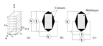
The important thing now is to consider the experiments, in
particular the geometry of the system and the way how the
contacts are made. We distinguish two different geometries :
the CIP geometry (current in the plane of the layers, see Fig. (1b))
and the CPP geometry (current perpendicular to the plane of the layers,
see Fig. (1c)).
FIG. 1.: (a) Schema of the unit
cell for a multilayer; (b) CIP geometry; (c) CPP geometry.
In CPP geometry, the current is perpendicular to the layers. Due
to current conservation, the perpendicular current is uniform
through the cell (i.e., J z l = J z superscript subscript 𝐽 𝑧 𝑙 subscript 𝐽 𝑧 J_{z}^{l}=J_{z} J z subscript 𝐽 𝑧 J_{z} J x l superscript subscript 𝐽 𝑥 𝑙 J_{x}^{l} J y l superscript subscript 𝐽 𝑦 𝑙 J_{y}^{l} J ¯ x ≡ ∑ l J x l / L subscript ¯ 𝐽 𝑥 subscript 𝑙 superscript subscript 𝐽 𝑥 𝑙 𝐿 \overline{J}_{x}\equiv\sum_{l}J_{x}^{l}/L J ¯ y ≡ ∑ l J y l / L subscript ¯ 𝐽 𝑦 subscript 𝑙 superscript subscript 𝐽 𝑦 𝑙 𝐿 \overline{J}_{y}\equiv\sum_{l}J_{y}^{l}/L ∇ × 𝐄 = 0 ∇ 𝐄 0 \nabla\times{\bf E}=0 E z l superscript subscript 𝐸 𝑧 𝑙 E_{z}^{l} 𝐄 𝐄 {\bf E} E x l = E x superscript subscript 𝐸 𝑥 𝑙 subscript 𝐸 𝑥 E_{x}^{l}=E_{x} E y l = E y superscript subscript 𝐸 𝑦 𝑙 subscript 𝐸 𝑦 E_{y}^{l}=E_{y} E x subscript 𝐸 𝑥 E_{x} E y subscript 𝐸 𝑦 E_{y} E z l superscript subscript 𝐸 𝑧 𝑙 E_{z}^{l} E ¯ z ≡ ∑ l E z l / L subscript ¯ 𝐸 𝑧 subscript 𝑙 superscript subscript 𝐸 𝑧 𝑙 𝐿 \overline{E}_{z}\equiv\sum_{l}E_{z}^{l}/L
By means of some
transformations on Eqs. (5 7 J x l superscript subscript 𝐽 𝑥 𝑙 J_{x}^{l} J y l superscript subscript 𝐽 𝑦 𝑙 J_{y}^{l} E z l superscript subscript 𝐸 𝑧 𝑙 E_{z}^{l} E x subscript 𝐸 𝑥 E_{x} E y subscript 𝐸 𝑦 E_{y} J z subscript 𝐽 𝑧 J_{z} 5
∑ l 2 σ z z l 1 l 2 E z l 2 = − ∑ l 2 σ z x l 1 l 2 E x l 2 − ∑ l 2 σ z y l 1 l 2 E y l 2 + J z l 1 . subscript subscript 𝑙 2 superscript subscript 𝜎 𝑧 𝑧 subscript 𝑙 1 subscript 𝑙 2 superscript subscript 𝐸 𝑧 subscript 𝑙 2 subscript subscript 𝑙 2 superscript subscript 𝜎 𝑧 𝑥 subscript 𝑙 1 subscript 𝑙 2 superscript subscript 𝐸 𝑥 subscript 𝑙 2 subscript subscript 𝑙 2 superscript subscript 𝜎 𝑧 𝑦 subscript 𝑙 1 subscript 𝑙 2 superscript subscript 𝐸 𝑦 subscript 𝑙 2 superscript subscript 𝐽 𝑧 subscript 𝑙 1 \displaystyle\sum_{l_{2}}\sigma_{zz}^{l_{1}l_{2}}E_{z}^{l_{2}}=-\sum_{l_{2}}\sigma_{zx}^{l_{1}l_{2}}E_{x}^{l_{2}}-\sum_{l_{2}}\sigma_{zy}^{l_{1}l_{2}}E_{y}^{l_{2}}+J_{z}^{l_{1}}. (8)
¿From Eq. (7
∑ l 2 ρ x x l 1 l 2 J x l 2 + ∑ l 2 ρ x y l 1 l 2 J y l 2 = E x l 1 − ∑ l 2 ρ x z l 1 l 2 J z l 2 , subscript subscript 𝑙 2 superscript subscript 𝜌 𝑥 𝑥 subscript 𝑙 1 subscript 𝑙 2 superscript subscript 𝐽 𝑥 subscript 𝑙 2 subscript subscript 𝑙 2 superscript subscript 𝜌 𝑥 𝑦 subscript 𝑙 1 subscript 𝑙 2 superscript subscript 𝐽 𝑦 subscript 𝑙 2 superscript subscript 𝐸 𝑥 subscript 𝑙 1 subscript subscript 𝑙 2 superscript subscript 𝜌 𝑥 𝑧 subscript 𝑙 1 subscript 𝑙 2 superscript subscript 𝐽 𝑧 subscript 𝑙 2 \displaystyle\sum_{l_{2}}\rho_{xx}^{l_{1}l_{2}}J_{x}^{l_{2}}+\sum_{l_{2}}\rho_{xy}^{l_{1}l_{2}}J_{y}^{l_{2}}=E_{x}^{l_{1}}-\sum_{l_{2}}\rho_{xz}^{l_{1}l_{2}}J_{z}^{l_{2}}, (9)
and
∑ l 2 ρ y x l 1 l 2 J x l 2 + ∑ l 2 ρ y y l 1 l 2 J y l 2 = E y l 1 − ∑ l 2 ρ y z l 1 l 2 J z l 2 . subscript subscript 𝑙 2 superscript subscript 𝜌 𝑦 𝑥 subscript 𝑙 1 subscript 𝑙 2 superscript subscript 𝐽 𝑥 subscript 𝑙 2 subscript subscript 𝑙 2 superscript subscript 𝜌 𝑦 𝑦 subscript 𝑙 1 subscript 𝑙 2 superscript subscript 𝐽 𝑦 subscript 𝑙 2 superscript subscript 𝐸 𝑦 subscript 𝑙 1 subscript subscript 𝑙 2 superscript subscript 𝜌 𝑦 𝑧 subscript 𝑙 1 subscript 𝑙 2 superscript subscript 𝐽 𝑧 subscript 𝑙 2 \displaystyle\sum_{l_{2}}\rho_{yx}^{l_{1}l_{2}}J_{x}^{l_{2}}+\sum_{l_{2}}\rho_{yy}^{l_{1}l_{2}}J_{y}^{l_{2}}=E_{y}^{l_{1}}-\sum_{l_{2}}\rho_{yz}^{l_{1}l_{2}}J_{z}^{l_{2}}. (10)
These three equations can be written under the matrix form
( ρ ~ x x ρ ~ x y 0 ρ ~ y x ρ ~ y y 0 0 0 σ ~ z z ) ( J ~ x J ~ y E ~ z ) subscript ~ 𝜌 𝑥 𝑥 subscript ~ 𝜌 𝑥 𝑦 0 subscript ~ 𝜌 𝑦 𝑥 subscript ~ 𝜌 𝑦 𝑦 0 0 0 subscript ~ 𝜎 𝑧 𝑧 subscript ~ 𝐽 𝑥 missing-subexpression missing-subexpression subscript ~ 𝐽 𝑦 missing-subexpression missing-subexpression subscript ~ 𝐸 𝑧 missing-subexpression missing-subexpression \displaystyle\left(\begin{array}[]{ccc}\tilde{\rho}_{xx}&\tilde{\rho}_{xy}&0\\
\tilde{\rho}_{yx}&\tilde{\rho}_{yy}&0\\
0&0&\tilde{\sigma}_{zz}\end{array}\right)\left(\begin{array}[]{lll}\tilde{J}_{x}\\
\tilde{J}_{y}\\
\tilde{E}_{z}\end{array}\right) (17)
= ( I ~ 0 − ρ ~ x z 0 I ~ − ρ ~ y z − σ ~ z x − σ ~ z y I ~ ) ( E ~ x E ~ y J ~ z ) , absent ~ 𝐼 0 subscript ~ 𝜌 𝑥 𝑧 0 ~ 𝐼 subscript ~ 𝜌 𝑦 𝑧 subscript ~ 𝜎 𝑧 𝑥 subscript ~ 𝜎 𝑧 𝑦 ~ 𝐼 subscript ~ 𝐸 𝑥 missing-subexpression missing-subexpression subscript ~ 𝐸 𝑦 missing-subexpression missing-subexpression subscript ~ 𝐽 𝑧 missing-subexpression missing-subexpression \displaystyle=\left(\begin{array}[]{ccc}\tilde{I}&0&-\tilde{\rho}_{xz}\\
0&\tilde{I}&-\tilde{\rho}_{yz}\\
-\tilde{\sigma}_{zx}&-\tilde{\sigma}_{zy}&\tilde{I}\end{array}\right)\left(\begin{array}[]{lll}\tilde{E}_{x}\\
\tilde{E}_{y}\\
\tilde{J}_{z}\end{array}\right), (24)
where I ~ ~ 𝐼 \tilde{I} ( L × L ) 𝐿 𝐿 (L\times L) A ~ i subscript ~ 𝐴 𝑖 \tilde{A}_{i} A = J 𝐴 𝐽 A=J E 𝐸 E ( L × L ) 𝐿 𝐿 (L\times L) a ~ i j subscript ~ 𝑎 𝑖 𝑗 \tilde{a}_{ij} a = σ 𝑎 𝜎 a=\sigma ρ 𝜌 \rho
A ~ i ≡ ( A i 1 ⋮ A i L ) , a ~ i j ≡ ( a i j 11 … a i j 1 L ⋮ ⋮ a i j L 1 … a i j L L ) . formulae-sequence subscript ~ 𝐴 𝑖 superscript subscript 𝐴 𝑖 1 missing-subexpression missing-subexpression ⋮ missing-subexpression missing-subexpression superscript subscript 𝐴 𝑖 𝐿 missing-subexpression missing-subexpression subscript ~ 𝑎 𝑖 𝑗 superscript subscript 𝑎 𝑖 𝑗 11 … superscript subscript 𝑎 𝑖 𝑗 1 𝐿 ⋮ missing-subexpression ⋮ superscript subscript 𝑎 𝑖 𝑗 𝐿 1 … superscript subscript 𝑎 𝑖 𝑗 𝐿 𝐿 \displaystyle\tilde{A}_{i}\equiv\left(\begin{array}[]{lll}A_{i}^{1}\\
\vdots\\
A_{i}^{L}\end{array}\right),\hskip 28.45274pt\tilde{a}_{ij}\equiv\left(\begin{array}[]{ccc}a_{ij}^{11}&\ldots&a_{ij}^{1L}\\
\vdots&&\vdots\\
a_{ij}^{L1}&\ldots&a_{ij}^{LL}\\
\end{array}\right). (31)
From Eq. (17
( J ~ x J ~ y E ~ z ) subscript ~ 𝐽 𝑥 missing-subexpression missing-subexpression subscript ~ 𝐽 𝑦 missing-subexpression missing-subexpression subscript ~ 𝐸 𝑧 missing-subexpression missing-subexpression \displaystyle\left(\begin{array}[]{lll}\tilde{J}_{x}\\
\tilde{J}_{y}\\
\tilde{E}_{z}\end{array}\right) = \displaystyle= ( ρ ~ x x ρ ~ x y 0 ρ ~ y x ρ ~ y y 0 0 0 σ ~ z z ) − 1 superscript subscript ~ 𝜌 𝑥 𝑥 subscript ~ 𝜌 𝑥 𝑦 0 subscript ~ 𝜌 𝑦 𝑥 subscript ~ 𝜌 𝑦 𝑦 0 0 0 subscript ~ 𝜎 𝑧 𝑧 1 \displaystyle\left(\begin{array}[]{ccc}\tilde{\rho}_{xx}&\tilde{\rho}_{xy}&0\\
\tilde{\rho}_{yx}&\tilde{\rho}_{yy}&0\\
0&0&\tilde{\sigma}_{zz}\end{array}\right)^{-1} (45)
× ( I ~ 0 − ρ ~ x z 0 I ~ − ρ ~ y z − σ ~ z x − σ ~ z y I ~ ) ( E x ~ E ~ y J ~ z ) . absent ~ 𝐼 0 subscript ~ 𝜌 𝑥 𝑧 0 ~ 𝐼 subscript ~ 𝜌 𝑦 𝑧 subscript ~ 𝜎 𝑧 𝑥 subscript ~ 𝜎 𝑧 𝑦 ~ 𝐼 ~ subscript 𝐸 𝑥 missing-subexpression missing-subexpression subscript ~ 𝐸 𝑦 missing-subexpression missing-subexpression subscript ~ 𝐽 𝑧 missing-subexpression missing-subexpression \displaystyle\times\left(\begin{array}[]{ccc}\tilde{I}&0&-\tilde{\rho}_{xz}\\
0&\tilde{I}&-\tilde{\rho}_{yz}\\
-\tilde{\sigma}_{zx}&-\tilde{\sigma}_{zy}&\tilde{I}\end{array}\right)\left(\begin{array}[]{lll}\tilde{E_{x}}\\
\tilde{E}_{y}\\
\tilde{J}_{z}\end{array}\right).
We inverse the first matrix in the r.s.h (it can be done
numerically) and perform the multiplication of the two matrices,
thus we get
( J ~ x J ~ y E ~ z ) subscript ~ 𝐽 𝑥 missing-subexpression missing-subexpression subscript ~ 𝐽 𝑦 missing-subexpression missing-subexpression subscript ~ 𝐸 𝑧 missing-subexpression missing-subexpression \displaystyle\left(\begin{array}[]{lll}\tilde{J}_{x}\\
\tilde{J}_{y}\\
\tilde{E}_{z}\end{array}\right) = \displaystyle= ( s ~ x x s ~ x y − ( s ~ x x ρ ~ x z + s ~ x y ρ ~ y z ) s ~ y x s ~ y y − ( s ~ y x ρ ~ x z + s ~ y y ρ ~ y z ) − p ~ z z σ ~ z x − p ~ z z σ ~ z y p ~ z z ) subscript ~ 𝑠 𝑥 𝑥 subscript ~ 𝑠 𝑥 𝑦 subscript ~ 𝑠 𝑥 𝑥 subscript ~ 𝜌 𝑥 𝑧 subscript ~ 𝑠 𝑥 𝑦 subscript ~ 𝜌 𝑦 𝑧 subscript ~ 𝑠 𝑦 𝑥 subscript ~ 𝑠 𝑦 𝑦 subscript ~ 𝑠 𝑦 𝑥 subscript ~ 𝜌 𝑥 𝑧 subscript ~ 𝑠 𝑦 𝑦 subscript ~ 𝜌 𝑦 𝑧 subscript ~ 𝑝 𝑧 𝑧 subscript ~ 𝜎 𝑧 𝑥 subscript ~ 𝑝 𝑧 𝑧 subscript ~ 𝜎 𝑧 𝑦 subscript ~ 𝑝 𝑧 𝑧 \displaystyle\left(\begin{array}[]{ccc}\tilde{s}_{xx}&\tilde{s}_{xy}&-(\tilde{s}_{xx}\tilde{\rho}_{xz}+\tilde{s}_{xy}\tilde{\rho}_{yz})\\
\tilde{s}_{yx}&\tilde{s}_{yy}&-(\tilde{s}_{yx}\tilde{\rho}_{xz}+\tilde{s}_{yy}\tilde{\rho}_{yz})\\
-\tilde{p}_{zz}\tilde{\sigma}_{zx}&-\tilde{p}_{zz}\tilde{\sigma}_{zy}&\tilde{p}_{zz}\\
\end{array}\right) (56)
× ( E ~ x E ~ y J ~ z ) , absent subscript ~ 𝐸 𝑥 missing-subexpression missing-subexpression subscript ~ 𝐸 𝑦 missing-subexpression missing-subexpression subscript ~ 𝐽 𝑧 missing-subexpression missing-subexpression \displaystyle\times\left(\begin{array}[]{lll}\tilde{E}_{x}\\
\tilde{E}_{y}\\
\tilde{J}_{z}\end{array}\right),
where s ~ i j subscript ~ 𝑠 𝑖 𝑗 \tilde{s}_{ij} p ~ z z subscript ~ 𝑝 𝑧 𝑧 \tilde{p}_{zz} ( L × L ) 𝐿 𝐿 (L\times L)
( s ~ x x s ~ x y 0 s ~ y x s ~ y y 0 0 0 p ~ z z ) ≡ ( ρ ~ x x ρ ~ x y 0 ρ ~ y x ρ ~ y y 0 0 0 σ ~ z z ) − 1 . subscript ~ 𝑠 𝑥 𝑥 subscript ~ 𝑠 𝑥 𝑦 0 subscript ~ 𝑠 𝑦 𝑥 subscript ~ 𝑠 𝑦 𝑦 0 0 0 subscript ~ 𝑝 𝑧 𝑧 superscript subscript ~ 𝜌 𝑥 𝑥 subscript ~ 𝜌 𝑥 𝑦 0 subscript ~ 𝜌 𝑦 𝑥 subscript ~ 𝜌 𝑦 𝑦 0 0 0 subscript ~ 𝜎 𝑧 𝑧 1 \displaystyle\left(\begin{array}[]{ccc}\tilde{s}_{xx}&\tilde{s}_{xy}&0\\
\tilde{s}_{yx}&\tilde{s}_{yy}&0\\
0&0&\tilde{p}_{zz}\end{array}\right)\equiv\left(\begin{array}[]{ccc}\tilde{\rho}_{xx}&\tilde{\rho}_{xy}&0\\
\tilde{\rho}_{yx}&\tilde{\rho}_{yy}&0\\
0&0&\tilde{\sigma}_{zz}\end{array}\right)^{-1}. (63)
By using the fact that E x subscript 𝐸 𝑥 E_{x} E y subscript 𝐸 𝑦 E_{y} J z subscript 𝐽 𝑧 J_{z} ( 3 L × 3 L ) 3 𝐿 3 𝐿 (3L\times 3L) 56 ( 3 L × 3 ) 3 𝐿 3 (3L\times 3)
( J x 1 ⋮ J x L J y 1 ⋮ J y L E z 1 ⋮ E z L ) = ( ∑ l 2 s x x 1 l 2 ∑ l 2 s x y 1 l 2 − ∑ l 2 , l 3 ( s x x 1 l 3 ρ x z l 3 l 2 + s x y 1 l 3 ρ y z l 3 l 2 ) ⋮ ⋮ ⋮ ∑ l 2 s x x L l 2 ∑ l 2 s x y L l 2 − ∑ l 2 , l 3 ( s x x L l 3 ρ x z l 3 l 2 + s x y L l 3 ρ x y l 3 l 2 ) ∑ l 2 s y x 1 l 2 ∑ l 2 s y y 1 l 2 − ∑ l 2 , l 3 ( s y x 1 l 3 ρ x z l 3 l 2 + s y y 1 l 3 ρ y z l 3 l 2 ) ⋮ ⋮ ⋮ ∑ l 2 s y x L l 2 ∑ l 2 s y y L l 2 − ∑ l 2 , l 3 ( s y x L l 3 ρ x z l 3 l 2 + s y y L l 3 ρ y z l 3 l 2 ) − ∑ l 2 , l 3 p z z 1 l 3 σ z x l 3 l 2 − ∑ l 2 , l 3 p z z 1 l 3 σ z y l 3 l 2 ∑ l 2 p z z 1 l 2 ⋮ ⋮ ⋮ − ∑ l 2 , l 3 p z z L l 3 σ z x l 3 l 2 − ∑ l 2 , l 3 p z z L l 3 σ z y l 3 l 2 ∑ l 2 p z z L l 2 ) ( E x E y J z ) . superscript subscript 𝐽 𝑥 1 missing-subexpression missing-subexpression missing-subexpression missing-subexpression missing-subexpression missing-subexpression missing-subexpression missing-subexpression ⋮ missing-subexpression missing-subexpression missing-subexpression missing-subexpression missing-subexpression missing-subexpression missing-subexpression missing-subexpression superscript subscript 𝐽 𝑥 𝐿 missing-subexpression missing-subexpression missing-subexpression missing-subexpression missing-subexpression missing-subexpression missing-subexpression missing-subexpression superscript subscript 𝐽 𝑦 1 missing-subexpression missing-subexpression missing-subexpression missing-subexpression missing-subexpression missing-subexpression missing-subexpression missing-subexpression ⋮ missing-subexpression missing-subexpression missing-subexpression missing-subexpression missing-subexpression missing-subexpression missing-subexpression missing-subexpression superscript subscript 𝐽 𝑦 𝐿 missing-subexpression missing-subexpression missing-subexpression missing-subexpression missing-subexpression missing-subexpression missing-subexpression missing-subexpression superscript subscript 𝐸 𝑧 1 missing-subexpression missing-subexpression missing-subexpression missing-subexpression missing-subexpression missing-subexpression missing-subexpression missing-subexpression ⋮ missing-subexpression missing-subexpression missing-subexpression missing-subexpression missing-subexpression missing-subexpression missing-subexpression missing-subexpression superscript subscript 𝐸 𝑧 𝐿 missing-subexpression missing-subexpression missing-subexpression missing-subexpression missing-subexpression missing-subexpression missing-subexpression missing-subexpression subscript subscript 𝑙 2 superscript subscript 𝑠 𝑥 𝑥 1 subscript 𝑙 2 subscript subscript 𝑙 2 superscript subscript 𝑠 𝑥 𝑦 1 subscript 𝑙 2 subscript subscript 𝑙 2 subscript 𝑙 3
superscript subscript 𝑠 𝑥 𝑥 1 subscript 𝑙 3 superscript subscript 𝜌 𝑥 𝑧 subscript 𝑙 3 subscript 𝑙 2 superscript subscript 𝑠 𝑥 𝑦 1 subscript 𝑙 3 superscript subscript 𝜌 𝑦 𝑧 subscript 𝑙 3 subscript 𝑙 2 missing-subexpression missing-subexpression missing-subexpression missing-subexpression missing-subexpression missing-subexpression ⋮ ⋮ ⋮ missing-subexpression missing-subexpression missing-subexpression missing-subexpression missing-subexpression missing-subexpression subscript subscript 𝑙 2 superscript subscript 𝑠 𝑥 𝑥 𝐿 subscript 𝑙 2 subscript subscript 𝑙 2 superscript subscript 𝑠 𝑥 𝑦 𝐿 subscript 𝑙 2 subscript subscript 𝑙 2 subscript 𝑙 3
superscript subscript 𝑠 𝑥 𝑥 𝐿 subscript 𝑙 3 superscript subscript 𝜌 𝑥 𝑧 subscript 𝑙 3 subscript 𝑙 2 superscript subscript 𝑠 𝑥 𝑦 𝐿 subscript 𝑙 3 superscript subscript 𝜌 𝑥 𝑦 subscript 𝑙 3 subscript 𝑙 2 missing-subexpression missing-subexpression missing-subexpression missing-subexpression missing-subexpression missing-subexpression subscript subscript 𝑙 2 superscript subscript 𝑠 𝑦 𝑥 1 subscript 𝑙 2 subscript subscript 𝑙 2 superscript subscript 𝑠 𝑦 𝑦 1 subscript 𝑙 2 subscript subscript 𝑙 2 subscript 𝑙 3
superscript subscript 𝑠 𝑦 𝑥 1 subscript 𝑙 3 superscript subscript 𝜌 𝑥 𝑧 subscript 𝑙 3 subscript 𝑙 2 superscript subscript 𝑠 𝑦 𝑦 1 subscript 𝑙 3 superscript subscript 𝜌 𝑦 𝑧 subscript 𝑙 3 subscript 𝑙 2 missing-subexpression missing-subexpression missing-subexpression missing-subexpression missing-subexpression missing-subexpression ⋮ ⋮ ⋮ missing-subexpression missing-subexpression missing-subexpression missing-subexpression missing-subexpression missing-subexpression subscript subscript 𝑙 2 superscript subscript 𝑠 𝑦 𝑥 𝐿 subscript 𝑙 2 subscript subscript 𝑙 2 superscript subscript 𝑠 𝑦 𝑦 𝐿 subscript 𝑙 2 subscript subscript 𝑙 2 subscript 𝑙 3
superscript subscript 𝑠 𝑦 𝑥 𝐿 subscript 𝑙 3 superscript subscript 𝜌 𝑥 𝑧 subscript 𝑙 3 subscript 𝑙 2 superscript subscript 𝑠 𝑦 𝑦 𝐿 subscript 𝑙 3 superscript subscript 𝜌 𝑦 𝑧 subscript 𝑙 3 subscript 𝑙 2 missing-subexpression missing-subexpression missing-subexpression missing-subexpression missing-subexpression missing-subexpression subscript subscript 𝑙 2 subscript 𝑙 3
superscript subscript 𝑝 𝑧 𝑧 1 subscript 𝑙 3 superscript subscript 𝜎 𝑧 𝑥 subscript 𝑙 3 subscript 𝑙 2 subscript subscript 𝑙 2 subscript 𝑙 3
superscript subscript 𝑝 𝑧 𝑧 1 subscript 𝑙 3 superscript subscript 𝜎 𝑧 𝑦 subscript 𝑙 3 subscript 𝑙 2 subscript subscript 𝑙 2 superscript subscript 𝑝 𝑧 𝑧 1 subscript 𝑙 2 missing-subexpression missing-subexpression missing-subexpression missing-subexpression missing-subexpression missing-subexpression ⋮ ⋮ ⋮ missing-subexpression missing-subexpression missing-subexpression missing-subexpression missing-subexpression missing-subexpression subscript subscript 𝑙 2 subscript 𝑙 3
superscript subscript 𝑝 𝑧 𝑧 𝐿 subscript 𝑙 3 superscript subscript 𝜎 𝑧 𝑥 subscript 𝑙 3 subscript 𝑙 2 subscript subscript 𝑙 2 subscript 𝑙 3
superscript subscript 𝑝 𝑧 𝑧 𝐿 subscript 𝑙 3 superscript subscript 𝜎 𝑧 𝑦 subscript 𝑙 3 subscript 𝑙 2 subscript subscript 𝑙 2 superscript subscript 𝑝 𝑧 𝑧 𝐿 subscript 𝑙 2 missing-subexpression missing-subexpression missing-subexpression missing-subexpression missing-subexpression missing-subexpression subscript 𝐸 𝑥 missing-subexpression missing-subexpression subscript 𝐸 𝑦 missing-subexpression missing-subexpression subscript 𝐽 𝑧 missing-subexpression missing-subexpression \displaystyle\left(\begin{array}[]{lllllllll}J_{x}^{1}\\
\vdots\\
J_{x}^{L}\\
J_{y}^{1}\\
\vdots\\
J_{y}^{L}\\
E_{z}^{1}\\
\vdots\\
E_{z}^{L}\end{array}\right)=\left(\begin{array}[]{ccccccccc}\sum_{l_{2}}s_{xx}^{1l_{2}}&\sum_{l_{2}}s_{xy}^{1l_{2}}&-\sum_{l_{2},l_{3}}\left(s_{xx}^{1l_{3}}\rho_{xz}^{l_{3}l_{2}}+s_{xy}^{1l_{3}}\rho_{yz}^{l_{3}l_{2}}\right)\\
\vdots&\vdots&\vdots\\
\sum_{l_{2}}s_{xx}^{Ll_{2}}&\sum_{l_{2}}s_{xy}^{Ll_{2}}&-\sum_{l_{2},l_{3}}\left(s_{xx}^{Ll_{3}}\rho_{xz}^{l_{3}l_{2}}+s_{xy}^{Ll_{3}}\rho_{xy}^{l_{3}l_{2}}\right)\\
\sum_{l_{2}}s_{yx}^{1l_{2}}&\sum_{l_{2}}s_{yy}^{1l_{2}}&-\sum_{l_{2},l_{3}}\left(s_{yx}^{1l_{3}}\rho_{xz}^{l_{3}l_{2}}+s_{yy}^{1l_{3}}\rho_{yz}^{l_{3}l_{2}}\right)\\
\vdots&\vdots&\vdots\\
\sum_{l_{2}}s_{yx}^{Ll_{2}}&\sum_{l_{2}}s_{yy}^{Ll_{2}}&-\sum_{l_{2},l_{3}}\left(s_{yx}^{Ll_{3}}\rho_{xz}^{l_{3}l_{2}}+s_{yy}^{Ll_{3}}\rho_{yz}^{l_{3}l_{2}}\right)\\
-\sum_{l_{2},l_{3}}p_{zz}^{1l_{3}}\sigma_{zx}^{l_{3}l_{2}}&-\sum_{l_{2},l_{3}}p_{zz}^{1l_{3}}\sigma_{zy}^{l_{3}l_{2}}&\sum_{l_{2}}p_{zz}^{1l_{2}}\\
\vdots&\vdots&\vdots\\
-\sum_{l_{2},l_{3}}p_{zz}^{Ll_{3}}\sigma_{zx}^{l_{3}l_{2}}&-\sum_{l_{2},l_{3}}p_{zz}^{Ll_{3}}\sigma_{zy}^{l_{3}l_{2}}&\sum_{l_{2}}p_{zz}^{Ll_{2}}\end{array}\right)\left(\begin{array}[]{lll}E_{x}\\
E_{y}\\
J_{z}\end{array}\right). (85)
As we are interested by the average currents
J ¯ x ≡ ∑ l J x l / L subscript ¯ 𝐽 𝑥 subscript 𝑙 superscript subscript 𝐽 𝑥 𝑙 𝐿 \overline{J}_{x}\equiv\sum_{l}J_{x}^{l}/L J ¯ y ≡ ∑ l J y l / L subscript ¯ 𝐽 𝑦 subscript 𝑙 superscript subscript 𝐽 𝑦 𝑙 𝐿 \overline{J}_{y}\equiv\sum_{l}J_{y}^{l}/L E ¯ z ≡ ∑ l E z l / L subscript ¯ 𝐸 𝑧 subscript 𝑙 superscript subscript 𝐸 𝑧 𝑙 𝐿 \overline{E}_{z}\equiv\sum_{l}E_{z}^{l}/L ( 3 L × 3 ) 3 𝐿 3 (3L\times 3) 85 ( 3 × 3 ) 3 3 (3\times 3)
( J ¯ x J ¯ y E ¯ z ) = ( ‖ s x x ‖ ‖ s x y ‖ − ‖ s x x ρ x z + s x y ρ y z ‖ ‖ s y x ‖ ‖ s y y ‖ − ‖ s y x ρ x z + s y y ρ y z ‖ − ‖ p z z σ z x ‖ − ‖ p z z σ z y ‖ ‖ p z z ‖ ) ( E x E y J z ) , subscript ¯ 𝐽 𝑥 missing-subexpression missing-subexpression subscript ¯ 𝐽 𝑦 missing-subexpression missing-subexpression subscript ¯ 𝐸 𝑧 missing-subexpression missing-subexpression norm subscript 𝑠 𝑥 𝑥 norm subscript 𝑠 𝑥 𝑦 norm subscript 𝑠 𝑥 𝑥 subscript 𝜌 𝑥 𝑧 subscript 𝑠 𝑥 𝑦 subscript 𝜌 𝑦 𝑧 norm subscript 𝑠 𝑦 𝑥 norm subscript 𝑠 𝑦 𝑦 norm subscript 𝑠 𝑦 𝑥 subscript 𝜌 𝑥 𝑧 subscript 𝑠 𝑦 𝑦 subscript 𝜌 𝑦 𝑧 norm subscript 𝑝 𝑧 𝑧 subscript 𝜎 𝑧 𝑥 norm subscript 𝑝 𝑧 𝑧 subscript 𝜎 𝑧 𝑦 norm subscript 𝑝 𝑧 𝑧 subscript 𝐸 𝑥 missing-subexpression missing-subexpression subscript 𝐸 𝑦 missing-subexpression missing-subexpression subscript 𝐽 𝑧 missing-subexpression missing-subexpression \displaystyle\left(\begin{array}[]{lll}\overline{J}_{x}\\
\overline{J}_{y}\\
\overline{E}_{z}\end{array}\right)=\left(\begin{array}[]{ccc}\|{s}_{xx}\|&\|{s}_{xy}\|&-\|{s}_{xx}{\rho}_{xz}+{s}_{xy}{\rho}_{yz}\|\\
\|{s}_{yx}\|&\|{s}_{yy}\|&-\|{s}_{yx}{\rho}_{xz}+{s}_{yy}{\rho}_{yz}\|\\
-\|{p}_{zz}{\sigma}_{zx}\|&-\|{p}_{zz}{\sigma}_{zy}\|&\|{p}_{zz}\|\\
\end{array}\right)\left(\begin{array}[]{lll}E_{x}\\
E_{y}\\
J_{z}\end{array}\right), (95)
where we have introduced the definition ‖ a i j ‖ ≡ ∑ l 1 , l 2 a i j l 1 l 2 / L norm subscript 𝑎 𝑖 𝑗 subscript subscript 𝑙 1 subscript 𝑙 2
superscript subscript 𝑎 𝑖 𝑗 subscript 𝑙 1 subscript 𝑙 2 𝐿 \|{a}_{ij}\|\equiv\sum_{l_{1},l_{2}}a_{ij}^{l_{1}l_{2}}/L
( 1 0 ‖ s x x ρ x z + s x y ρ y z ‖ 0 1 ‖ s y x ρ x z + s y y ρ y z ‖ 0 0 − ‖ p z z ‖ ) ( J ¯ x J ¯ y J z ) = ( ‖ s x x ‖ ‖ s x y ‖ 0 ‖ s y x ‖ ‖ s y y ‖ 0 − ‖ p z z σ z x ‖ − ‖ p z z σ z y ‖ − 1 ) ( E x E y E ¯ z ) . 1 0 norm subscript 𝑠 𝑥 𝑥 subscript 𝜌 𝑥 𝑧 subscript 𝑠 𝑥 𝑦 subscript 𝜌 𝑦 𝑧 0 1 norm subscript 𝑠 𝑦 𝑥 subscript 𝜌 𝑥 𝑧 subscript 𝑠 𝑦 𝑦 subscript 𝜌 𝑦 𝑧 0 0 norm subscript 𝑝 𝑧 𝑧 subscript ¯ 𝐽 𝑥 missing-subexpression missing-subexpression subscript ¯ 𝐽 𝑦 missing-subexpression missing-subexpression subscript 𝐽 𝑧 missing-subexpression missing-subexpression norm subscript 𝑠 𝑥 𝑥 norm subscript 𝑠 𝑥 𝑦 0 norm subscript 𝑠 𝑦 𝑥 norm subscript 𝑠 𝑦 𝑦 0 norm subscript 𝑝 𝑧 𝑧 subscript 𝜎 𝑧 𝑥 norm subscript 𝑝 𝑧 𝑧 subscript 𝜎 𝑧 𝑦 1 subscript 𝐸 𝑥 missing-subexpression missing-subexpression subscript 𝐸 𝑦 missing-subexpression missing-subexpression subscript ¯ 𝐸 𝑧 missing-subexpression missing-subexpression \displaystyle\left(\begin{array}[]{ccc}1&0&\|{s}_{xx}{\rho}_{xz}+{s}_{xy}{\rho}_{yz}\|\\
0&1&\|{s}_{yx}{\rho}_{xz}+{s}_{yy}{\rho}_{yz}\|\\
0&0&-\|{p}_{zz}\|\\
\end{array}\right)\left(\begin{array}[]{lll}\overline{J}_{x}\\
\overline{J}_{y}\\
J_{z}\end{array}\right)=\left(\begin{array}[]{ccc}\|{s}_{xx}\|&\|{s}_{xy}\|&0\\
\|{s}_{yx}\|&\|{s}_{yy}\|&0\\
-\|{p}_{zz}{\sigma}_{zx}\|&-\|{p}_{zz}{\sigma}_{zy}\|&-1\\
\end{array}\right)\left(\begin{array}[]{lll}E_{x}\\
E_{y}\\
\overline{E}_{z}\end{array}\right). (108)
From Eq. (108 σ ~ ~ 𝜎 \tilde{\sigma}
σ ¯ ¯ 𝜎 \displaystyle\overline{\sigma} = \displaystyle= ( 1 0 ‖ s x x ρ x z + s x y ρ y z ‖ 0 1 ‖ s y x ρ x z + s y y ρ y z ‖ 0 0 − ‖ p z z ‖ ) − 1 superscript 1 0 norm subscript 𝑠 𝑥 𝑥 subscript 𝜌 𝑥 𝑧 subscript 𝑠 𝑥 𝑦 subscript 𝜌 𝑦 𝑧 0 1 norm subscript 𝑠 𝑦 𝑥 subscript 𝜌 𝑥 𝑧 subscript 𝑠 𝑦 𝑦 subscript 𝜌 𝑦 𝑧 0 0 norm subscript 𝑝 𝑧 𝑧 1 \displaystyle\left(\begin{array}[]{ccc}1&0&\|{s}_{xx}{\rho}_{xz}+{s}_{xy}{\rho}_{yz}\|\\
0&1&\|{s}_{yx}{\rho}_{xz}+{s}_{yy}{\rho}_{yz}\|\\
0&0&-\|{p}_{zz}\|\\
\end{array}\right)^{-1} (116)
× ( ‖ s x x ‖ ‖ s x y ‖ 0 ‖ s y x ‖ ‖ s y y ‖ 0 − ‖ p z z σ z x ‖ − ‖ p z z σ z y ‖ − 1 ) . absent norm subscript 𝑠 𝑥 𝑥 norm subscript 𝑠 𝑥 𝑦 0 norm subscript 𝑠 𝑦 𝑥 norm subscript 𝑠 𝑦 𝑦 0 norm subscript 𝑝 𝑧 𝑧 subscript 𝜎 𝑧 𝑥 norm subscript 𝑝 𝑧 𝑧 subscript 𝜎 𝑧 𝑦 1 \displaystyle\times\left(\begin{array}[]{ccc}\|{s}_{xx}\|&\|{s}_{xy}\|&0\\
\|{s}_{yx}\|&\|{s}_{yy}\|&0\\
-\|{p}_{zz}{\sigma}_{zx}\|&-\|{p}_{zz}{\sigma}_{zy}\|&-1\\
\end{array}\right).
The inversion of the first matrix and the product of the two
matrices lead to the following expressions of the matrix elements
for the effective conductivity
σ ¯ x x subscript ¯ 𝜎 𝑥 𝑥 \displaystyle\overline{\sigma}_{xx} = \displaystyle= ‖ s x x ‖ − ‖ s x x ρ x z + s x y ρ y z ‖ ‖ p z z σ z x ‖ ‖ p z z ‖ , norm subscript 𝑠 𝑥 𝑥 norm subscript 𝑠 𝑥 𝑥 subscript 𝜌 𝑥 𝑧 subscript 𝑠 𝑥 𝑦 subscript 𝜌 𝑦 𝑧 norm subscript 𝑝 𝑧 𝑧 subscript 𝜎 𝑧 𝑥 norm subscript 𝑝 𝑧 𝑧 \displaystyle\|{s}_{xx}\|-\frac{\|{s}_{xx}{\rho}_{xz}+{s}_{xy}{\rho}_{yz}\|\|{p}_{zz}{\sigma}_{zx}\|}{\|{p}_{zz}\|}, (117)
σ ¯ x y subscript ¯ 𝜎 𝑥 𝑦 \displaystyle\overline{\sigma}_{xy} = \displaystyle= ‖ s x y ‖ − ‖ s x x ρ x z + s x y ρ y z ‖ ‖ p z z σ z y ‖ ‖ p z z ‖ , norm subscript 𝑠 𝑥 𝑦 norm subscript 𝑠 𝑥 𝑥 subscript 𝜌 𝑥 𝑧 subscript 𝑠 𝑥 𝑦 subscript 𝜌 𝑦 𝑧 norm subscript 𝑝 𝑧 𝑧 subscript 𝜎 𝑧 𝑦 norm subscript 𝑝 𝑧 𝑧 \displaystyle\|{s}_{xy}\|-\frac{\|{s}_{xx}{\rho}_{xz}+{s}_{xy}{\rho}_{yz}\|\|{p}_{zz}{\sigma}_{zy}\|}{\|{p}_{zz}\|}, (118)
σ ¯ x z subscript ¯ 𝜎 𝑥 𝑧 \displaystyle\overline{\sigma}_{xz} = \displaystyle= − ‖ s x x ρ x z + s x y ρ y z ‖ ‖ p z z ‖ , norm subscript 𝑠 𝑥 𝑥 subscript 𝜌 𝑥 𝑧 subscript 𝑠 𝑥 𝑦 subscript 𝜌 𝑦 𝑧 norm subscript 𝑝 𝑧 𝑧 \displaystyle-\frac{\|{s}_{xx}{\rho}_{xz}+{s}_{xy}{\rho}_{yz}\|}{\|{p}_{zz}\|}, (119)
σ ¯ y x subscript ¯ 𝜎 𝑦 𝑥 \displaystyle\overline{\sigma}_{yx} = \displaystyle= ‖ s y x ‖ − ‖ s y x ρ x z + s y y ρ y z ‖ ‖ p z z σ z x ‖ ‖ p z z ‖ , norm subscript 𝑠 𝑦 𝑥 norm subscript 𝑠 𝑦 𝑥 subscript 𝜌 𝑥 𝑧 subscript 𝑠 𝑦 𝑦 subscript 𝜌 𝑦 𝑧 norm subscript 𝑝 𝑧 𝑧 subscript 𝜎 𝑧 𝑥 norm subscript 𝑝 𝑧 𝑧 \displaystyle\|{s}_{yx}\|-\frac{\|{s}_{yx}{\rho}_{xz}+{s}_{yy}{\rho}_{yz}\|\|{p}_{zz}{\sigma}_{zx}\|}{\|{p}_{zz}\|}, (120)
σ ¯ y y subscript ¯ 𝜎 𝑦 𝑦 \displaystyle\overline{\sigma}_{yy} = \displaystyle= ‖ s y y ‖ − ‖ s y x ρ x z + s y y ρ y z ‖ ‖ p z z σ z y ‖ ‖ p z z ‖ , norm subscript 𝑠 𝑦 𝑦 norm subscript 𝑠 𝑦 𝑥 subscript 𝜌 𝑥 𝑧 subscript 𝑠 𝑦 𝑦 subscript 𝜌 𝑦 𝑧 norm subscript 𝑝 𝑧 𝑧 subscript 𝜎 𝑧 𝑦 norm subscript 𝑝 𝑧 𝑧 \displaystyle\|{s}_{yy}\|-\frac{\|{s}_{yx}{\rho}_{xz}+{s}_{yy}{\rho}_{yz}\|\|{p}_{zz}{\sigma}_{zy}\|}{\|{p}_{zz}\|}, (121)
σ ¯ y z subscript ¯ 𝜎 𝑦 𝑧 \displaystyle\overline{\sigma}_{yz} = \displaystyle= − ‖ s y x ρ x z + s y y ρ y z ‖ ‖ p z z ‖ , norm subscript 𝑠 𝑦 𝑥 subscript 𝜌 𝑥 𝑧 subscript 𝑠 𝑦 𝑦 subscript 𝜌 𝑦 𝑧 norm subscript 𝑝 𝑧 𝑧 \displaystyle-\frac{\|{s}_{yx}{\rho}_{xz}+{s}_{yy}{\rho}_{yz}\|}{\|{p}_{zz}\|}, (122)
σ ¯ z x subscript ¯ 𝜎 𝑧 𝑥 \displaystyle\overline{\sigma}_{zx} = \displaystyle= ‖ p z z σ z x ‖ ‖ p z z ‖ , norm subscript 𝑝 𝑧 𝑧 subscript 𝜎 𝑧 𝑥 norm subscript 𝑝 𝑧 𝑧 \displaystyle\frac{\|{p}_{zz}{\sigma}_{zx}\|}{\|{p}_{zz}\|}, (123)
σ ¯ z y subscript ¯ 𝜎 𝑧 𝑦 \displaystyle\overline{\sigma}_{zy} = \displaystyle= ‖ p z z σ z y ‖ ‖ p z z ‖ , norm subscript 𝑝 𝑧 𝑧 subscript 𝜎 𝑧 𝑦 norm subscript 𝑝 𝑧 𝑧 \displaystyle\frac{\|{p}_{zz}{\sigma}_{zy}\|}{\|{p}_{zz}\|}, (124)
σ ¯ z z subscript ¯ 𝜎 𝑧 𝑧 \displaystyle\overline{\sigma}_{zz} = \displaystyle= 1 ‖ p z z ‖ . 1 norm subscript 𝑝 𝑧 𝑧 \displaystyle\frac{1}{\|{p}_{zz}\|}. (125)
From Eq. (108 ρ ¯ ¯ 𝜌 \overline{\rho}
ρ ¯ = ( ‖ s x x ‖ ‖ s x y ‖ 0 ‖ s y x ‖ ‖ s y y ‖ 0 − ‖ p z z σ z x ‖ − ‖ p z z σ z y ‖ − 1 ) − 1 ¯ 𝜌 superscript norm subscript 𝑠 𝑥 𝑥 norm subscript 𝑠 𝑥 𝑦 0 norm subscript 𝑠 𝑦 𝑥 norm subscript 𝑠 𝑦 𝑦 0 norm subscript 𝑝 𝑧 𝑧 subscript 𝜎 𝑧 𝑥 norm subscript 𝑝 𝑧 𝑧 subscript 𝜎 𝑧 𝑦 1 1 \displaystyle\overline{\rho}=\left(\begin{array}[]{ccc}\|{s}_{xx}\|&\|{s}_{xy}\|&0\\
\|{s}_{yx}\|&\|{s}_{yy}\|&0\\
-\|{p}_{zz}{\sigma}_{zx}\|&-\|{p}_{zz}{\sigma}_{zy}\|&-1\\
\end{array}\right)^{-1} (129)
× ( 1 0 ‖ s x x ρ x z + s x y ρ y z ‖ 0 1 ‖ s y x ρ x z + s y y ρ y z ‖ 0 0 − ‖ p z z ‖ ) . absent 1 0 norm subscript 𝑠 𝑥 𝑥 subscript 𝜌 𝑥 𝑧 subscript 𝑠 𝑥 𝑦 subscript 𝜌 𝑦 𝑧 0 1 norm subscript 𝑠 𝑦 𝑥 subscript 𝜌 𝑥 𝑧 subscript 𝑠 𝑦 𝑦 subscript 𝜌 𝑦 𝑧 0 0 norm subscript 𝑝 𝑧 𝑧 \displaystyle\times\left(\begin{array}[]{ccc}1&0&\|{s}_{xx}{\rho}_{xz}+{s}_{xy}{\rho}_{yz}\|\\
0&1&\|{s}_{yx}{\rho}_{xz}+{s}_{yy}{\rho}_{yz}\|\\
0&0&-\|{p}_{zz}\|\\
\end{array}\right). (133)
The inversion of the first matrix and the product of the two
matrices lead to the following expressions of the matrix elements
for the effective resistivity
ρ ¯ x x subscript ¯ 𝜌 𝑥 𝑥 \displaystyle\overline{\rho}_{xx} = \displaystyle= 1 D ‖ s y y ‖ , 1 𝐷 norm subscript 𝑠 𝑦 𝑦 \displaystyle\frac{1}{D}\|{s}_{yy}\|, (134)
ρ ¯ x y subscript ¯ 𝜌 𝑥 𝑦 \displaystyle\overline{\rho}_{xy} = \displaystyle= − 1 D ‖ s x y ‖ , 1 𝐷 norm subscript 𝑠 𝑥 𝑦 \displaystyle-\frac{1}{D}\|{s}_{xy}\|, (135)
ρ ¯ x z subscript ¯ 𝜌 𝑥 𝑧 \displaystyle\overline{\rho}_{xz} = \displaystyle= 1 D ( ∥ s y y ∥ ∥ s x x ρ x z + s x y ρ y z ∥ \displaystyle\frac{1}{D}\left(\|{s}_{yy}\|\|{s}_{xx}{\rho}_{xz}+{s}_{xy}{\rho}_{yz}\|\right. (137)
− ∥ s x y ∥ ∥ s y x ρ x z + s y y ρ y z ∥ ) , \displaystyle-\left.\|{s}_{xy}\|\|{s}_{yx}{\rho}_{xz}+{s}_{yy}{\rho}_{yz}\|\right),
ρ ¯ y x subscript ¯ 𝜌 𝑦 𝑥 \displaystyle\overline{\rho}_{yx} = \displaystyle= − 1 D ‖ s y x ‖ , 1 𝐷 norm subscript 𝑠 𝑦 𝑥 \displaystyle-\frac{1}{D}\|{s}_{yx}\|, (138)
ρ ¯ y y subscript ¯ 𝜌 𝑦 𝑦 \displaystyle\overline{\rho}_{yy} = \displaystyle= 1 D ‖ s x x ‖ , 1 𝐷 norm subscript 𝑠 𝑥 𝑥 \displaystyle\frac{1}{D}\|{s}_{xx}\|, (139)
ρ ¯ y z subscript ¯ 𝜌 𝑦 𝑧 \displaystyle\overline{\rho}_{yz} = \displaystyle= 1 D ( ∥ s x x ∥ ∥ s y x ρ x z + s y y ρ y z ∥ \displaystyle\frac{1}{D}\left(\|{s}_{xx}\|\|{s}_{yx}{\rho}_{xz}+{s}_{yy}{\rho}_{yz}\|\right. (141)
− ∥ s y x ∥ ∥ s x x ρ x z + s x y ρ y z ∥ ) , \displaystyle-\left.\|{s}_{yx}\|\|{s}_{xx}{\rho}_{xz}+{s}_{xy}{\rho}_{yz}\|\right),
ρ ¯ z x subscript ¯ 𝜌 𝑧 𝑥 \displaystyle\overline{\rho}_{zx} = \displaystyle= 1 D ( ‖ s y x ‖ ‖ p z z σ z y ‖ − ‖ s y y ‖ ‖ p z z σ z x ‖ ) , 1 𝐷 norm subscript 𝑠 𝑦 𝑥 norm subscript 𝑝 𝑧 𝑧 subscript 𝜎 𝑧 𝑦 norm subscript 𝑠 𝑦 𝑦 norm subscript 𝑝 𝑧 𝑧 subscript 𝜎 𝑧 𝑥 \displaystyle\frac{1}{D}\left(\|{s}_{yx}\|\|{p}_{zz}{\sigma}_{zy}\|-\|{s}_{yy}\|\|{p}_{zz}{\sigma}_{zx}\|\right), (142)
ρ ¯ z y subscript ¯ 𝜌 𝑧 𝑦 \displaystyle\overline{\rho}_{zy} = \displaystyle= 1 D ( ‖ s x y ‖ ‖ p z z σ z x ‖ − ‖ s x x ‖ ‖ p z z σ z y ‖ ) , 1 𝐷 norm subscript 𝑠 𝑥 𝑦 norm subscript 𝑝 𝑧 𝑧 subscript 𝜎 𝑧 𝑥 norm subscript 𝑠 𝑥 𝑥 norm subscript 𝑝 𝑧 𝑧 subscript 𝜎 𝑧 𝑦 \displaystyle\frac{1}{D}\left(\|{s}_{xy}\|\|{p}_{zz}{\sigma}_{zx}\|-\|{s}_{xx}\|\|{p}_{zz}{\sigma}_{zy}\|\right), (143)
ρ ¯ z z subscript ¯ 𝜌 𝑧 𝑧 \displaystyle\overline{\rho}_{zz} = \displaystyle= ∥ p z z ∥ + 1 D ( ( ∥ s y x ∥ ∥ p z z σ z y ∥ − ∥ s y y ∥ ∥ p z z σ z x ∥ ) \displaystyle\|{p}_{zz}\|+\frac{1}{D}\left((\|{s}_{yx}\|\|{p}_{zz}{\sigma}_{zy}\|-\|{s}_{yy}\|\|{p}_{zz}{\sigma}_{zx}\|)\right. (147)
× ‖ s x x ρ x z + s x y ρ y z ‖ absent norm subscript 𝑠 𝑥 𝑥 subscript 𝜌 𝑥 𝑧 subscript 𝑠 𝑥 𝑦 subscript 𝜌 𝑦 𝑧 \displaystyle\times\|{s}_{xx}{\rho}_{xz}+{s}_{xy}{\rho}_{yz}\|\,
+ ( ‖ s x y ‖ ‖ p z z σ z x ‖ − ‖ s x x ‖ ‖ p z z σ z y ‖ ) norm subscript 𝑠 𝑥 𝑦 norm subscript 𝑝 𝑧 𝑧 subscript 𝜎 𝑧 𝑥 norm subscript 𝑠 𝑥 𝑥 norm subscript 𝑝 𝑧 𝑧 subscript 𝜎 𝑧 𝑦 \displaystyle+(\|{s}_{xy}\|\|{p}_{zz}{\sigma}_{zx}\|-\|{s}_{xx}\|\|{p}_{zz}{\sigma}_{zy}\|)
× ∥ s y x ρ x z + s y y ρ y z ∥ ) , \displaystyle\times\left.\|{s}_{yx}{\rho}_{xz}+{s}_{yy}{\rho}_{yz}\|\right),
where we have introduced the denominator D ≡ ‖ s x x ‖ ‖ s y y ‖ − ‖ s x y ‖ ‖ s y x ‖ 𝐷 norm subscript 𝑠 𝑥 𝑥 norm subscript 𝑠 𝑦 𝑦 norm subscript 𝑠 𝑥 𝑦 norm subscript 𝑠 𝑦 𝑥 D\equiv\|{s}_{xx}\|\|{s}_{yy}\|-\|{s}_{xy}\|\|{s}_{yx}\| 117 134
Without magnetization and for a cubic lattice, the symmetry
imposes σ i ≠ j l 1 l 2 = ρ i ≠ j l 1 l 2 = 0 superscript subscript 𝜎 𝑖 𝑗 subscript 𝑙 1 subscript 𝑙 2 superscript subscript 𝜌 𝑖 𝑗 subscript 𝑙 1 subscript 𝑙 2 0 \sigma_{i\neq j}^{l_{1}l_{2}}=\rho_{i\neq j}^{l_{1}l_{2}}=0 s i i l 1 l 2 = σ i i l 1 l 2 superscript subscript 𝑠 𝑖 𝑖 subscript 𝑙 1 subscript 𝑙 2 superscript subscript 𝜎 𝑖 𝑖 subscript 𝑙 1 subscript 𝑙 2 s_{ii}^{l_{1}l_{2}}=\sigma_{ii}^{l_{1}l_{2}} i ∈ { x , y } 𝑖 𝑥 𝑦 i\in\{x,y\} p z z l 1 l 2 = ρ z z l 1 l 2 superscript subscript 𝑝 𝑧 𝑧 subscript 𝑙 1 subscript 𝑙 2 superscript subscript 𝜌 𝑧 𝑧 subscript 𝑙 1 subscript 𝑙 2 p_{zz}^{l_{1}l_{2}}=\rho_{zz}^{l_{1}l_{2}} 63 116 129
σ ¯ ¯ 𝜎 \displaystyle\overline{\sigma} = \displaystyle= ( ‖ σ x x ‖ 0 0 0 ‖ σ y y ‖ 0 0 0 1 ‖ ρ z z ‖ ) , norm subscript 𝜎 𝑥 𝑥 0 0 0 norm subscript 𝜎 𝑦 𝑦 0 0 0 1 norm subscript 𝜌 𝑧 𝑧 \displaystyle\left(\begin{array}[]{ccc}\|{\sigma}_{xx}\|&0&0\\
0&\|{\sigma}_{yy}\|&0\\
0&0&\frac{1}{{\|{\rho}}_{zz}\|}\end{array}\right), (151)
ρ ¯ ¯ 𝜌 \displaystyle\overline{\rho} = \displaystyle= ( 1 ‖ σ x x ‖ 0 0 0 1 ‖ σ y y ‖ 0 0 0 ‖ ρ z z ‖ ) . 1 norm subscript 𝜎 𝑥 𝑥 0 0 0 1 norm subscript 𝜎 𝑦 𝑦 0 0 0 norm subscript 𝜌 𝑧 𝑧 \displaystyle\left(\begin{array}[]{ccc}\frac{1}{\|{\sigma}_{xx}\|}&0&0\\
0&\frac{1}{\|{\sigma}_{yy}\|}&0\\
0&0&\|{\rho}_{zz}\|\end{array}\right). (155)
When the magnetization is along the x-direction, we have
σ i x l 1 l 2 = σ x i l 1 l 2 = ρ i x l 1 l 2 = ρ x i l 1 l 2 = 0 superscript subscript 𝜎 𝑖 𝑥 subscript 𝑙 1 subscript 𝑙 2 superscript subscript 𝜎 𝑥 𝑖 subscript 𝑙 1 subscript 𝑙 2 superscript subscript 𝜌 𝑖 𝑥 subscript 𝑙 1 subscript 𝑙 2 superscript subscript 𝜌 𝑥 𝑖 subscript 𝑙 1 subscript 𝑙 2 0 \sigma_{ix}^{l_{1}l_{2}}=\sigma_{xi}^{l_{1}l_{2}}=\rho_{ix}^{l_{1}l_{2}}=\rho_{xi}^{l_{1}l_{2}}=0 i ∈ { y , z } 𝑖 𝑦 𝑧 i\in\{y,z\} s i j l 1 l 2 superscript subscript 𝑠 𝑖 𝑗 subscript 𝑙 1 subscript 𝑙 2 s_{ij}^{l_{1}l_{2}} σ i j l 1 l 2 superscript subscript 𝜎 𝑖 𝑗 subscript 𝑙 1 subscript 𝑙 2 \sigma_{ij}^{l_{1}l_{2}} p i j l 1 l 2 superscript subscript 𝑝 𝑖 𝑗 subscript 𝑙 1 subscript 𝑙 2 p_{ij}^{l_{1}l_{2}} ρ i j l 1 l 2 superscript subscript 𝜌 𝑖 𝑗 subscript 𝑙 1 subscript 𝑙 2 \rho_{ij}^{l_{1}l_{2}}
σ ¯ ¯ 𝜎 \displaystyle\overline{\sigma} = \displaystyle= ( ‖ s x x ‖ 0 0 0 ‖ s y y ‖ − ‖ s y y ρ y z ‖ ‖ p z z σ z y ‖ ‖ p z z ‖ − ‖ s y y ρ y z ‖ ‖ p z z ‖ 0 ‖ p z z σ z y ‖ ‖ p z z ‖ 1 ‖ p z z ‖ ) , norm subscript 𝑠 𝑥 𝑥 0 0 0 norm subscript 𝑠 𝑦 𝑦 norm subscript 𝑠 𝑦 𝑦 subscript 𝜌 𝑦 𝑧 norm subscript 𝑝 𝑧 𝑧 subscript 𝜎 𝑧 𝑦 norm subscript 𝑝 𝑧 𝑧 norm subscript 𝑠 𝑦 𝑦 subscript 𝜌 𝑦 𝑧 norm subscript 𝑝 𝑧 𝑧 0 norm subscript 𝑝 𝑧 𝑧 subscript 𝜎 𝑧 𝑦 norm subscript 𝑝 𝑧 𝑧 1 norm subscript 𝑝 𝑧 𝑧 \displaystyle\left(\begin{array}[]{ccc}\|{s}_{xx}\|&0&0\\
0&\|{s}_{yy}\|-\frac{\|{s}_{yy}{\rho}_{yz}\|\|{p}_{zz}{\sigma}_{zy}\|}{\|{p}_{zz}\|}&-\frac{\|{s}_{yy}{\rho}_{yz}\|}{\|{p}_{zz}\|}\\
0&\frac{\|{p}_{zz}{\sigma}_{zy}\|}{\|{p}_{zz}\|}&\frac{1}{\|{p}_{zz}\|}\end{array}\right), (159)
ρ ¯ ¯ 𝜌 \displaystyle\overline{\rho} = \displaystyle= ( 1 ‖ s x x ‖ 0 0 0 1 ‖ s y y ‖ ‖ s y y ρ y z ‖ ‖ s y y ‖ 0 − ‖ p z z σ z y ‖ ‖ s y y ‖ ‖ p z z ‖ − ‖ s y y ρ y z ‖ ‖ p z z σ z y ‖ ‖ s y y ‖ ) , 1 norm subscript 𝑠 𝑥 𝑥 0 0 0 1 norm subscript 𝑠 𝑦 𝑦 norm subscript 𝑠 𝑦 𝑦 subscript 𝜌 𝑦 𝑧 norm subscript 𝑠 𝑦 𝑦 0 norm subscript 𝑝 𝑧 𝑧 subscript 𝜎 𝑧 𝑦 norm subscript 𝑠 𝑦 𝑦 norm subscript 𝑝 𝑧 𝑧 norm subscript 𝑠 𝑦 𝑦 subscript 𝜌 𝑦 𝑧 norm subscript 𝑝 𝑧 𝑧 subscript 𝜎 𝑧 𝑦 norm subscript 𝑠 𝑦 𝑦 \displaystyle\left(\begin{array}[]{ccc}\frac{1}{\|{s}_{xx}\|}&0&0\\
0&\frac{1}{\|{s}_{yy}\|}&\frac{\|{s}_{yy}{\rho}_{yz}\|}{\|{s}_{yy}\|}\\
0&-\frac{\|{p}_{zz}{\sigma}_{zy}\|}{\|{s}_{yy}\|}&\|{p}_{zz}\|-\frac{\|{s}_{yy}{\rho}_{yz}\|\|{p}_{zz}{\sigma}_{zy}\|}{\|{s}_{yy}\|}\end{array}\right), (163)
where D = ‖ s x x ‖ ‖ s y y ‖ 𝐷 norm subscript 𝑠 𝑥 𝑥 norm subscript 𝑠 𝑦 𝑦 D=\|{s}_{xx}\|\|{s}_{yy}\| 159 163
When the magnetization is along the z-direction, we have
σ i z l 1 l 2 = σ z i l 1 l 2 = ρ i z l 1 l 2 = ρ z i l 1 l 2 = 0 superscript subscript 𝜎 𝑖 𝑧 subscript 𝑙 1 subscript 𝑙 2 superscript subscript 𝜎 𝑧 𝑖 subscript 𝑙 1 subscript 𝑙 2 superscript subscript 𝜌 𝑖 𝑧 subscript 𝑙 1 subscript 𝑙 2 superscript subscript 𝜌 𝑧 𝑖 subscript 𝑙 1 subscript 𝑙 2 0 \sigma_{iz}^{l_{1}l_{2}}=\sigma_{zi}^{l_{1}l_{2}}=\rho_{iz}^{l_{1}l_{2}}=\rho_{zi}^{l_{1}l_{2}}=0 i ∈ { x , y } 𝑖 𝑥 𝑦 i\in\{x,y\} s i j l 1 l 2 = σ i j l 1 l 2 superscript subscript 𝑠 𝑖 𝑗 subscript 𝑙 1 subscript 𝑙 2 superscript subscript 𝜎 𝑖 𝑗 subscript 𝑙 1 subscript 𝑙 2 s_{ij}^{l_{1}l_{2}}=\sigma_{ij}^{l_{1}l_{2}} { i , j } ∈ { x , y } 𝑖 𝑗 𝑥 𝑦 \{i,j\}\in\{x,y\} p z z l 1 l 2 = ρ z z l 1 l 2 superscript subscript 𝑝 𝑧 𝑧 subscript 𝑙 1 subscript 𝑙 2 superscript subscript 𝜌 𝑧 𝑧 subscript 𝑙 1 subscript 𝑙 2 p_{zz}^{l_{1}l_{2}}=\rho_{zz}^{l_{1}l_{2}} 63
σ ¯ ¯ 𝜎 \displaystyle\overline{\sigma} = \displaystyle= ( ‖ σ x x ‖ ‖ σ x y ‖ 0 ‖ σ y x ‖ ‖ σ y y ‖ 0 0 0 1 ‖ ρ z z ‖ ) , norm subscript 𝜎 𝑥 𝑥 norm subscript 𝜎 𝑥 𝑦 0 norm subscript 𝜎 𝑦 𝑥 norm subscript 𝜎 𝑦 𝑦 0 0 0 1 norm subscript 𝜌 𝑧 𝑧 \displaystyle\left(\begin{array}[]{ccc}\|{\sigma}_{xx}\|&\|{\sigma}_{xy}\|&0\\
\|{\sigma}_{yx}\|&\|{\sigma}_{yy}\|&0\\
0&0&\frac{1}{\|{\rho}_{zz}\|}\end{array}\right), (167)
ρ ¯ ¯ 𝜌 \displaystyle\overline{\rho} = \displaystyle= ( 1 D ‖ σ y y ‖ − 1 D ‖ σ x y ‖ 0 − 1 D ‖ σ y x ‖ 1 D ‖ σ x x ‖ 0 0 0 ‖ ρ z z ‖ ) , 1 𝐷 norm subscript 𝜎 𝑦 𝑦 1 𝐷 norm subscript 𝜎 𝑥 𝑦 0 1 𝐷 norm subscript 𝜎 𝑦 𝑥 1 𝐷 norm subscript 𝜎 𝑥 𝑥 0 0 0 norm subscript 𝜌 𝑧 𝑧 \displaystyle\left(\begin{array}[]{ccc}\frac{1}{D}\|{\sigma}_{yy}\|&-\frac{1}{D}\|{\sigma}_{xy}\|&0\\
-\frac{1}{D}\|{\sigma}_{yx}\|&\frac{1}{D}\|{\sigma}_{xx}\|&0\\
0&0&\|{\rho}_{zz}\|\end{array}\right), (171)
where D = ‖ σ x x ‖ ‖ σ y y ‖ − ‖ σ x y ‖ ‖ σ y x ‖ 𝐷 norm subscript 𝜎 𝑥 𝑥 norm subscript 𝜎 𝑦 𝑦 norm subscript 𝜎 𝑥 𝑦 norm subscript 𝜎 𝑦 𝑥 D=\|{\sigma}_{xx}\|\|{\sigma}_{yy}\|-\|{\sigma}_{xy}\|\|{\sigma}_{yx}\| σ ¯ i j subscript ¯ 𝜎 𝑖 𝑗 \overline{\sigma}_{ij} { i , j } ∈ { x , y } 𝑖 𝑗 𝑥 𝑦 \{i,j\}\in\{x,y\} ‖ σ i j ‖ = ∑ l 1 , l 2 σ i j l 1 , l 2 / L norm subscript 𝜎 𝑖 𝑗 subscript subscript 𝑙 1 subscript 𝑙 2
superscript subscript 𝜎 𝑖 𝑗 subscript 𝑙 1 subscript 𝑙 2
𝐿 \|{\sigma}_{ij}\|=\sum_{l_{1},l_{2}}{\sigma}_{ij}^{l_{1},l_{2}}/L σ ¯ z z subscript ¯ 𝜎 𝑧 𝑧 \overline{\sigma}_{zz} 1 / ‖ ρ z z ‖ = 1 / ( ∑ l 1 , l 2 ρ z z l 1 , l 2 / L ) 1 norm subscript 𝜌 𝑧 𝑧 1 subscript subscript 𝑙 1 subscript 𝑙 2
superscript subscript 𝜌 𝑧 𝑧 subscript 𝑙 1 subscript 𝑙 2
𝐿 1/\|{\rho}_{zz}\|=1/(\sum_{l_{1},l_{2}}{\rho}_{zz}^{l_{1},l_{2}}/L) [3 , 6 , 7 ] .
Assuming the local limit, it is thus possible to model the
multilayer as a network of resistors in series (in the CIP
geometry) or in parallels (in the CPP
geometry)[3 , 8 ] .
* Corresponding author; present address: Centre de Physique Théorique, Luminy, Case 907, 13288 Marseille cedex 9, France; e-mail: crepieux@cpt.univ-mrs.fr
REFERENCES
[1]
G.D. Mahan, Many-Particle Physics (Plenum Press, New-York,
1990).
[2]
R. Kubo, Can. J. Phys. 34 , 1274 (1956); J. Phys. Soc. Jpn.
12 , 570 (1957).
[3]
H. Camblong, S. Zhang and P.L. Levy,
Phys. Rev. B 47 , 4735 (1993).
[4]
P.L. Levy, Solids State Physics , Vol. 47, edited by F. Seitz and D.
Turnbull (Plenum Press, 1994), p.367.
[5]
W.H. Butler, X.-G. Zhang, D.M.C. Nicholson and J.M. MacLaren, Phys. Rev. B 52 , 13399
(1995).
[6]
S. Zhang, Phys. Rev. B 51 , 3632
(1995).
[7]
C. Blaas, P. Weinberger, L. Szunyogh, P.M. Levy and C.B. Sommers,
Phys. Rev. B 60 , 492 (1999).
[8]
T. Valet and A. Fert, Phys. Rev. B 48 , 7099
(1993).