Propagation of waves in metallic photonic crystals at low frequencies and some theoretical aspects of left-handed materials

Abstract

An analytical theory of low frequency electromagnetic waves in metallic photonic crystals with a small volume fraction of a metal is presented. The evidence of the existence of such waves has been found recently via experiments and computations. We have obtained an exact dispersion equation for $\omega(k)$ and studied the cutoff frequency $\omega_{0}=\omega(0)$ as a function of parameters of the photonic crystal. An analytical expression for the permittivity $\epsilon$ is calculated. It is shown, that if the crystal is embedded into a medium with negative $\mu$, it has no propagating modes at any frequency. Thus, such a compound system is not a left-handed material (LHM). The recent experimental results on the LHM are discussed.

, ,

Veselago has shown[1] that if in some frequency range both permittivity $\epsilon$ and permeability $\mu$ are negative, the electromagnetic waves (EMW’s) propagate but they have some peculiar properties, from which the primary one is that vectors k, E, H form rather a left-handed than a right-handed triple of vectors. Materials, with this property are named left-handed materials (LHM).

The San Diego group[2] uses metallic photonic crystals (MPC’s) as a technological base for the LHM in the GHz frequency range. This idea comes from the pioneering computational and experimental studies of a few groups[3, 4, 5, 6, 7] which have found very low frequency EMW’s in the MPC. These EMW’s propagate above a very low cutoff frequency for which various groups obtained different values. Since the parameters of the MPC’s were also different, it was not clear whether or not the physics of these modes is the same. The suggested interpretations are very controversial. The group of Soukoulis[5] qualitatively interpreted the effect of propagation in terms of waveguide modes, while the group of Pendry[6] presented a completely original physical picture based upon a new longitudinal mode, called “plasma mode”. According to Pendry et al.[6] the resulting effective permittivity has a plasma-like behavior

$$\frac{\epsilon}{\epsilon_{0}}=1-\frac{\omega_{p}^{2}}{\omega(\omega+i\Gamma)},$$ (1)

however, expression for the “plasma” frequency contains the velocity of light and has a form

$$\omega_{p}^{2}=\frac{2\pi c^{2}}{d^{2}\ln(d/R)},\Gamma=\frac{\epsilon_{0}d^{2}\omega_{p}^{2}}{\pi R^{2}\sigma},$$ (2)

where $d$ is the lattice constant, $R$ is the radius of the metallic wires, $\sigma$ is the static conductivity of the metal. The same results for $\epsilon$ and $\omega_{p}$ have been later obtained theoretically by Sarychev and Shalaev[8].

The San Diego group accepted the “plasma model” and considered the negative $\epsilon$ at $\omega<\omega_{p}$ as one of the two crucial conditions for creation of the LHM. They have reported the first observation of the anomalous transmission and negative refraction in a compound system of split ring resonators (SRR’s) and MPC[2, 9]. According to Pendry et al.[10] such resonators create a negative bulk magnetic permeability due to the anomalous dispersion.

In this paper we present an analytical theory of the EMW’s propagating in the MPC without SRR’s at very low frequencies. The theory is based upon the parameters $f\ll 1$ and $\omega R/c\ll 1$, where $f$ is the volume fraction of a metal in the MPC. First we derive an exact dispersion equation for the s-polarized EMW in the system of infinite parallel thin straight wires ordered in a square lattice. The electric field of the wave is directed along the wires (z-axis), while the wave vector ${\bf k}$ is in the $x$-$y$ plane. Assume that the total current in each wire is $I_{0}\exp[-i(\omega t-{\bf k\cdot r}_{i})]$, where ${\bf r}_{i}$ is a two-dimensional radius-vector of the wire in the $x$-$y$ plane. The external solution for electric field $E_{z}$ of one wire, located at ${\bf r}_{i}=0$, has a form

$$E_{z}^{i}=\frac{I_{0}\mu_{0}\omega}{4}H^{(2)}_{0}\left(\frac{\omega}{c}\rho\right),$$ (3)

where $H^{(2)}_{0}=J_{0}-iN_{0}$ is the Hankel function which decays exponentially at ${\rm Im}\omega<0$. Neither $J_{0}$ nor $N_{0}$ has this important property. Here and below we omit the time dependent factor. The solution is written in cylindrical coordinates $z,\rho,\phi$ and it satisfies the boundary condition $B_{\phi}=(i/\omega)dE_{z}/d\rho=I_{0}\mu_{0}/2\pi\rho$ at $\rho=R$.

The electric field created by all wires is

$$E_{z}({\bf r})=\frac{I_{0}\mu_{0}\omega}{4}e^{i{\bf k\cdot r}}\sum_{j}e^{i{{\bf k\cdot}({\bf r}_{j}-{\bf r})}}H^{(2)}_{0}(\frac{\omega}{c}\rho_{j}),$$ (4)

where $\rho_{j}=\sqrt{(x-x_{j})^{2}+(y-y_{j})^{2}}$, summation is over all sites of the square lattice and the sum is a periodic function of ${\bf r}$. The dispersion equation follows from the boundary condition[11] that relates the total electric field at the surface of any wire $l$ to the total current through the wire $E_{z}(R)=I_{0}\exp{(i{\bf k}\cdot{\bf r}_{l})}/\sigma_{ef}\pi R^{2}$, where $\sigma_{ef}=2\sigma J_{1}(\kappa R)/\kappa RJ_{0}(\kappa R)$, $\kappa=(1+i)/\delta$, and $\delta$ is the skin depth. At small frequencies, when $\delta>R$ one gets $\sigma_{ef}\approx\sigma$. At high frequencies, when $\delta\leq 0.1R$, one gets the Rayleigh formula $\sigma_{ef}\approx(1+i)\sigma\delta/R$.

Note, that the EMW exists mostly if the skin-effect in the wires is strong. Using Eqs.(1,2) one can show that $\Gamma/\omega_{p}=\delta^{2}/(R^{2}\ln{d/R})$, where $\delta$ is the skin depth at $\omega=\omega_{p}$ (see also Ref.[12]). Thus, with the logarithmic accuracy one can say that $\Gamma\ll\omega_{p}$ if $\delta\ll R$. We show below that the exact solution has similar properties.

Finally, the dispersion equation for $\omega({\bf k})\equiv(\chi-i\gamma)c/d$ has a form

$$(\chi-i\gamma)\sum_{l,m}e^{id(k_{x}l+k_{y}m)}H_{0}^{(2)}(z_{lm})=\frac{4c\epsilon_{0}}{d\sigma_{ef}f},$$ (5)

where where $z_{lm}=(\chi-i\gamma)\sqrt{l^{2}+m^{2}+(R/d)^{2}}$, $l$ and $m$ are integer numbers and the small term $(R/d)^{2}$ under the square root is important only when $l=m=0$. Taking real and imaginary parts of Eq.(5) one gets two equations for $\chi$ and $\gamma$.

Now we study the cutoff frequency for the EMW’s $\omega_{0}$, which is the solution of Eq.(5) at $|{\bf k}|=0$:

$$(\chi-i\gamma)\sum_{l,m}H_{0}^{(2)}(z_{lm})=\frac{4c\epsilon_{0}}{d\sigma_{ef}f}.$$ (6)

The numerical results for the real part of the frequency are shown in Fig. 1. One can see that $\chi$ is of the order of few units. The values of $\gamma$ are of the order of the right hand side of Eq.(6). Thus, $\chi\gg\gamma$ if $f\sigma_{ef}/\epsilon_{0}\omega\gg 1$.

In addition to the numerical solution we propose an approximation valid at a very small $f$, when $|\ln f|\gg 1$. We separate the term with $l=m=0$ in Eq.(6) and substitute the rest of the sum by the integral. Then

$$(\chi-i\gamma)\left[\frac{2i}{\pi}\left(\ln{\frac{2}{\chi\sqrt{f/\pi}}}-{\bf C}\right)-\frac{4i}{(\chi-i\gamma)^{2}}\right]=\frac{4c\epsilon_{0}}{d\sigma_{ef}(\chi)f},$$ (7)

where we assume that $\gamma\ll\chi$. Here ${\bf C}$ is the Euler’s constant.

Figure 1 compares our result for the real part of the cutoff frequency given by Eq.(6) with the results given by Eqs.(2,7). In these calculations we assume that $\sigma_{ef}$ is given by the Rayleigh formula so that the right hand side of Eqs.(6,7) has a form $\alpha(1-i)\sqrt{\chi}$, where $\alpha=2c\epsilon_{0}R/fd\sigma\delta$ and $\delta$ is taken at $\omega=c/d$. One can see from Fig.1 that approximation Eq.(7) is much better than approximation Eq.(2). Both approximations coincide at small $f$ and they are accurate at extremely low values of $f$ ($\sim 10^{-7}$) when the logarithmic term in Eqs.(2,7) is very large. The computational and experimental data of Refs.[5, 9] are also shown at Fig. 1 and they are in a good agreement with Eq.(6). The result of Pendry group [6] for the cutoff frequency is $8.2{\rm\ GHz}$, while Eq.(6) gives $8.6{\rm\ GHz}$. Experimental result of Bayindir et al.[13] is $11.67{\rm\ GHz}$ while our Eq.(6) gives $11.8{\rm\ GHz}$. Thus, we can make a conclusion that the San Diego group, group of Pendry and Soukoulis group discuss the same mode but at different values of parameters and that our analytical theory describes the same mode as well.

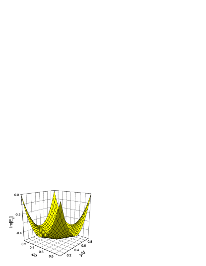
Figure 2: Imaginary part of the electric field inside the lattice cell in the units of $I_{0}\mu_{0}c/d$. The radius of the wires $R=0.8$ mm, the lattice constant $d=8$ mm, the static conductivity of the metal of the wires $\sigma=5.88\cdot 10^{7}$ ($\Omega\ \cdot$ m)^-1.

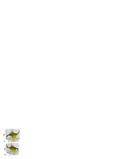
Figure 3: Real part of the $x$-($a$), and $y$-component(b) of the magnetic induction ${\bf B}$ inside the lattice cell in the units of $I_{0}\mu_{0}/d$. The radius of the wires $R=0.8$ mm, the lattice constant $d=8$ mm, the static conductivity of the metal of the wires $\sigma=5.88\cdot 10^{7}$ ($\Omega\ \cdot$ m)^-1.

At Fig. 2 we plot the imaginary part of the $z$-component of the electric field in the unit cell as calculated from Eq.(4) with $k=0$. Real parts of the $x$- and $y$- components of the magnetic induction, are shown in Fig. 3. Real part of the $E_{z}$ and imaginary parts of $B_{x}$, $B_{y}$ are much smaller than imaginary part of $E_{z}$ and real part of $B_{x}$, $B_{y}$ correspondingly if $\gamma\ll 1$. As one can see, the fields are strongly modulated inside the lattice cell and $E_{z}$ is close to zero near each wire so that absorption is small. This fact allows the low frequency mode propagate in the MPC under the condition $f\sigma_{ef}/\epsilon_{0}\omega\gg 1$.

Now we find the component of electric permittivity $\epsilon(\omega)=\epsilon_{zz}$, which describes the s-polarized extraordinary waves in the uniaxial crystal. It is defined by the relation $\epsilon=\epsilon_{0}+i\tilde{\sigma}d/\chi c$, where effective macroscopic conductivity $\tilde{\sigma}$ relates average current density $\overline{\jmath}_{z}$ to the average electric field $\overline{E}_{z}$ by equation $\overline{\jmath}_{z}=\tilde{\sigma}\overline{E}_{z}$. To find $\tilde{\sigma}$ we introduce an external electric field $\mathcal{E}_{z}e^{-i\omega t}$. Using the boundary condition on a wire, which now has a form

$$\frac{I_{0}c(\chi-i\gamma)\mu_{o}}{4d}\sum_{l,m}{}H_{0}^{(2)}(z_{lm})+\mathcal{E}_{z}=\frac{I_{0}}{\pi R^{2}\sigma_{ef}}.$$ (8)

one can find a relation between the current and the average field which gives both $\tilde{\sigma}$ and $\epsilon$. Finally one gets

$$\frac{\epsilon}{\epsilon_{0}}=1-\left\{\displaystyle\frac{\chi}{\chi-i\gamma}-i\chi\left[\frac{\chi-i\gamma}{4}\right.\right.\left.\left.\sum_{l,m}H_{0}^{(2)}\left(z_{lm}\right)-\frac{c\epsilon_{0}}{fd\sigma_{eff}}\right]\right\}^{-1}.$$ (9)

The expression in the square brackets of Eq.(9) is the dispersion equation (6). One can see that ${\rm Re}\epsilon$ changes sign at $\omega=\omega_{0}$ and becomes negative at $\omega<\omega_{0}$, where $\omega_{0}$ is the root of the dispersion equation (6).

To find $\omega({\bf k})$ one should solve Eq.(5). For small $|{\bf k}|$ one can get an analytical result $\omega^{2}=c^{2}k^{2}+\omega_{0}^{2}$, which is isotropic in the $x$-$y$ plane.

Now we discuss the possibility of creation of the LHM using the negative $\epsilon$ of the MPC. Suppose that the wires are embedded into a medium with the negative magnetic permeability $\mu$. One can see that in this case the propagation of any EMW is suppressed. Indeed, instead of Eq.(5) one gets equation

$$\sum_{j}e^{i(k_{x}x_{j}+k_{y}y_{j})}K_{0}\left(\frac{\omega}{c_{0}}\sqrt{x_{j}^{2}+y_{j}^{2}+R^{2}}\right)=\frac{2i}{|\mu|\omega R^{2}\sigma_{ef}},$$ (10)

where $c_{0}=1/\sqrt{|\mu|\epsilon_{0}}$ and $K_{0}$ is the modified Bessel function. One can see that at $|{\bf k}|=0$ all the terms on the left hand side of this equation are positive and real if ${\rm Im}\omega$ is small. Thus, if the right hand side is small, the equation cannot be satisfied. At small values of $\omega$ and $|{\bf k}|$ summation in the Eq.(10) can be substituted by integration. Assuming that ${\rm Re}\omega\gg{\rm Im}\omega$ one gets $1+k^{2}c_{0}^{2}/\omega^{2}=-i\sigma_{ef}f/\omega\epsilon_{0}$. This equation does not have real solutions for $\omega(k)$. Thus, at negative $\mu$ there are no propagating modes at any frequency under the study.

Now we compare this result with the theoretical idea[9, 14] to obtain the LHM, where negative $\epsilon$ is created by the system of wires and negative $\mu$ is created in some other way. This idea is based upon the assumption that the negative $\epsilon$ at $\omega<\omega_{0}$ results from a “longitudinal plasma mode”. It is taken for granted that its frequency is independent of magnetic properties of the system, which is usually the case for plasmons. However, the mode discussed above is not a plasma mode (see also [15]). One can show that this mode has zero average value of the magnetic induction $\overline{{\bf B}}$ over the unit cell. In this sense this is indeed a longitudinal mode. But the average value of the magnetic energy, which is proportional to $\overline{{\bf B}^{2}}$, is not zero and it is large. The physics of this mode is substantially related to the magnetic energy. That is why negative $\mu$ completely destroys this mode. It destroys also the region of negative $\epsilon$. In fact this could be predicted from the observation that $\omega_{0}\sim c/d$ becomes imaginary at negative $\mu$. For example, one can see from Eqs.(1,2) that at $\mu<0$ one gets $\omega_{p}^{2}<0$ and $\epsilon>0$ at all frequencies assuming that $\Gamma$ is small.

Thus, we have shown that the simple explanation [14, 9] of the negative refraction in the compound system of the MPC and SRR’s, based upon the permittivity $\epsilon$ of the MPC and the negative permeability $\mu$ of the SRR’s does not work because negative $\mu$ blocks propagation of EMW’s in the MPC. The propagation observed by the San Diego group might be a manifestation of the remarkable conclusion of Landau and Lifshitz (See Ref.[11] p.268) that $\mu(\omega)$ does not have physical meaning starting with some low frequency. Then, the explanation of the negative refraction in this particular system would be outside the simple Veselago scenario (see Ref.[16] as an example). In any case, to explain the negative refraction one should use a microscopic equation similar to Eq.(5) but with the SRR’s included.

Figure 1: The real part of the dimensionless cutoff frequency $\chi_{0}$ as a function of the volume fraction of metal $f$. Solid, dashed, and dotted lines represent solutions of Eq.(6), Eq.(7), Eq.(2) respectively. The experimental data of Ref.[9]($\bigstar$) are shown together with numerical data of Ref.[5] ($\blacktriangle$, $\bullet$, $\blacksquare$). On the main plot $\alpha=0.024$, $d=12.7\mu m$ for upper solid, upper dashed lines, and the point $\blacktriangle$; $\alpha=0.078$, $d=1.27\mu m$ for middle solid, middle dashed lines, and the point $\bullet$; $\alpha=0.246$, $d=0.13\mu m$ for lower solid, lower dashed lines, and the point $\blacksquare$. On the insert $\alpha=3.4\cdot 10^{-4}$, $d=8.0mm$.

References

- [1] V. G. Veselago, Sov. Phys.-Solid State 8 (1967) 2854.
- [2] R. A. Shelby et al., Science 292 (2001) 77.
- [3] D. F. Sievenpiper et al., Phys. Rev. Lett. 76 (1996) 2480.
- [4] D. R. Smith et al., Appl. Phys. Lett. 65 (1994) 645.
- [5] M. M. Sigalas et al., Phys. Rev. B 52 (1995) 11744.
- [6] J. B. Pendry et al., Phys. Rev. Lett. 76 (1996) 4773.
- [7] D. R. Smith et al., Appl. Phys. Lett. 75 (1999) 1425.
- [8] A. K. Sarychev et al., Phys. Rep. 335 (2000) 275.
- [9] D. R. Smith et al., Phys. Rev. Lett. 84 (2000) 4184.
- [10] J. B. Pendry et al., IEEE Trans. Microwave Theory Tech. 47 (1999) 2075.
- [11] D. L. Landau, E. M. Lifshitz, Electrodynamics of Continuous Media, Pergamon Press, Oxford, 1960, p. 196.
- [12] A. K. Sarychev et al., cond-matt/0103145.
- [13] M. Bayindir et al., Phys. Rev. B 64 (2001) 195113.
- [14] J. B. Pendry, Phys. Rev. Lett. 85 (2000) 3966.
- [15] R. M. Walser et al., Phys. Rev. Lett. 87 (2001) 119701.
- [16] M. Notomi, Phys. Rev. B 62 (2000) 10696.