Complexity, multiresolution, non-stationarity and entropic scaling: Teen birth thermodynamics

Abstract

This paper presents a statistical methodology for analyzing a complex phenomenon in which deterministic and scaling components are superimposed. Our approach is based on the wavelet multiresolution analysis combined with the scaling analysis of the entropy of a time series. The wavelet multiresolution analysis decomposes the signal in a scale-by-scale manner. The scale-by-scale decomposition generates smooth and detail curves which are evaluated and studied. A wavelet-based smoothing filtering is used to estimate the daily birth rate and conception rate during the year. The scaling analysis is based upon the Diffusion Entropy Analysis (DEA). The joint use of the DEA and the wavelet multiresolution analysis allows: 1) the separation of the deterministic and, therefore, non-scaling component from the scaling component of the signal; 2) the determination of the stochastic information characterizing the teen birth phenomenon at each time scale. The daily data cover the number of births to teens in Texas during the period from 1964 to 1999.

KEYWORDS: fractals, time series, wavelet, teenagers, births

I Introduction

No physical measurement is absolutely reproducible, so experiments yield results in the form of apparently random time series, $\{\xi_{i}\}$, for physical observables. Typically these time series contain both a slow and a fast variation. In the engineering literature the slow regular variation $f(i)$ of a time series is referred to as the signal and the rapid erratic fluctuations $\{\eta_{i}\}$ are called the noise according to the equation

$$\xi_{i}=f(i)+\eta_{i}~{}.$$ (1)

However, the low-frequency, slowly varying part of the spectrum may be coupled to, and exchanges energy with, the high-frequency, rapidly varying part of the spectrum; a fact that may result in fractal correlations. Thus, the traditional view of a deterministic, predictable signal given by the low frequency or smooth part of the time series on which random, unpredictable noise is superposed, is usually inappropriate for the study of complex phenomena. For our study of time series we require a technique that is able to isolate and separate the deterministic part from the scaling part of the signal, without distorting the mutual influence of the low-frequency and high-frequency components of the same time series. Such a technique is introduced below.

The importance of searching for stationary properties in time series has become most evident in the areas of biophysics, econophysics and sociophysics, where the apparent non-stationarity may only, in part, be associated with simple deterministic mechanisms like periodicities and linear trends. In the case of the teen birth phenomenon studied in this paper, many simple sources of evident non-stationary deterministic components, ranging from weekly to annual periodicity, are observed. It is worth stressing that these periodicities are perceived as a deviation from the stationary condition when the statistical analysis is made on a time scale comparable with the corresponding time period[1, 2]. One of the main goals of this paper is to assess the influence of yearly periodicities, so we devote special attention to detrending annual cycles and to discussing the sociological meaning of the residual memory after this kind of detrending is performed.

Our method of analysis is based on the joint use of wavelet analysis and the Diffusion Entropy Analysis (DEA). The DEA was born with the analysis of the teen birth phenomenon [2], and rapidly grew up as a very efficient method to detect the scaling of a complex process. Such complex processes are defined through the scaling of the probability density function (pdf) of the diffusion process generated by time series imagined as a physical source of fluctuations. For a detailed account of this technique as an efficient method of scaling detection the interested reader can consult Ref. [3] and for its connection with the compression algorithm, see Ref. [4]. The wavelets are a powerful method of analysis[6] that localizes a signal simultaneously in both time and frequency. This paper aims at showing the advantages stemming from the joint use of DEA and wavelets on sociological data sets. We can say that the adoption of wavelets serves not only the purpose of decomposing the original signal on a scale-by-scale basis, but also of detrending from the data the deterministic component associated with cycles. In this way the relative rate of the annual cycle of births and conceptions is evaluated, studied and detrended from the data. Finally, the adoption of the DEA reveals the scaling of the data and sheds light on the statistics of the fluctuations around the non-stationary bias.

The outline of the paper is as follows. In Sec. 2 we introduce the basic analysis of the data of births to teenagers in Texas. In Sec. 3, to make the paper as self-contained as possible, we present a short review of the wavelet multiresolution analysis. Sec. 4 is devoted to the study of births to teenagers based on the wavelet multiresolution analysis. Sec. 5 contains a short review of the DEA and its application to the data. Sec. 6 is devoted to a physical model that explains the results of the previous section. Sec. 7 shows the benefits of the joint use of wavelets and DEA for a scale-by-scale analysis of the data. Finally, in Sec. 8 we draw some conclusion.

Finally, readers familiar with the field of sociology might be confused by the term rate that we use in this paper. To avoid confusion, it is worth remarking that we are not referring here to the epidemiologic use of the term rate, which is the frequency of a demographic event in a specified period of time divided by the population at risk [7]. We use the term rate in the conventional sense of statistical mechanics. This means that birth and conception rates correspond to the number of births and conceptions per unit of time, the unit of time, in our case, being either one day or (in one case only) one year.

II Births to teenagers in Texas

Here we introduce the readers to the data that is analyzed in this paper. The data is the daily count of every birth to a mother under the age of 20 in Texas for 36 years, from 1964 through 1999. Data were obtained from the Bureau of Vital Statistics in the Texas Department of Health [7] and represent all birth records available electronically at the time of the study. The interested reader can find additional information in Ref. [2] and Ref. [8] that uses an approach based upon the relative dispersion. Fig. 1 shows the daily number of births to teenagers in Texas during the period 1964 through 1999 and contains 13149 data points. The data show an evident annual cycle that fluctuates around a complex bias that may be due to social changes during these years. It is difficult to see in the figure, but more detailed analysis shows the presence of a strong weekly periodicity due to the separation of the workweek into weekdays and weekends. The average birth rate is 132 births per day; the maximum is 226 births per day and the minimum is 73 births per day; the standard deviation is 21 births per day; the Skewness is 0.41; the Kurtosis is 0.16.

By fitting the data shown in Fig. 1 with the straight line $y=a+b(t-1964)$, where $y$ and $t$ refer to the ordinate and the abscissa, respectively, using the year as a time unit, we find $a=114$ and $b=0.98$. This means that the average number of births increases by almost one unit each year. At the beginning of 1964 the average rate is 114 births per day, and at the end of 1999 the average rate is 150 births per day. Fig. 1 shows also an increasing range of the number of births during the period 1990-1999.

Fig. 2 shows the spectrum of the data as a function of the time period (the inverse of frequency) measured in days. The data are previously detrended of the linear ramp $a+b(x-1964)$ discussed above because Fourier theorem requires periodic condition at the borders and an artificial discontinuity at the borders may distort the frequencies. As anticipated, there are two main periodicities: the annual (365 days) cycle related to the seasonal change of the light and temperature that affect the human fertility [5] and the social behavior of the people; the weekly (7 days) cycle due to workdays and weekends. There are also three other periodicities. These are: a periodicity of one half year that, for example, may be related to the autumn and spring school semesters and two weaker periodicities of 73 days and 3.5 days, respectively. All these additional contributions establish that the annual cycle is not rigorously harmonic even though in Section 6 we shall use a sinusoidal function to mimic the periodicity effect.

The figure shows also that the background noise exhibits a complex behavior. For a period shorter than one or two months the spectrum is almost flat, a typical characteristic of the white or random noise. For larger periods the background noise shows a scaling behavior similar to that of a fractional Gaussian noise (FGN) that seems to last for many years. We recall that FGN is a particular type of correlated noise defined by a spectrum satisfying the inverse power law

$$P(f)\propto f^{-\beta}~{},$$ (2)

where $\beta=(2H-1)$ and $H$ is the Hurst coefficient. The curve (2), when plotted on log-log graph paper against the period $\tau=1/f$, is a straight line with a slope given by $\beta$.

This paper addresses several questions concerning these data. First, by using a scale-by-scale definition of “noise”, based upon the wavelet details, we determine how to eliminate the noise in such a way as to extract information at each wavelet temporal scale from the data. Second, we discuss the origin of the increase of the spreading of the number of births per day during the years 1990-1999 to determine if its origin based upon an annual, monthly or weekly change. Third, we determine how to estimate the relative birth and conception rates during the year. Fourth, we discuss the stochastic properties of the background noise by separating it from the deterministic annual cycle of the signal. The annual and half annual periodicity are determined by two wavelet detail curves.

III Wavelet multiresolution analysis

Wavelet analysis [6] is a powerful method to analyze time series and is attracting the attention of an ever increasing number of investigators. Wavelet Transforms makes use of scaling functions, the wavelets, with the important property of being localized in both time and frequency. A scaling coefficient $\tau$ characterizes the width of a wavelet function.

Given a signal $x(u)$, the Continuous Wavelet Transform is defined by

$$W(\tau,t)=\int\limits_{-\infty}^{\infty}\tilde{\psi}_{\tau,t}(u)~{}x(u)~{}du~{},$$ (3)

where the kernel $\tilde{\psi}_{\tau,t}(u)$ is the wavelet filter. The original signal can be recovered from its continuous wavelet trasform (CWT) via the inverse transformation

$$x(u)=\frac{1}{C_{\tilde{\psi}}}\int\limits_{0}^{\infty}\left[\int\limits_{-\infty}^{\infty}W(\tau,t)~{}\tilde{\psi}_{\tau,t}(u)~{}dt\right]~{}\frac{d\tau}{\tau^{2}}~{},$$ (4)

where $C_{\tilde{\psi}}$ is a constant related to the Fourier Transform of the wavelet, see Ref. [6] for details. The double integral of Eq. (4) suggests that the original signal may be decomposed into “continuous details” that depend on the scale width $\tau$. However, in the present context, CWT is not convenient because of the discrete nature of our time series. There exists a discrete version of the wavelet transform, the Maximal Overlap Discrete Wavelet Transform (MODWT) [6] that is almost independent of the particular family of wavelets used in the analysis. This is the basic tool needed for studying time series of $N$ data points via wavelets. Moreover, we stress the fact that MODWT is based on a $N\log(N)$ computational algorithm, a fact that makes MODWT as fast as the Fast Fourier Transform (FFT).

In this paper we make use of the 8-tap Daubechies least asymmetric scaling and wavelet filter (LA8) that looks like the Mexican Hat wavelet (the second derivative of a Gaussian function), but which is also weakly asymmetric. The LA8 filters are characterized by smoothness, relative compactness, and approximate zero phase properties. In the excellent book by Percival and Walden [6] the reader can find all the mathematical details. For the purpose of this paper, it is important to have in mind one of the important properties of the MODWT: the Wavelet Multiresolution Analysis (WMA). It is possible to prove that given an integer $J$ such that $2^{J}<N$, where $N$ is the number of data points, the original time series represented by the vector ${\bf X}$ can be decomposed into a smooth part plus details as follows:

$${\bf X}=S_{J}+\sum_{j=1}^{J}D_{j}~{},$$ (5)

with the quantity $S_{j}$ generated by the recursion relation

$$S_{j-1}=S_{j}+D_{j}~{}.$$ (6)

The detail $D_{j}$ of Eq. (5) represents changes on a scale that include fluctuations with a period between $2^{j}$ and $2^{j+1}$ time units, while the curve $S_{J}$ smooths fluctuations with a period shorter than $2^{j+1}$ time units. We term residuals the rough parts of the signal, that is, the quantities with the smooth average removed

$$R_{J}={\bf X}-S_{J}=\sum_{j=1}^{J}D_{j}~{}.$$ (7)

It is then evident that we can interpret the residual $R_{J}$’s as fluctuations around the smooth curve $S_{J}$.

IV Wavelet analysis of the data

To emphasize the utility of WMA we show, in Figs. 3 and 4, the properties of teen birth data at various resolutions. These figures stress the great utility of analyzing times series of complex systems through the MODWT. The wavelet sensibility to the local changes of the signal allows us to easily extract an amount of information impossible to obtain by using, for example, the FFT that averages the changes of the entire signal at each Fourier Transform frequency. Fig. 3 shows the smooth curves and $S_{5}$, $S_{6}$, $S_{7}$ and $S_{8}$ of the births to teenagers in the years 1964-1999; these curves smooth all fluctuations with period shorter than 64, 128, 256, 512 days, respectively. Fig. 4 shows the detail curves $D_{2}$, $D_{4}$, $D_{7}$ and $D_{8}$ of the births to teenagers in the years 1964-1999; these detail curves capture the fluctuations of the signal within the scale range of [4:8], [16:32], [128:256] and [256:512] days, respectively.

A Comments on the results of the WMA applied to the data

The smooth curve $S_{8}$ is enough to emphasize the changes that occur from year to year. The birth rate is shown in Fig. 3 to be almost constant during the years from 1964 to1968 with an average of 113 births per day; during the years 1968-1971 the average birth rate increases from 113 to 130; the 1971-1978 time period is characterized by a slow decrease of birth rate from 130 to 125; in the 1978-1983 time range we see an increase from 125 to 140 births per day; in the years from 1983 to 1987 there is a decrease from 140 to 127 births per day; finally, the years from 1987 to 1999 are characterized by a steady increase of the birth rate from 127 to 155. The smooth curve $S_{7}$ shows the annual biases of the data. There are evident annual cycles characterized by different amplitude. The details $S_{6}$ and $S_{5}$ show complex shapes that will be studied in detail in Sec. 4B.

The detail $D_{8}$ in Fig. 4 shows the annual fluctuations. They have amplitudes (number of births) between 5 and 10; the years 1969, 1973, 1990 and 1999 are characterized by the small amplitude of 5, whereas the years 1971, 1985 and 1994 are characterized by the large amplitude of 10. The details $D_{4}$ and $D_{7}$ in Fig. 4 are characterized by a mean amplitude of 4 and the details $D_{5}$ and $D_{6}$ are even weaker, with average amplitude of 2. The details $D_{1}$, $D_{2}$ and $D_{3}$ are characterized by large amplitude in the range from 5 to 35, a fact that proves that the largest change of the birth rate occurs during the week. It is of special interest to notice that the fluctuation intensities of the detail curve $D_{2}$ and, in part, of $D_{3}$, that are almost constant in the earlier years, show distinct signs of a steady increase during the years 1990-1999. This property is already evident in the data illustrated in Fig. 1. The results of Fig. 4 establish that this effect has a weekly origin because the detail curve $D_{2}$ represents changes on a scale compatible with the weekly cycle, that is, between 4 and 8 days. This might be related to either changes of hospital staff or to the increasing tendency of health care providers to induce a delivery on particular days, primarily during the week days, Monday through Friday.

B Annual patterns in birth and conception rates

In this subsection we illustrate how to obtain birth and conception rates during the year by means of the wavelet smoothing filtering. The main problem to solve is that the annual cycle fluctuates around a local bias changing from year to year. The key idea we apply is to determine and detrend this local bias from the original data and, then, evaluate the resulting annual fluctuations. Of course, there are many ways to define this local bias. To justify our choice, we have recourse to Fig. 5a, where we observe the smooth curves $S_{4}$ and $S_{9}$ in the 1982-1999 time period. These smooth curves smooth fluctuations with a period shorter than 32 and 1024 days, respectively. We note that the smooth curve $S_{9}$ is the curve of lowest-order averaging a period larger than one year. Figs. 5b and 5c illustrate the effect of detrending $S_{9}$ from the original data and from $S_{4}$, respectively. It is evident that this detrending yields fluctuations around an almost constant and vanishing mean value.

To obtain the birth rate during the year, we use the data from Fig. 5b and for each day of the year we evaluate the corresponding mean value over the 36 years of the 1964-1999 time period. The results are shown in Fig. 6. The months with the lowest birth rate are April and May, and those with the highest are August and September. There is a fast growth of the birth rate in the months of June and July, whereas the birth rate is almost constant in October, November and December. Fig. 6 also shows sharp spikes in correspondence to important holidays: the 1st and 2nd of January, the 4th of July, the first week of September and, finally, the 25th and 26th of December. This is likely due to the fact that health care providers schedule deliveries to avoid holidays when hospitals have limited staff.

A rigorous calculation of the conception rate throughout the year is difficult to make, but it is possible to estimate it. A good estimation can be done by assuming that the conception of a baby takes place about 38 weeks before the delivery. This period is determined by considering that the traditional duration of pregnancy. The gestational age, dates from the first day of the last menstrual period, an average of 40 weeks prior to delivery. The pre-ovulatory or follicular phase of the ovarian cycle, that ends with the ovulation of an oocyte ready for the conception, is 2 weeks, see Refs. [9, 10]. However, 38 weeks is the mean value, and periods ranging from 36 to 40 weeks from conception to delivery are still considered to be normal. For this reason, the details about the variability of the births upon a temporal scale shorter than 14 days should not be correlated with the conception rate. We can take this fact into account by considering the smooth curve $S_{4}$ (Figs. 5a) that averages the data upon a wavelet period of 16 days as a reasonable estimate of error related to the conceptions. Then we apply a procedure analogous to that used to derive the results of Fig. 6. We use the data of Fig. 5c, namely the smooth curve $S_{4}$, with the smooth curve $S_{9}$ detrended from it, and for each day of the year we average over the 36 years of the 1964-1999 time period. Finally, we shift back the time of 38*7=266 days and, in Fig. 7, plot the result with the corresponding error bars.

Fig. 7 shows that the lowest rate of conception occurs during the months of July and August. There is a conception rate increase during the fall that reaches a first peak in the second half of November. This may be related to the Thanksgiving holidays. There is a second sharper peak in the second half of December, corresponding to the Christmas holidays and the end of the fall school semester. In January the conception rate decreases and from February to May is almost constant. There is, however, an increase of the conception rate in the middle of March that may be related to the spring break. Fig. 7 shows clearly that the conception phenomenon may be related to annual temperature as well as to holidays and the school calendar. Moreover, in Ref. [11] the interested reader will find a figure equivalent to Fig. 7 for the conception rate of married and unmarried teens. The latter figure clearly shows that unmarried teens are influenced by the one half year school cycle much more than are married teens.

V Scaling analysis

Scale invariance has been found to hold empirically for a number of complex systems [12] and the correct evaluation of the scaling exponents is of fundamental importance to assess if universality classes exist [13]. A widely used method of analysis of complexity rests on the assessment of the scaling exponent of the diffusion process generated by a time series (see, for instance, Refs. [1, 2, 3, 14, 15]). According to the prescription of Ref. [14], we interpret the numbers of a time series as generating diffusion fluctuations and we shift our attention from the time series to the probability density function (pdf) $p(x,t)$, where $x$ denotes the variable collecting the fluctuations and $t$ is the diffusion time. In this case, if the time series is stationary, the scaling property of the pdf of the diffusion process takes the form

$$p(x,t)=\frac{1}{t^{\delta}}~{}F\left(\frac{x}{t^{\delta}}\right),$$ (8)

where $\delta$ is a scaling exponent.

The authors of Ref. [3] establish that DEA, a method of statistical analysis based on the Shannon entropy of the diffusion process [2] determines the correct scaling exponent $\delta$ even when the statistical properties, as well as the dynamic properties, are anomalous. The other methods usually adopted to detect scaling, for example the detrended fluctuation analysis [14], are based on the numerical evaluation of variance. Consequently, these methods detect a power index, called $H$ by Mandelbrot [12] in honor of Hurst, which might depart from the scaling $\delta$ of Eq. (8). These variance methods produce correct results in the Gaussian case, where $H=\delta$ [3], but fail to detect the correct scaling of the pdf, for example, in the case of Lévy flight, where the variance diverges, or in the case of Lévy walk, where $\delta$ and $H$ do not coincide, being related by $\delta=1/(3-2H)$ [3]. We refer the interested reader to Ref. [3] for further mathematical details.

The Shannon entropy for the diffusion process at time $t$ is defined by

$$S(t)=-\int p(x,t)~{}\ln[p(x,t)]~{}dx.$$ (9)

If the scaling condition of Eq. (8) holds true, it is easy to prove that

$$S(t)=A+\delta~{}\ln(t),$$ (10)

where,

$$A\equiv-\int_{-\infty}^{\infty}dy\,F(y)\,\ln[F(y)],$$ (11)

and $y=x/t^{\delta}$. Numerically, the scaling coefficient $\delta$ can be evaluated by using fitting curves with the form $f_{S}(t)=K+\delta\ln(t)$ that on a linear-log scale is a straight line.

A The diffusion algorithms

Let us consider a sequence of $N$ numbers

$$\xi_{i},\quad i=1,\ldots,N.$$ (12)

The goal is to establish the possible existence of scaling, either normal or anomalous within this sequence. First, let us select an integer number $t$, fitting the condition $1\leq t\leq N.$ We adopt the symbol $t$ for this integer number because it plays the role of diffusion time. For any given integer time $t$ we can find $N-t+1$ sub-sequences defined by

$$\xi_{i}^{(z)}\equiv\xi_{i+z},\quad with\quad z=0,\ldots,N-t.$$ (13)

For any of these sub-sequences we build up a diffusion trajectory, $z$, defined by the position

$$x^{(z)}(t)=\sum_{i=1}^{t}\xi_{i}^{(z)}=\sum_{i=1}^{t}\xi_{i+z}.$$ (14)

The DEA is applied to these trajectories according to the following algorithm: (1) we partition the $x$-axis into cells of size $\epsilon$ and label the cells with an integer index $j$; (2) we count how many trajectories are found in the same cell at a given time $t$ and denote this number by $N_{j}(t)$; (3) we use this number to determine the probability that a particle can be found in the $j$-th cell at time $t$, $p_{j}(t)$, by means of

$$p_{j}(t)\equiv\frac{N_{j}(t)}{(N-t+1)}.$$ (15)

At this stage the entropy of the diffusion process at the time $t$ becomes:

$$S(t)=-\sum_{j}p_{j}(t)~{}\ln[p_{j}(t)].$$ (16)

The easiest way to proceed with the choice of the cell size, $\epsilon$, is to assume it to be a fraction of the square root of the variance of the fluctuation $\xi_{i}$, and consequently to be independent of $t$. If the scaling condition, Eq. (8), holds true, Eq. (10) is fulfilled by Eq. (16) and the scaling exponent $\delta$ may be determined with a fitting procedure.

B Data analysis

The numerical results obtained by applying the DEA to three data sets are shown in Fig. 8 : (i) the original teen birth time series (black curve); (ii) the time series derived from the original by detrending the annual cycle from it (gray circle curve); (iii) the time series derived from the original by detrending from it not only the annual cycle but also the linear ramp $y=a+b(t-1964)$ discussed in Sec. 2 (gray star curve). The annual cycle is identified with the details $D_{7}$ and $D_{8}$, and consequently the gray circle curve refers to the original data with the details $D_{7}$ and $D_{8}$ detrended from them. We would like to stress an important property of wavelet detail curves. Contrary to the sine and cosine functions used in the Fourier transform, the wavelet details are characterized by a wide spectrum. Because of this property, removing a wavelet detail from the original data reduces the spectral intensity of the frequencies in a region of the spectrum without eliminating these frequencies completely. This means that removing the details $D_{7}$ and $D_{8}$ may be considered a light filtering procedure that smoothes the annual cycle but leaves some background noise in that spectral region. This will not completely disrupt the correlations of the noise in that spectral region.

The diffusion entropy, $S(t)$, of the original data (black curve in Fig. 8) shows an interesting shape. In fact, it increases with a slope faster than that of the random noise ($\delta=0.5$) but does not present a real scaling behavior but a periodic one. The diffusion entropy of the original data increases and decreases giving origin to cusps with a periodicity of one year. These cusps are due to the periodic annual convergence of the distinct trajectories (14) at the completion of the annual cycle that causes a reduction of the entropy. In the next sections we will discuss in detail this behavior.

Two straight lines corresponding to $S(t)=1.35+0.80\ln(t)$ and to $S(t)=0.93+0.81\ln(t)$ to emphasize the accuracy of the scaling detection for the two detrended datasets are also shown in Fig. 8. We see that the first straight line fits the gray circle curve with a scaling coefficient $\delta=0.80$ very well for a long temporal range that lasts up to few years. The gray circle curve refers to the residual noise obtained from the original data with the details $D_{7}$ and $D_{8}$ detrended from them. We also note the important fact that this straight line intercepts the cusps of the black curve that corresponds to the DEA of the original data. As is shown in the next section, the goodness of the fit of the gray circle curve means that detrending the annual periodicity from the original data allows us to discover that the background noise of the data fulfills the scaling condition expressed by Eq. (10).

The gray star curve of Fig. 8 is the DEA of the residual noise obtained from the original data with the details $D_{7}$ and $D_{8}$ and the linear fitting ramp $y=a+b(t-1964)$ discussed in Sec. 2 detrended from them. This is only a test for the stability of the scaling $\delta=0.80$ measured by fitting the gray circle curve. In fact, it may happen that linear ramps disrupt the fractal properties of the signal, cause a superdiffusion of the trajectories (14) and induce a pseudo-scaling. However, this takes place only if the biases induced by those ramps are large compared to the natural fractal persistencies of the signal. Fig. 8 shows that the gray star curve is very well fitted for a long period of time (from 100 to 1500 days) by a straight line with $\delta=0.81\pm 0.02$ that is practically parallel to the first straight line with $\delta=0.80\pm 0.02$. This establishes that the scaling of the gray circle curve, $\delta=0.80$, is not an artifact of the linear ramp given by the fitting average $y=a+b(t-1964)$ discussed in Sec. 2. The long bias showed by the data should be considered compatible to a long fractal persistency of the signal. Finally, Fig. 8 shows that the transition period ($t<100$) to the scaling condition that the gray star curve requires, seems to be due to the emergency in the entropic analysis of the strong weekly cycle that disrupts the scaling at short time. In Sec. 7 we will discuss in more detail why short cycles of the signal may emerge in the entropic analysis after a detrending procedure.

The scaling of the gray circle curve of Fig. 8 is an interesting result. In fact, it is an important step towards the solution of a problem raised by earlier work. In the earlier investigation of Ref. [2] the question was raised as to a significantly large scaling being an artifact of the adoption of a technique without detrending. The doubt was also raised that, after applying a detrending procedure, the resulting scaling might be very close to that of ordinary Brownian motion. This would significantly weaken earlier claims[8] that the teen birth phenomenon is a complex process yielding anomalous scaling. We see from Fig. 8 that the scaling emerging from the detrending procedures corresponding to the fitting straight line of Fig. 8, is $\delta=0.80\pm 0.02$, and it is slightly weaker than that produced by a tangent to the black curve, the slope of this tangent being very close to the prediction of techniques with no detrending. However, we see that the detrended scaling is still significantly larger than the scaling of ordinary random noise ($\delta=0.5$). Furthermore, this scaling ranges up to $t=2000$ days, namely a wide time range including five annual periodicity-induced entropy regressions to local minima. This result fully supports the perspective proposed by the authors of Ref. [8], that the teen birth phenomenon is a complex process. In fact, the careful detrending of annual periodicity makes an anomalous scaling emerge and last for a very extended time. The straight line of Fig. 2 corresponds to the scaling condition with $\beta=2H-1=0.60$, assuming $H=\delta=0.80$. The scaling of the straight line appears consistent with the scaling behavior of the spectrum of the background noise of the data for a large period from some months to few years.

VI A physical model for periodicity-induced breakdown of the scaling condition

We have seen that the yearly periodicities distort the scaling condition and, therefore, must be removed from the data. In this section we study this distortion assuming that the hidden scaling regime is due to the correlation of fractional Gaussian noise. We find that the model of this section yields effects that are very similar to those illustrated in Fig. 8. In conclusion, we assume that a random sequence by itself would generate a diffusion process with scaling, namely, fulfilling the scaling prescription of Eq. (8). We shall see that the model for non-stationarity adopted in this section affords a satisfactory account for the qualitative properties of the numerical results, and especially for the very slow attainment of the scaling regime. We find that the scaling regime is reached throughout by a slow relaxation process characterized by inverse power law behavior.

We assume that the random component of the signal under study, $\{\xi_{i}\}$, generates a diffusion process whose pdf, $p_{s}(x,t)$, obeys the scaling prescription of Eq. (8), that is:

$$p_{s}(x,t)=\frac{1}{t^{\delta}}~{}F\left(\frac{x}{t^{\delta}}\right),$$ (17)

where $t$ is the diffusion time. In the numerical calculation we shall assume $\{\xi_{i}\}$ to be ordinary Brownian noise, thereby setting $\delta=0.5$ and assigning a Gaussian form to the function $F(y)$. The theoretical analysis, however, is more general, and, as we shall see, seems to leave room for cases where the lifetime of the periodicity-induced non-stationary condition is infinite. Then we add to these data a sinusoidal function with period $T$ and amplitude $A$. In conclusion, the sequence that we propose as a model for periodicity-broken stationarity is given by

$$\zeta_{i}=\xi_{i}+A\sin\left(\frac{2\pi~{}i}{T}\right)~{}.$$ (18)

Let us apply to the sequence (18) the diffusion algorithm of Sec. 5A. The first step consists of creating many distinct trajectories, each being denoted by the subscript $z$. These trajectories at time $t$ yield the position corresponding to the prescription of Eq. (14) and reads in this case as follows:

$$x^{(z)}(t)=\sum_{i=1}^{t}\xi_{i+z}+\sum_{i=1}^{t}A\sin\left[\frac{2\pi~{}(i+z)}{T}\right]~{}.$$ (19)

Of course, the first and second terms on the right-hand side of Eq. (19) correspond to the contributions generated by the random and sinusoidal component, respectively. In the limit case of very large time periods $T$, it is possible to adopt for the second term the continuous-time approximation. This is realized by replacing the second sum of Eq. (19) with an integral. The integration over the index $i$, thought of as a continuous variable, makes the discrete sum equivalent to the value $y$ given by:

$$y\equiv g(z,t)\equiv\frac{AT}{\pi}\sin\left(\frac{\pi~{}t}{T}\right)\sin\left(\frac{2\pi~{}z}{T}+\frac{\pi~{}t}{T}\right)~{}.$$ (20)

This component oscillates from positive to negative values, whose maximum intensities, $y_{max}$ for the positive values and $-y_{min}$ for the negative values, are given by:

$$y_{max}=-y_{min}=\frac{AT}{\pi}~{}\|\sin\left(\frac{\pi~{}t}{T}\right)\|~{}.$$ (21)

Using the fact that the random component is totally independent of the deterministic component, and viceversa, we determine that the resulting pdf, $p(x,t)$, is given by the convolution

$$p(x,t)=\int\limits_{y_{min}}^{y_{max}}~{}p_{s}(x-y,t)~{}p_{d}(y,t)~{}dy~{}.$$ (22)

The choice we make for the random component is, as mentioned earlier, that of ordinary Brownian motion, thereby yielding

$$p_{s}(x,t)=\frac{1}{\sqrt{2\pi t}}~{}\exp\left(-\frac{x^{2}}{2t}\right)~{}.$$ (23)

The definition of the deterministic component $p_{d}(y,t)$ requires some additional work. From Eq. (20) we see that the probability that the diffusing variable realizes a value in the interval $[y,y+dy]$ is given by the geometric probability

$$p_{d}(y,t)dy=\frac{dy\sqrt{1+(dz/dy)^{2}}}{\int\limits_{0}^{T/2}dz\sqrt{1+(dy/dz)^{2}}},$$ (24)

the integration over $z$ being confined to one half time period. The meaning of Eq. (24) is that the probability of finding the variable in a given interval of size $dy$ is the ratio of the size of the length of the portion of the curve $y(z)$ corresponding to that interval to the total length of the same curve corresponding to one half period. The second derivative of $y$ with respect to $z$ and its inverse are evaluated using Eq. (20). By plugging the two resulting expression into Eq. (24), we obtain

$$p_{d}(y,t)=\frac{\sqrt{1+\left[1/f(y,t)\right]^{2}}}{\int\limits_{0}^{T/2}\sqrt{1+\left[g^{\prime}(z,t)\right]^{2}}~{}dz}~{},$$ (25)

where

$$f(y,t)\equiv 2A\sin\left(\frac{\pi~{}t}{T}\right)~{}\sqrt{1-\left[\frac{\pi~{}y}{TA\sin\left(\frac{\pi~{}t}{T}\right)}\right]^{2}}~{},$$ (26)

and

$$g^{\prime}(z,t)\equiv\frac{\partial g(z,t)}{\partial z}=2A\sin\left(\frac{\pi~{}t}{T}\right)\cos\left(\frac{2\pi~{}z}{T}+\frac{\pi~{}t}{T}\right)~{}.$$ (27)

Note that $f(y,t)$ is nothing but $g^{\prime}(z,t)$ expressed as a function of $y$, Eq. (20) rather than of $z$.

We are now ready for a visual representation of the time evolution of $p(x,t)$ stemming from Eq. (22) with the earlier described prescriptions to determine $p_{s}(x,t)$ and $p_{d}(x,t)$. We do the calculation with the values $T=100$ and $A=1$, and show the results in Fig. 9. We see that in this condition the resulting distribution shows signs of the presence of the deterministic component $p_{d}(x,t)$. The time evolution of this component is as follows. At $t=0$ the pdf is a delta of Dirac peaked at $x=0$. Upon increase of time this peaked initial condition broadens and its amplitude decreases. The maximum spreading and minimum intensity is reached at half cycle, then the inverse process begins to recover, till at the end of the cycle, the initial distribution is again peaked at $x=0$. Then the distribution width and intensity begin broadening and decreasing again, and so on, infinitely many times. The presence of the random component has the effect of making incomplete the regressions to the initial condition, so that only a portion of the initial intensity is recovered. Upon increase of time the system tends to the distribution that it would have if only the random component were present, and the scaling of this component is recovered. We interpret scaling as a form of thermodynamic equilibrium [1], and we see that the presence of the deterministic component has the effect of slowing the transition from the initial Dirac delta function to the final scaling regime. This effect can also be interpreted as an enhancement of the time duration of the non-stationary condition, which extends to a very large portion of the observation time. This is made very clear by Fig. 10, where we compare the intensity of $p(x,t)$ to the intensity of $p_{s}(x,t)$, namely the values that these two distributions have at $x=0$. We see that these intensities coincide only at the regression times of $p_{d}(x,t)$, and that it takes a very extended time for $p(x,t)$ to become identical to $p_{s}(x,t)$.

In conclusion, the existence of a cyclical deterministic component has the effect of creating a non-stationary condition with a very slow regression to the scaling regime. It is possible to express analytically the form of this relaxation process, in a condition more general than that examined by the numerical calculations. Let us define the quantity

$$k(t)=p_{s}(\tilde{x},t)-p(\tilde{x},t)~{},$$ (28)

which measures the difference between the scaling distribution of Eq. (17) and the convoluted distribution (22) at the position $x=\tilde{x}$ where the distribution (17) has its maximum. This means that this analysis applies also to cases different from the symmetric Gaussian case, to which we are referring our numerical check. In the Gaussian case here under numerical study, we have $\tilde{x}=0$. In general we set the condition

$$\left.\frac{\partial}{\partial x}p_{s}(x,t)\right]_{x=\tilde{x}}=0~{}.$$ (29)

We refer $p(x,t)$ of Eq. (22) to $x=\tilde{x}$; use for $p_{s}(\tilde{x}-y)$ the scaling condition of Eq.(17) and expand it into a Taylor series with respect to $y=0$. Since the size of the deterministic distribution $p_{d}(y,t)$ remains below a given maximum value, we can safely make the assumption that, at least for suitably large values of $t$, the values of $y/t^{\delta}$ are so small as to make it legitimate to truncate the Taylor series expansion of $p_{s}(\tilde{x}-y)$ at the order corresponding to its first non-vanishing derivative. We denote this order with the symbol $\nu$. Then, we insert the resulting expression for $p(x,t)$ into Eq. (28). The contribution corresponding to the zero-th order term of the Taylor expansion cancels with the second term on the right hand side of Eq.(28), and from the term corresponding to the first non-vanishing derivative of $p_{s}(\tilde{x}-y)$, we easily derive the following inverse power law expression

$$\lim_{t\to\infty}k(t)\propto\frac{1}{t^{\delta+\nu\delta}}.$$ (30)

Let us focus on cases where the first non-vanishing derivative is that of second order: $\nu=2$. This is the condition fulfilled by the Gaussian case of our numerical treatment. In this case, we immediately find from Eq.(30) that the inverse power index of this slow decay is $3\delta$. In the numerical example, we are studying $\delta=0.5$. Consequently we expect in that case that the inverse power law relaxation has the index $1.5$. More generally, in the subdiffusional case $\delta<1/3$ the relaxation of the non-stationary condition is not integrable, and the lifetime of the non-stationary condition is infinite. The study of this interesting case is left for future investigation. Here we limit ourselves to observing that in the Gaussian case, here under study, $\tilde{x}=0$. At the regression times $t=T/2+nT$, with $n=1,2,3,...$, the distribution $p_{d}(x,t)$ has its maximum spreading and at $x=0$ the pdf $p(x,t)$ reaches its local minima as shown in Fig. 10. Therefore, we expect in this case very good agreement between theory and numerical calculations. This is fully confirmed by Fig. 11, where the theoretical inverse power law relaxation with index $1.5$ fits the numerical results over many decades.

What about the results of DEA applied to this non-stationary condition? This is illustrated by Fig. 12, showing the DEA applied to the sequence $\{\zeta_{i}\}$ of Eq. (18) (solid curve) and to the Gaussian component $\{\xi_{i}\}$ alone (dashed curve). Of course we are considering the sequence $\{\zeta_{i}\}$ as corresponding to the experimental data of this paper, and the sequence $\{\xi_{i}\}$ as obtained from this experimental sequence by detrending from it the seasonal periodicity. We see that the qualitative behavior of Fig. 8 is very satisfactorily reproduced. This figure shows that the initial slope of the full curve (mimicking that emerging from the experimental data) does not have anything to do with the scaling, corresponding to the slope of the dashed line. This property suggests that we interpret the straight line of Fig. 8, concerning gray circle curve obtained by the data with the wavelet details $D_{7}$ and $D_{8}$ detrended from them, as the scaling of the teen birth process under study.

VII Multiresolution Diffusion Entropy Analysis

In the previous sections we have introduced a method of analysis, based on the joint use of Wavelet decomposition and diffusion approach to scaling, resting on DEA. The main idea was to detrend from the data a part of the signal, in that case the part related to the annual cycle, and study the stochastic properties of the reduced signal. In this section we generalize the method and we refer to it as Multiresolution Diffusion Entropy Analysis, MDEA.

As shown in the Introduction, Eq. (1), a signal $\{\xi_{i}\}$ may always be thought of as the superposition of a function $f(t)$ plus a noisy component $\{\eta_{i}\}$. The choice of the function $f(t)$ may be arbitrary. However, there are cases in which the choice of a particular function $f(t)$ has a reasonable meaning. For example when it is possible to determine a component of the signal that has an understandable deterministic cause. In the previous sections, we have analyzed the data detrended of the wavelet details $D_{7}$ and $D_{8}$ only because these details contain the annual and one-half annual cycles that have a simple biological and sociological explanation. It is also common in the scientific literature to identify the function $f(t)$ through a smoothing process of the data. The smoothing procedure helps a visual interpretation of the general trend of the data as we have studied in Sec. 4A about the wavelet smooth curve $S_{8}$. However, the smoothes of a signal do not necessarily have any real deterministic meaning. Moreover, one should be warned that the residual noise, $\{\eta_{i}\}$, obtained after detrending from the data one of its smooth components, may be characterized by stochastic properties different from those of the original dataset.

For example, detrending from a fractional Gaussian noise its smooth component obtained by using a moving average of period T will significantly deform the fractal correlations of the signal on a time scale larger than T. The reason is that those long correlations are absorbed into the smooth curve $f(t)$. Therefore, the residual noise $\{\eta_{i}\}$ will not be characterized by the same fractal properties of the original dataset.

An artificial realization of a fractional Gaussian noise with H=0.80 and its smooth curve obtained with a moving average of period T=300 is shown in Figure 13a. Note the strong persistences of this type of fractal noise. Fig. 13b shows the DEA applied to the original fractal noise (upper curve) and to the residual noise (lower curve) obtained by detrending the original fractal noise of the smooth component. The figure shows clearly that the detrending procedure disrupts the scaling properties of the original signal. In fact, while the DEA of the fractal noise yields the correct scaling exponent of $\delta=0.80$, the DEA of the residual noise shows a transient pseudo-scaling of $\delta=0.57$ followed by a $\delta=0$, both of which are only artifacts of the detrending procedure. In conclusion, the decomposition of the signal given by Eq. (1) is fully justified only when the function $f(t)$ expresses some aspect of the process associated with an understandable deterministic process. Instead, when the function $f(t)$ is not associated with an understandable deterministic process but, for example, is simply a smoothed part of the signal, detrending it from the data is not only arbitrary but may be a disrupting and dangerous procedure as well. The danger concerns the conclusions about the stochastic properties of the residual noise that may be artifacts of the decomposition.

There is, however, another case in which the decomposition expressed by Eq. (1) have some justification. If the decomposition of the signal is regulated by some mathematical theorem, we may refer to that decomposition as a standard model. In Sec. 3 we have seen that the MODWT defines a set of scaling smooth curves, $S_{j}$, obtained by the recursion relation (6). We may use this set of smooth curves as a model for the function $f(t)$ of Eq. (1) that express the properties of the signal at different scales and we may study the stochastic properties of the residual noise to determine a possible interpretation. Fig. 14 shows the DEA of the births to teenagers applied to the wavelet residuals $R_{j}$ obtained via Eq. (7), where, as in the earlier sections, $j$ indicates the wavelet scale index. We stress the fact that each residual contains all details at smaller scales. Therefore, the WMDA allows us to determine the diffusion spreading at each time scale, as stemming from the corresponding details, an important piece of information. The residuals $R_{j}$ are obtained by detrending from the original data the smooth curves $S_{j}$, afforded by the wavelet multiresolution analysis, see Eq. (7). The result of this analysis is illustrated by Fig. 14. The curves of this figure denote the DEA of the original data, and the residuals from $R_{3}$ to $R_{8}$. These curves are an illustration of WMDA and indicate that this may be a useful tool to study the complexity of dynamical systems. Let us analyze them in more detail.

(i) The straight line refers to $f_{S}(t)=0.5~{}\ln(t)$, which becomes a straight line by adopting the linear-log representation. According to Mandelbrot [12], curves with slopes larger than 0.5 indicate persistent diffusion or superdiffusion, and curves with slopes smaller than 0.5 indicates antipersistent diffusion or subdiffusion region. The figure shows that only the residuals $R_{7}$, $R_{8}$ and those of higher order, present a persistent behavior in the initial time region. This persistence is mainly due to the periodicity that characterized those wavelet residuals.

(ii) Each curve is characterized by one leading periodicity. The dynamical reason for this property is easily accounted for by noticing that a given periodicity of the data causes a periodic convergence of distinct trajectories. After an initial spreading, with a consequent increasing of both variance and entropy, there is incomplete regression to the initial condition. Since each curve corresponds to a given scale, the observed processes of regression correspond to the leading periodicity of that temporal scale. Any residual $R_{j}$ contains all details at smaller scales, and, as a consequence, the leading periodicity is not necessarily related to the wavelet temporal scale $\tau_{j}$ by simple relations. For example, the $R_{7}$ and $R_{8}$ curves of Fig. 14 clearly show the year and one half year periodicity, whereas the curve $R_{6}$ shows the 70-80 days periodicity. The curve $R_{5}$ is characterized by the weekly cycle and also by a slight 45 days periodicity. The other curves show the strong weekly periodicity. In conclusion, Fig. 14 shows that WMDA may be an interesting complement to the spectral density analysis of Figs. 2 because it shows the main periodicity that characterizes each scale level.

(iii) Any residual converges to a horizontal line. This is due to the detrending of the smooth part of the data, $S_{j}$, that reveal the hidden periodicities. At the same time, these hidden periodicities imply the deterministic nature of the signal and consequently yield entropy saturation. In other words, the fluctuations $\xi_{i}$ of the residuals data $R_{j}$ can generate trajectories with only a limited spreading. The height of the horizontal lines measures the information or entropy associated with each time scale. It is interesting to notice that the shorter the time scale the faster the transition to saturation. This means that the role of periodicities becomes more and more important as we decrease the time scale.

Table I records some relevant aspects of the information contained in Fig. 14.

VIII Conclusion

In this paper we have presented a statistical methodology for analyzing a complex phenomenon in which a deterministic component and a fractal correlated noise are superimposed. The goal of our technique is to isolate and separate a part of the signal with an understandable interpretation identified by some detail from the scaling part of the signal. Detrending from the data only some detail components instead of the smooth component does not distort the mutual influence of the low-frequency and high-frequency components of the data and preserves the fractal properties of the background noise. The list of the results and conclusion of this paper is as follows:

(i) Wavelet analysis of the births to teenagers. Wavelet multiresolution analysis is a powerful method for analyzing time series data by decomposing the signal on a scale-by-scale basis. In this way we determine, by means of an easy visual procedure, some interesting properties of the births to teenagers in Texas. We determined the local biases that allow us to form an impression of the social changes that have been occurring over the last 36 years. We assessed that the increasing spreading of the data during the years 1990-1999 is related to changes in the weekly patterns of health care delivery. Finally, we determined information about the birth and conception rates throughout the year, a property that may be important from a sociological point of view.

For readers to appreciate the importance and the limitations of this discovery, we draw their attention to two problems when estimating rates of conceptions on a given day, using only dates of birth from birth certificates. First, a consistent number of of teen conceptions, almost 35% in Texas, does not end in live birth but in induced or in stillbirth miscarriage. Thus, several teen conceptions are not reflected on any birth certificate[16]. Second, estimates of premature birth rates range from $4.4\%$ to $21.5\%$ of all births with even higher rates of prematurity occurring among minorities and very young women[17]. Using the normal length of gestation, therefore, can lead to inaccuracy in calculating conception dates in these cases. With these limitations in mind, we suggest that the findings regarding conceptions are relevant only to pregnancies ending in live birth and that while errors in dates of conception have been minimized by allowing for a two week error in the length of gestation, the errors may be greater in some cases. Resolving these problems is beyond the scope of this study, however.

(ii) Periodicity and scaling. We established that the DEA may be affected only by strong and long periodicities like the annual cycle. This scaling is not influenced by the details that contain the shorter periodicities, such as the weekly cycle. The annual cycle is responsible for a non-stationary condition that makes it difficult to detect the underlying scaling. However, if the effect of the annual periodicity is detrended from the data, a stationary condition with a well-defined scaling index emerges at least for a long period of time.

(iii) Residuals and periodicities. We showed that weak periodicities emerge at the level of residuals, namely the portions of the signals obtained after detrending the smooth parts. The DEA of residuals saturates, thereby implying that after a given time there is no further information increase. We can, therefore, conclude that there should be no concern about a possible influence of periodicities on subsequent scaling.

(iv) Joint use of entropy and decomposition. The benefit enjoyed by the joint use of DEA and wavelets is evident. The wavelet decomposition generates a set of new time series, corresponding to tuning the wavelet microscope to a given time scale. By systematically varying these components it is possible to distinguish a non-stationary component from the stationary component of the signal. The DEA establishes the scaling of the stationary component, if it exists, and makes it evident why periodicities set an upper limit on entropy increase.

The scaling of the stationary part suggests that, after the detrending of the deterministic annual cycle, the births to teenagers are correlated noise, that is, teen birth phenomenon is characterized by the existence of some type of cooperative effects. These may be related to demographic and political changes and to the anomalous changing of human fashions whose persistence last from some months to a few years.

——–
 Acknowledgment:
The authors gratefully acknowledges Dr. P. Grigolini and Dr. P. Hamilton for useful conversations. N.S. thanks the Army Research Office for support under grant DAAG5598D0002.

FIG. 1.: Births to teenagers during the years 1964-1999 in Texas.

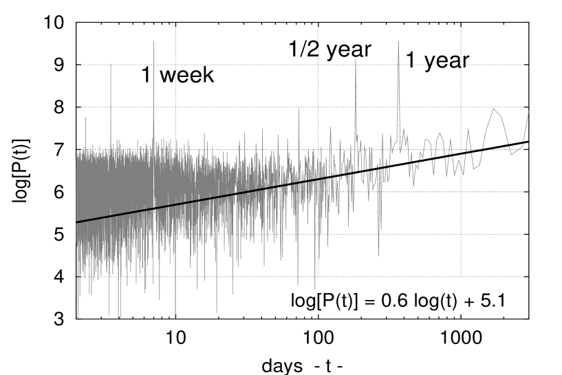
FIG. 2.: Spectral analysis of the births to teenagers as a function of the time period, measured in days. From the right to the left the periods revealed by this analysis are: 3.5 days, 7 days, 73 days, 183 days, 365 days. The background noise exhibits a scaling behavior similar to that of a fractional Gaussian noise at least for a large period of time, from one or two months to 8 years. The straight line corresponds to the scaling condition with $\beta=2H-1=0.60$ assuming $H=\delta=0.80$ measured in Sec. 5.

FIG. 3.: WMA of the births to teenagers. The figures show the smooth curves $S_{5}$, $S_{6}$, $S_{7}$, $S_{8}$. These curves smooth all fluctuations with a period shorter than 64, 128, 256 and 512 days, respectively.

FIG. 4.: WMA of the births to teenagers. The figures show the detail curves $D_{2}$, $D_{4}$, $D_{7}$ and $D_{8}$. These curves contain fluctuations with a period within the range of [4:8], [16:32], [128:256] and [256:512] days, respectively.

FIG. 5.: WMA of the births to teenagers. [a] The first picture shows the smooth curves $S_{4}$ (full line) and $S_{9}$ (dashed line) that smooth all fluctuations with period shorter than 32 and 1024 days, respectively. [b] The second picture shows the original data with the smooth curve $S_{9}$ detrended from them. [c] The third figure shows the smooth curve $S_{4}$, with the smooth curve $S_{9}$ detrended from it.

FIG. 6.: Daily birth rate through the months of the year. These values are obtained from the 36 yearly cycles of Fig. 6, obtained by detrending the smooth curve $S_{9}$ from the original data. For each day of the year we evaluate the mean value of the birth rate over the 36 years of the 1964-1999 time period. The lowest rates occur in April and May, and the highest in August and September. There are deep spikes in the correspondence of holidays: first days of January, 4th of July, first week of September and 25th-26th of December.

FIG. 7.: Daily conception rate through the months of the year. The values are obtained from the smooth curve $S_{4}$, with the smooth curve $S_{9}$ detrended from it (Fig. 7). For each day of the year we evaluate the mean value over the 36 years of the 1964-1999 time period. The conception day is estimated to occur 38 weeks before the delivery. The lowest rate is in July and August, the highest in November and December. There is a conception rate increase during the holidays: Spring break in March, Thanksgiving in November and Christmas in December. A fast growth of the conception rate occurs in September and October.

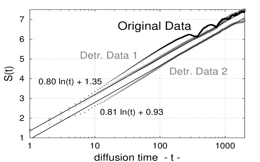
FIG. 8.: DEA of the Births to teenagers of the original data (black curve), of the data detrended of the details $D_{8}$ and $D_{7}$ that correspond to the annual and one half annual periodicity (gray circle curve) and of the data detrended (dotted line) of the details $D_{8}$ and $D_{7}$ plus the linear fit $y=a+b(t-1964)$ discussed in Sec. 2 (gray star curve). The slope of the straight line, $\delta=0.80\pm 0.02$, is the scaling coefficient of the background noise according to Eq. (10).

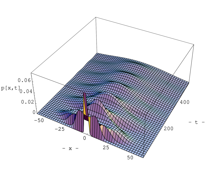
FIG. 9.: The figure shows the pdf $p(x,t)$ given by Eq. (22). This pdf is the convolution of the Gaussian diffusion pdf $p_{s}(x,t)$ of Eq. (23) and of the deterministic pdf $p_{d}(x,t)$ of Eq. (25). The period of the deterministic component is $T=100$ and the amplitude is $A=1$. By increasing the diffusion time $t$ the effect of the deterministic component becomes weaker and weaker and the Gaussian component prevails in accordance to the Central Limit Theorem.

FIG. 10.: The figure shows the convoluted pdf $p(x,t)$ given by Eq. (22) and the Gaussian pdf $p_{s}(x,t)$ of Eq. (23) (upper curve) at $x=0$. The period of the deterministic component is $T=100$ and the amplitude is $A=1$. By increasing the diffusion time $t$ the two curves converge in accordance to the Central Limit Theorem.

FIG. 11.: Difference $k(t)$ against the diffusion time $t$. According to the theory, $k(t)\simeq t^{-1.5}$ for large $t$.

FIG. 12.: DEA of the artificial dataset $\{\zeta_{i}\}$, Eq. (18), (solid line) and of the Gaussian artificial dataset $\{\eta_{i}\}$ (dashed line). The dashed curve coincides with a straight line with the slope $\delta=0.5$. The constant $S_{d}(1)$ is the value of the entropy of the artificial dataset $\{\eta_{i}\}$ at the first step of diffusion.

FIG. 13.: [a] Time series of an artificial fractional Gaussian noise with H=0.80 and its smooth curve obtained with a moving average of period $T=300$ (generic units). [b] Diffusion entropy analysis of the original fractal noise (upper curve) and of the residual noise (lower curve) obtained by detrending the original noise of the smooth component. The figure shows that the smoothing detrending procedure disrupts completely the scaling and fractal properties of the original signal.

FIG. 14.: MDEA of the Births to teenagers. From top to down, the curves are the DEA of the original data, and of the residuals $R_{8}$, …, $R_{3}$. The straight line is $f_{DE}(t)=0.5\ln(t)$ that corresponds to the Gaussian diffusion. Above the straight line there is the persistent region and below the straight line there is the antipersistent region.

	S(1)	Ssat	Ssat	period
		rel-val	abs-val	days
data	1.45	Min : Max	Min : Max
$R_{8}$	1.22	2.00 : 3.50	3.22 : 4.72	365
$R_{7}$	1.19	1.60 : 2.60	2.79 : 3.79	183
$R_{6}$	1.18	1.00 : 1.30	2.18 : 2.48	75
$R_{5}$	1.17	0.65 : 0.85	1.82 : 2.02	7 & 45
$R_{4}$	1.15	0.30 : 0.60	1.45 : 1.75	7 & 21
$R_{3}$	1.03	0.00 : 0.44	1.03 : 1.47	7

TABLE I.: Summary of the information contained in Fig. 14. The first column reports the values of the entropy at the first step of diffusion, S(1), for the original data and their rests $R_{j}$ for $j=2,...,8$. The second and third columns report the relative and the absolute values of the range of the height of the horizontal lines that measure the information or entropy that corresponds to each wavelet scale. The absolute values of the entropy of the third column are obtained by summing the values of column 1 and 2. The last column reports the main periodicity present in each rest $R_{j}$. The rests $R_{8}$ and $R_{7}$ are dominated by the annual periodicity and its harmonic. The rests $R_{5}$, $R_{4}$, $R_{3}$ are dominated by the strong weekly periodicity. The values are compatible with those given by the spectral analysis of Fig. 2.

REFERENCES

- [1] P. Grigolini, D. Leddon, N. Scafetta, Phys. Rev. E 65, 046203 (2002).
- [2] N. Scafetta, P. Hamilton and P. Grigolini, Fractals, 9, 193-208 (2001).
- [3] N. Scafetta and P. Grigolini, Phys. Rev. E 66, 036130 (2002).
- [4] P. Allegrini, V. Benci, P. Grigolini, P. Hamilton, M. Ignaccolo, G. Menconi, L. Palatella, G. Raffaelli, N. Scafetta, M. Virgilio, J. Jang, Chaos, Solitons & Fractals 15 (3), 517-535 (2003).
- [5] Lam, David A.; Miron, Jeffrey A. Silver Spring, Maryland. Demography, Vol. 33, No. 3, 291-305, Aug (1996).
- [6] D. B. Percival and A. T. Walden, Wavelet Methods for Time Series Analysis, Cambridge University Press, Cambridge (2000).
- [7] Texas Department of Health, Bureau of Vital Statistics, Statistical Services Division (1999). Texas Vital Statistics, 1999, p. 294.
- [8] B.J. West, P. Hamilton and D.J. West, Fractals 7, 113-122 (1999).
- [9] N. Gleicher, L. Buttino, V. Elkayam, M. Evans, R. Galbraith, S. Gall and B. Sibai, Principles and practice of medical therapy in pregnancy, third edition, McGraw-Hill (1998).
- [10] S. G. Gabbe, J. R. Niebyl, J. L. Simpson and M. Senkarik, Obstetrics, normal and problem pregnancies, fourth edition, Churchill Livingstone, (2001).
- [11] N. Scafetta, P. Grigolini, P. Hamilton and B. J. West, in Nonextensive Entropy: Interdisciplinary Applications, Editors M. Gell-Mann and C. Tsallis, Proceedings Volume in the Sante Fe Institute Studies in the Science of Complexity, Oxford University Press (2004).
- [12] B.B. Mandelbrot, The Fractal Geometry of Nature, (Freeman, New York, 1983).
- [13] H.E. Stanley, L.A.N. Amaral, P. Gopikrishnan, P. Ch. Ivanov, T.H. Keitt, V. Plerou, Physica A 281 60-68 (2000).
- [14] C. K. Peng, S. V. Buldyrev, S. Havlin, M. Simons, H. E. Stanley, and A. L. Goldberger, Phys. Rev, E 49, 1685-1689 (1994).
- [15] N. Scafetta, V. Latora, P. Grigolini, Phys. Rev. E 66, 031906 (2002).
- [16] Committee on Adolescence of the American Academy of Pediatrics. Adolescent Pregnancy-Current Trends and Issues: 1998 (RE 9828). Pediatrics. Vol. 103, No 2 pp 516-520 (1999).
- [17] D.A. Savitz, C.A. Blackmore, J.M. Thorp, Epidemiologic Characteristics of Preterm Delivery: etiologic heterogeneity, Etiologic heterogeneity. Am J Obstet Gynecol 164 467-71 (1991).