Quasistatic Scale-free Networks

Abstract

A network is formed using the $N$ sites of an one-dimensional lattice in the shape of a ring as nodes and each node with the initial degree $k_{in}=2$. $N$ links are then introduced to this network, each link starts from a distinct node, the other end being connected to any other node with degree $k$ randomly selected with an attachment probability proportional to $k^{\alpha}$. Tuning the control parameter $\alpha$ we observe a transition where the average degree of the largest node $\langle k_{m}(\alpha,N)\rangle$ changes its variation from $N^{0}$ to $N$ at a specific transition point of $\alpha_{c}$. The network is scale-free i.e., the nodal degree distribution has a power law decay for $\alpha\geq\alpha_{c}$.

The nodal degree distribution function of a scale-free network (SFN) has a power law tail barabasi . Empirical data obtained for several social, biological and computational networks have confirmed existence of such probability distributions decaying as power laws albert ; neural ; collab . For example the World-wide web web which is a network of web pages and the hyper-links among various pages and the Internet network Faloutsos of routers or autonomous systems follow power laws as: $P(k)\sim k^{-\gamma}$. The exponent $\gamma$ varies between 2 and 3 for these networks.

Networks are classified here as ‘growing’, ‘quasistatic’ and ‘static’. In a growing network (GN) the nodes are introduced in the network one after another. After introducing the node a link is introduced connecting this node to one of its previous nodes. Therefore, in a GN both the numbers of nodes as well as links grow with time. In contrast, in the case of a quasistatic network (QN) a fixed number $N$ of nodes are present at the initial stage. $N$ Links are then introduced one after another between pairs of nodes using some specific probability distribution. Therefore in a QN, the number of nodes in the network is fixed but the number of links grow with time. Finally, in a static network (SN) both the number of nodes as well as the number of links remain fixed and donot grow with time.

Barabási and Albert (BA) proposed barabasi a simple model for a growing SFN that has the following two essential ingredients, namely: (i) A network grows from an initial set of $m_{o}$ nodes with $m<m_{o}$ links among them. Further, at every time step a new node is introduced and is randomly connected to $m$ previous nodes. (ii) Any of these $m$ links of the new node introduced at time $t$ connects a previous node $i$ with an attachment probability $\pi_{i}(t)$ which is linearly proportional to the degree $k_{i}(t)$ of the $i$-th node at time $t$: $\pi^{BA}_{i}(t)\sim k_{i}(t)$. For BA model $\gamma=3$ albert .

Figure 1: A quasistatic scale-free network with 128 nodes placed on a circular ring so that the initial degree $k_{init}$ of each node is equal to 2. Nodes are then selected one after another without repetition and are randomly linked to other nodes with an attachment probability proportional to $k^{\alpha}$. In this picture $\alpha=2.6$ is used and a large degree node is visible.

The second criterion reflects the phenomenon of ‘rich gets richer’ i.e., a node with a large degree attracts more nodes to get linked. Krapivsky et. al. showed that this linear dependence is a necessary condition and any other non-linear dependence on the degree destroys the scale-free behaviour i.e., the power law variation of the degree distribution redner . Indeed, if in general the degree dependence has a variation with the $\alpha$-th power of the degree, it has been shown that the scale-free nature of the BA model network exists only for $\alpha=1$ and for no other value of it, smaller or larger.

Several other interesting networks are also studied. Erdös and Rényi studied long ago random graphs of $N$ nodes where links are introduced with probability $p$ between arbitrary pairs of randomly selected nodes random . A largest component of such a network connecting nodes of the order of $N$ appears at a particular value of $p_{c}=1/N$. Very recently SFNs are studied on Euclidean spaces where the BA attachment probability is modified by a link length $\ell$ dependent factor Manna_Sen ; euclid ; jost ; yook2 . Load distribution in Scale-free networks has also been studied Goh .

In this paper we ask the question if the growing condition of the BA model is really a necessity to achieve a scale-free network. We will see below that it is not, a suitable choice of the attachment probability in a quasistatic network may result a power law decay for the degree distribution as well. We call our model as the Quasitatic Scale-free Network (QSFN). Recently Doye has shown that the network topology of a potential energy landscape is a static scale-free network Doye . Assigning a quenched intrinsic fitness to every node and using the attachment probabilities depending on the fitnesses it is also possible to get SFNs without growth and preferential attachments Caldarelli . A steady state model for scale-free graphs has also been proposed Eppstein .

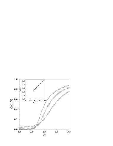
Figure 2: The variation of the order parameter $\phi(\alpha,N)$ which is the average degree of the largest node divided by $N$ with $\alpha$ for three different network sizes $N=2^{8}$ (circle), $2^{10}$ (square) and $2^{12}$ (triangle). The inset shows the plot of the threshold values $\alpha_{c}(N)$ with $N^{-0.2}$ for seven different $N$ values from $2^{7}$ to $2^{13}$ increasing by a factor of 2 at each step.

Our quasistatic model starts with an one-dimensional regular lattice in the form of a circular ring as in the Watts and Strogatz’s Small-world Network WS . The lattice has $N$ nodes serially marked from $i$=1 to $N$ and $N$ links between successive pairs of nodes with periodic boundary condition. Each node is therefore connected to only two of its nearest neighbours situated on the opposite sides and the degree $k_{i}$ for each node $i$ is exactly 2 to begin with. We add to this system another $N$ distinct links in total, such that a new link starts from each node. A $t$-th link is added at time $t$ and one end of it is attached to the $t$-th node, the other end of the link is connected to a node $j$ with degree $k_{j}(t)$ selected randomly from the rest of the $N-1$ nodes of the system using the following attachment probability:

$$\pi_{j}(t)\sim k_{j}^{\alpha}(t)$$ (1)

where $\alpha$ is a continuously tunable parameter. Therefore when the network is complete no node is left with degree 2.

At this point we would like to clearly distinguish between our QSFN and the model B modelB . Model B also starts with a collection of $N$ nodes but no links, so that the initial degree of each node is strictly zero and the graph has $N$ components each with only one node. At each time step a node $i$ is selected randomly with uniform probability and is connected to another node $j$ with a probability $\pi_{j}(t)\sim k_{j}(t)$. This implies that isolated nodes are being linked one by one to a single connected component of the graph. For this component, both the number of nodes as well as the links grow with time and therefore model B is clearly a growing network. This is in contrast to our QSFN model where the initial network is a $N$ node connected graph which grows by adding further links but not the nodes any more.

Figure 3: The local derivative of the order parameter $d\phi(\alpha,N)/d\alpha$ has been plotted with $\alpha$ for 7 different $N$ values starting from $2^{7}$ and increasing by a factor of 2. Scaling of the derivative is done in the inset for $N=2^{8},2^{10}$ and $2^{12}$ by plotting $[d\phi(\alpha,N)/d\alpha]N^{-0.21}$ vs. $[\alpha-\alpha_{c}(N)]N^{0.18}$.

In the case of $\alpha=0$ in QSFN, all nodes have equal probabilities to get connected by a new link and this is the random network model random for which the degree distribution is the Poisson distribution albert . For $\alpha>0$, a node with larger degree has a higher probability to get connected by links. The case of $\alpha=1$ corresponds to the similar attachment probability as in the BA model of SFN. Our simulation results show that the degree distribution in this case has an exponentially decaying form: $P(k)\sim\exp(-ak)$ with $a\approx 1.08$. On continuously increasing $\alpha$ further larger degree nodes become more probable and we see that the degree distribution decays less sharply and changes to a stretched exponential form as: $P(k)\sim\exp[-k^{\chi(\alpha)})]$. The exponent $\chi(\alpha)$ decreases continuously from its value 1 at $\alpha=1$ to $\chi\approx 0.3$ at $\alpha=1.75$.

On increasing the parameter $\alpha$ further the system makes a transition to a different behaviour where a single node having the maximum degree $k_{m}$ connects to a finite fraction of the $N$ nodes. However this transition takes place at a specific value $\alpha_{c}$ of $\alpha$ so that the degree distribution has a power law tail and therefore the network is scale-free for all $\alpha\geq\alpha_{c}$.

Naturally the control parameter in this model is $\alpha$ where as like the phenomenon of percolation, an order parameter in this problem may be the average degree of the largest node $\phi(\alpha,N)=\langle k_{m}(\alpha,N)\rangle/N$. We monitor the variation of $\phi(\alpha,N)$ with $\alpha$ and plot them in Fig. 2 for networks of three different sizes $N=2^{8},2^{10}$ and $2^{12}$. A sharp increase in the order parameter is observed around $\alpha=2$, again the sharpness of the curves increases with $N$. The first derivative $d\phi(\alpha,N)/d\alpha$ of the order parameter is plotted in Fig. 3 for seven different network sizes. Every curve has a peak at some $N$ dependent value of $\alpha_{c}(N)$ where $\phi(\alpha,N)$ increases at the fastest rate. For locating the precise value of $\alpha_{c}(\infty)$ where this transition is taking place for an infinitely large network, we plot $\alpha_{c}(N)$ values as a function of $N^{-1/\nu}$ in the inset of Fig. 2. Using a trial value of $\nu=5$ we could get all seven points on a straight line and on extrapolating to the $N\rightarrow\infty$ limit we get $\alpha_{c}(\infty)=1.85\pm 0.10$.

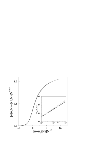
Figure 4: Scaling of the order parameter: $[\phi(\alpha,N)-\phi(1,N)]N^{0.025}$ is plotted with $[\alpha-\alpha_{c}(N)]N^{1/3}$ for the data collapse. The inset shows that average degree of the largest node $\langle k_{m}(\alpha,N)\rangle$ varies as $N^{\mu}$ at the transition point $\alpha_{c}$ where we obtained $\mu=0.91\pm 0.04$. The dotted line, having a slope unity, is given to compare with the data.

All the first derivative curves are suitably scaled in the inset of Fig. 3 and the data are collapsed. Each curve is first shifted by an amount $\alpha_{c}(N)$. Then the abscissa is scaled by $N^{0.18}$ and the ordinate is scaled by $N^{-0.21}$ and we get a nice collapse of three curves of sizes $N=2^{8},2^{10}$ and $2^{12}$. This analysis implies that the order parameter curves in Fig. 2 become progressively sharper as the network size $N$ gradually increases and $\phi(\alpha,N)$ increases very rapidly at $\alpha_{c}(\infty)$. This variation is very similar to the variation of the order parameter (the fraction of mass in the largest cluster) in the percolation phenomena.

The scaling of the order parameter $\phi(\alpha,N)$ is shown in Fig. 4. Asymptotically as $N\rightarrow\infty$ the $\phi(\alpha,N)\rightarrow 0$ for $\alpha<\alpha_{c}$ but for finite $N$ we subtract the $\phi(1,N)$ from $\phi(\alpha,N)$ and try to scale only the difference. We assume the following scaling behaviour:

$$[\phi(\alpha,N)-\phi(1,N)]N^{\beta/\nu}={\cal F}[(\alpha-\alpha_{c})N^{1/\nu}]$$ (2)

where the scaling function ${\cal F}(x)\rightarrow x^{\beta}$ for $x<<1$. From Fig. 4 we get $\nu=3$ and $\beta=0.075$. This value of $\nu$ is not very consistent with its value 5 obtained in the inset of Fig. 2. We believe this difference is due to finite size of our simulations.

The dependence of the average degree $\langle k_{m}(\alpha_{c},N)\rangle$ of the largest node right at the transition point $\alpha=\alpha_{c}$ is also studied and plotted in the inset of Fig. 4 on a double logarithmic scale. Assuming a power law dependence on the network size with an exponent $\mu$ as $\langle k_{m}(\alpha_{c},N)\rangle\sim N^{\mu}$ the plot gives a value of $\mu=0.91\pm 0.04$. Here $\mu$ is an exponent similar to the fractal dimension of the infinite incipient percolation clusters at the percolation threshold.

Figure 5: Scaled degree distributions at the transition points $\alpha_{c}(N)$ for different network sizes have been plotted. Data collapse is obtained for large $k$ values when $P(k,\alpha_{c},N)N^{\eta}$ has been plotted with $k/N^{\xi}$ with $\eta=3$ and $\xi=1$. This gives the degree distribution exponent $\gamma=\eta/\xi=3$.

Finally the degree distribution $P(k,\alpha_{c}(N),N)$ is calculated for different network sizes $N$ at their transition points $\alpha_{c}(N)$. In these calculations we have not counted the maximum degree node similar to what is usually done to estimate the cluster size distribution at the percolation threshold. Except for very small $k$ values all distribution curves have straight portions on double logarithmic plots and the region over which nearly constant slopes are observed, increases with increasing $N$. The fluctuating data is suitably binned: for each $k$ value the data is averaged over the bin from $k$ to $2k-1$ and is plotted at $[k(2k-1)]^{1/2}$. We assume a scaling form like:

$$P(k,\alpha_{c}(N),N)N^{\eta}\sim{\cal G}(k/N^{\xi})$$ (3)

where ${\cal G}(x)$ is expected to be an universal scaling function such that ${\cal G}(x)\rightarrow x^{-\gamma}$ for $x<<1$ so that $\gamma=\eta/\xi$. The scaling plot is shown in Fig. 5 where we get $\eta=3$ and $\xi=1$ giving $\gamma=3$ as in the BA model of SFN. This is a very interesting result that even on a static network with a suitable attachment probability $k^{\alpha}$ with a non-trivial value of $\alpha$ one gets a scale-free degree distribution for the network, the distribution being the same as the BA model of SFN.

What happens when $\alpha>\alpha_{c}$? Our observation is that degree distribution is still a power law but the exponent $\gamma$ is now $\alpha$ dependent. In the range of $\alpha\geq 3$, the degree exponent $\gamma$ is approximately equal to $\alpha$ whereas for $\alpha_{c}\leq\alpha\leq 3$, $\gamma(\alpha)\approx 3$.

We also have tried a more stochastic version of this model where to add a link, we select in parallel two nodes arbitrarily from the whole set of $N$ nodes using the attachment probability in Eqn. (1). If these two nodes are not the same node, we connect them. This is also a QSFN but the difference here is both the nodes of each link are selected randomly where as in the QSFN described above only one node is selected randomly and the other node is selected systematically one after another from the set of nodes. Our numerical studies indicate that behaviours of both versions are very similar.

Another variation of our model has been studied with initial degrees of all nodes as $k_{in}=1$ which corresponds to a situation where alternate pairs of nodes on an one-dimensional ring shaped lattice are linked. Again we numerically observe that the $\alpha_{c}=1.67\pm 0.10$ and $\gamma(\alpha_{c})\approx 2.5$ for this model.

To summarize, we have studied a quasistatic scale-free network (QSFN) where we have a collection of $N$ nodes initially present, each node is having $k_{in}$ initial degree. A system of $N$ links are then introduced, one corresponding to each node. That means we systematically attach the one end of each link to one node, the other end of the link is probabilistically attached to any other node of degree $k$ with a probability proportional to $k^{\alpha}$. Our numerical study indicates that there exists a transition point $\alpha_{c}$ beyond which the resulting network has a scale-free structure so that the degree distribution has a power law tail for $\alpha\geq\alpha_{c}$.

We thankfully acknowledge P. Sen, D. Stauffer and D. Dhar for critical reading of the manuscript and many useful comments and also A.-L. Barabási for helpful suggestions. GM gratefully acknowledges the hospitality at the S. N. Bose National Centre for basic sciences.

Correspondence to: manna@boson.bose.res.in

References

- (1) A.-L. Barabási and R. Albert, Science, 286, 509 (1999).
- (2) R. Albert and A.-L. Barabási, Rev. Mod. Phys. 74, 47 (2002).
- (3) J. J. Hopfield and A. V. M. Herz, Proc. Natl. Acad. Sci. USA, 92, 6655 (1995).
- (4) M. E. J. Newman, Proc. Nat. Acad. Sci. USA, 98, 404 (2001); arXiv:cond-mat/0011155.
- (5) S. Lawrence and C. L. Giles, Science, 280, 98 (1998); Nature, 400, 107 (1999), R. Albert, H. Jeong and A.-L. Barabási, Nature, 401, 130 (1999).
- (6) M. Faloutsos, P. Faloutsos and C. Faloutsos, Proc. ACM SIGCOMM, Comput. Commun. Rev., 29, 251 (1999).
- (7) P. L. Krapivsky, G. J. Rodgers and S. Redner, Phys. Rev. Lett. 86, 5401 (2001); P. L. Krapivsky and S. Redner, Phys. Rev. E, 63, 066123 (2001).
- (8) P. Erdös and A. Rényi, Publ. Math. Debrecen, 6, 290 (1959).
- (9) S. S. Manna and P. Sen, arXiv:cond-mat/0203216.
- (10) S. Jespersen and A. Blumen, Phys. Rev. E 62, 6270 (2000); J. Kleinberg, Nature 406, 845 (2000); S. N. Dorogovtsev, J.F.F. Mendes and A.N.Samukhin, arXiv:cond-mat/0206467.
- (11) J. Jost and M. P. Joy, arXiv:cond-mat/0202343.
- (12) S. H. Yook, H. Jeong, A.-L. Barabási and Y. Tu, Phys. Rev. Lett. 86, 5835 (2001).
- (13) K.-I. Goh, B. Khang and D. Kim, Phys. Rev. Lett. 87, 278701 (2001).
- (14) J. P. K. Doye, Phys. Rev. Lett. 23, 238701 (2002).
- (15) G. Caldarelli, A. Capocci, P. De Los Rios and M. A. Muñoz, arXiv:cond-mat/0207366.
- (16) D. Eppstein and J. Wang, arXiv:cs.DM/0204001.
- (17) D. J. Watts and S. H. Strogatz, Nature, 393, 440 1998; D. J. Watts, Small Worlds: The Dynamics of Networks Between order and Randomness, (Princeton 1999).
- (18) A.-L. Barabási, R. Albert and H. Jeong, Physica A, 272, 173 (1999).