Multi-Moments Method for Portfolio Management:
Generalized Capital Asset Pricing Model
in Homogeneous and Heterogeneous markets

Abstract

We introduce a new set of consistent measures of risks, in terms of the semi-invariants of pdf’s, such that the centered moments and the cumulants of the portfolio distribution of returns that put more emphasis on the tail the distributions. We derive generalized efficient frontiers, based on these novel measures of risks and present the generalized CAPM, both in the cases of homogeneous and heterogeneous markets. Then, using a family of modified Weibull distributions, encompassing both sub-exponentials and super-exponentials, to parameterize the marginal distributions of asset returns and their natural multivariate generalizations, we offer exact formulas for the moments and cumulants of the distribution of returns of a portfolio made of an arbitrary composition of these assets. Using combinatorial and hypergeometric functions, we are in particular able to extend previous results to the case where the exponents of the Weibull distributions are different from asset to asset and in the presence of dependence between assets. In this parameterization, we treat in details the problem of risk minimization using the cumulants as measures of risks for a portfolio made of two assets and compare the theoretical predictions with direct empirical data. Our extended formulas enable us to determine analytically the conditions under which it is possible to “have your cake and eat it too”, i.e., to construct a portfolio with both larger return and smaller “large risks”.

1 Introduction

The Capital Asset Pricing Model (CAPM) is still the most widely used approach to relative asset evaluation, although its empirical roots are been found weaker and weaker in recent years. This asset valuation model describing the relationship between expected risk and expected return for marketable assets is strongly entangled with the Mean-Variance Portfolio Model. Indeed both of them fundamentally rely on the description of the probability distribution function (pdf) of asset returns in terms of Gaussian functions. The Mean-Variance description is thus at the basis of Markovitz’s portfolio theory [Markovitz (1959)] and of the CAPM (see for instance [Merton (1990)]).

Otherwise, the determination of the risks and returns associated with a given portfolio constituted of $N$ assets is completely embedded in the knowledge of their multivariate distribution of returns. Indeed, the dependence between random variables is completely described by their joint distribution. This remark entails the two major problems of portfolio theory: 1) determine the multivariate distribution function of asset returns; 2) derive from it useful measures of portfolio risks and use them to analyze and optimize portfolios.

The variance (or volatility) of portfolio returns provides the simplest way to quantify its fluctuations and is at the fundation of the [Markovitz (1959)]’s portfolio selection theory. Nonetheless, the variance of a portfolio offers only a limited quantification of incurred risks (in terms of fluctuations), as the empirical distributions of returns have “fat tails” [Lux (1996), Gopikrishnan et al. (1998), among many others] and the dependences between assets are only imperfectly accounted for by the covariance matrix [Litterman and Winkelmann (1998)]. It is thus essential to extend portfolio theory and the CAPM to tackle these empirical facts.

The Value-at-Risk [Jorion (1997)] and many other measures of risks [Artzner et al. (1997), Sornette (1998), Artzner et al. (1999), Bouchaud et al. (1998), Sornette et al. (2000b)] have then been developed to account for the larger moves allowed by non-Gaussian distributions and non-linear correlations but they mainly allow for the assessment of down-side risks. Here, we consider both-side risk and define general measures of fluctuations. It is the first goal of this article. Indeed, considering the minimum set of properties a fluctuation measure must fulfil, we characterize these measures. In particular, we show that any absolute central moments and some cumulants satisfy these requirement as well as do any combination of these quantities. Moreover, the weights involved in these combinations can be interpreted in terms of the portfolio manager’s aversion against large fluctuations.

Once the definition of the fluctuation measures have been set, it is possible to classify the assets and portfolios using for instance a risk adjustment method [Sharpe (1994), Dowd (2000)] and to develop a portfolio selection and optimization approach. It is the second goal of this article.

Then a new model of market equilibrium can be derived, which generalizes the usual Capital Asset Pricing Model (CAPM). This is the third goal of our paper. This improvement is necessary since, although the use of the CAPM is still widely spread, its empirical justification has been found less and less convincing in the past years [Lim (1989), Harvey and Siddique (2000)].

The last goal of this article is to present an efficient parametric method allowing for the estimation of the centered moments and cumulants, based upon a maximum entropy principle. This parameterization of the problem is necessary in order to obtain accurate estimates of the high order moment-based quantities involved the portfolio optimization problem with our generalized measures of fluctuations.

The paper is organized as follows.

Section 2 presents a new set of consistent measures of risks, in terms of the semi-invariants of pdf’s, such as the centered moments and the cumulants of the portfolio distribution of returns, for example.

Section 3 derives the generalized efficient frontiers, based on these novel measures of risks. Both cases with and without risk-free asset are analyzed.

Section 4 offers a generalization of the Sharpe ratio and thus provides new tools to classify assets with respect to their risk adjusted performance. In particular, we show that this classification may depend on the choosen risk measure.

Section 5 presents the generalized CAPM based on these new measures of risks, both in the cases of homogeneous and heterogeneous agents.

Section 6 introduces a novel general parameterization of the multivariate distribution of returns based on two steps: (i) the projection of the empirical marginal distributions onto Gaussian laws via nonlinear mappings; (ii) the use of an entropy maximization to construct the corresponding most parsimonious representation of the multivariate distribution.

Section 7 offers a specific parameterization of marginal distributions in terms of so-called modified Weibull distributions, which are essentially exponential of minus a power law. Notwithstanding their possible fat-tail nature, all their moments and cumulants are finite and can be calculated. We present empirical calibration of the two key parameters of the modified Weibull distribution, namely the exponent $c$ and the characteristic scale $\chi$.

Section 8 provides the analytical expressions of the cumulants of the distribution of portfolio returns for the parameterization of marginal distributions in terms of so-called modified Weibull distributions, introduced in section 6. Empirical tests comparing the direct numerical evaluation of the cumulants of financial time series to the values predicted from our analytical formulas find a good consistency.

Section 9 uses these two sets of results to illustrate how portfolio optimization works in this context. The main novel result is an analytical understanding of the conditions under which it is possible to simultaneously increase the portfolio return and decreases its large risks quantified by large-order cumulants. It thus appears that the multidimensional nature of risks allows one to break the stalemate of no better return without more risks, for some special kind of rational agents.

Section 10 concludes.

Before proceeding with the presentation of our results, we set the notations to derive the basic problem addressed in this paper, namely to study the distribution of the sum of weighted random variables with arbitrary marginal distributions and dependence. Consider a portfolio with $n_{i}$ shares of asset $i$ of price $p_{i}(0)$ at time $t=0$ whose initial wealth is

$$W(0)=\sum_{i=1}^{N}n_{i}p_{i}(0)~{}.$$ (1)

A time $\tau$ later, the wealth has become $W(\tau)=\sum_{i=1}^{N}n_{i}p_{i}(\tau)$ and the wealth variation is

$$\delta_{\tau}W\equiv W(\tau)-W(0)=\sum_{i=1}^{N}n_{i}p_{i}(0){{p_{i}(\tau)-p_{i}(0)}\over p_{i}(0)}=W(0)~{}\sum_{i=1}^{N}w_{i}r_{i}(t,\tau),$$ (2)

where

$$w_{i}={n_{i}p_{i}(0)\over\sum_{j=1}^{N}n_{j}p_{j}(0)}~{}$$ (3)

is the fraction in capital invested in the $i$th asset at time $0$ and the return $r_{i}(t,\tau)$ between time $t-\tau$ and $t$ of asset $i$ is defined as:

$$r_{i}(t,\tau)={p_{i}(t)-p_{i}(t-\tau)\over p_{i}(t-\tau)}~{}.$$ (4)

Using the definition (4), this justifies us to write the return $S_{\tau}$ of the portfolio over a time interval $\tau$ as the weighted sum of the returns $r_{i}(\tau)$ of the assets $i=1,...,N$ over the time interval $\tau$

$$S_{\tau}={\delta_{\tau}W\over W(0)}=\sum_{i=1}^{N}w_{i}~{}r_{i}(\tau)~{}.$$ (5)

In the sequel, we shall thus consider asset returns as the fundamental variables (denoted $x_{i}$ or $X_{i}$ in the sequel) and study their aggregation properties, namely how the distribution of portfolio return equal to their weighted sum derives for their multivariable distribution. We shall consider a single time scale $\tau$ which can be chosen arbitrarily, say equal to one day. We shall thus drop the dependence on $\tau$, understanding implicitely that all our results hold for returns estimated over the time step $\tau$.

2 Measuring large risks of a portfolio

The question on how to assess risk is recurrent in finance (and in many other fields) and has not yet received a general solution. Since the middle of the twentieth century, several paths have been explored. The pioneering work by [Von Neuman and Morgenstern (1947)] has given birth to the mathematical definition of the expected utility function which provides interesting insights on the behavior of a rational economic agent and formalized the concept of risk aversion. Based upon the properties of the utility function, [Rothschild and Stiglitz (1970)] and [Rothschild and Stiglitz (1971)] have attempted to define the notion of increasing risks. But, as revealed by [Allais (1953), Allais (1990)], empiric investigations has proven that the postulates chosen by [Von Neuman and Morgenstern (1947)] are actually often violated. Many generalizations have been proposed for curing the so-called Allais’ Paradox, but up to now, no generally accepted procedure has been found in this way.

Recently, a theory due to [Artzner et al. (1997), Artzner et al. (1999)] and its generalization by
[Föllmer and Schied(2002a), Föllmer and Schied(2002b)], have appeared. Based on a series of postulates that are quite natural, this theory allows one to build coherent (convex) measures of risks. In fact, this theory seems well-adapted to the assessment of the needed economic capital, that is, of the fraction of capital a company must keep as risk-free assets in order to face its commitments and thus avoid ruin. However, for the purpose of quantifying the fluctuations of the asset returns and of developing a theory of portfolios, this approach does not seem to be operational. Here, we shall rather revisit [Markovitz (1959)]’s approach to investigate how its extension to higher-order moments or cumulants, and any combination of these quantities, can be used operationally to account for large risks.

2.1 Why do higher moments allow to assess larger risks?

In principle, the complete description of the fluctuations of an asset at a given time scale is given by the knowledge of the probability distribution function (pdf) of its returns. The pdf encompasses all the risk dimensions associated with this asset. Unfortunately, it is impossible to classify or order the risks described by the entire pdf, except in special cases where the concept of stochastic dominance applies. Therefore, the whole pdf can not provide an adequate measure of risk, embodied by a single variable. In order to perform a selection among a basket of assets and construct optimal portfolios, one needs measures given as real numbers, not functions, which can be ordered according to the natural ordering of real numbers on the line.

In this vein, [Markovitz (1959)] has proposed to summarize the risk of an asset by the variance of its pdf of returns (or equivalently by the corresponding standard deviation). It is clear that this description of risks is fully satisfying only for assets with Gaussian pdf’s. In any other case, the variance generally provides a very poor estimate of the real risk. Indeed, it is a well-established empirical fact that the pdf’s of asset returns has fat tails [Lux (1996), Pagan (1996), Gopikrishnan et al. (1998)], so that the Gaussian approximation underestimates significantly the large prices movements frequently observed on stock markets. Consequently, the variance can not be taken as a suitable measure of risks, since it only accounts for the smallest contributions to the fluctuations of the assets returns.

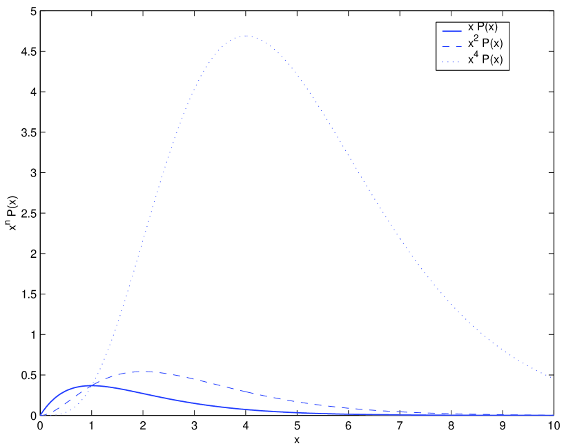
Figure 1: This figure represents the function $x^{n}\cdot e^{-x}$ for $n=1,2$ and $4$. It shows the typycal size of the fluctuations involved in the moment of order $n$.

The variance of the return $X$ of an asset involves its second moment ${\rm E}[X^{2}]$ and, more precisely, is equal to its second centered moment (or moment about the mean) ${\rm E}\left[\left(X-{\rm E}[X]\right)^{2}\right]$. Thus, the weight of a given fluctuation $X$ entering in the definition of the variance of the returns is proportional to its square. Due to the decay of the pdf of $X$ for large $X$ bounded from above by $\sim 1/|X|^{1+\alpha}$ with $\alpha>2$, the largest fluctuations do not contribute significantly to this expectation. To increase their contributions, and in this way to account for the largest fluctuations, it is natural to invoke higher order moments of order $n>2$. The large $n$ is, the larger is the contribution of the rare and large returns in the tail of the pdf. This phenomenon is demonstrated in figure 1, where we can observe the evolution of the quantity $x^{n}\cdot P(x)$ for $n=1,2$ and $4$, where $P(x)$, in this example, is the standard exponential distribution $e^{-x}$. The expectation ${\rm E}[X^{n}]$ is then simply represented geometrically as equal to the area below the curve $x^{n}\cdot P(x)$. These curves provide an intuitive illustration of the fact that the main contributions to the moment ${\rm E}[X^{n}]$ of order $n$ come from values of $X$ in the vicinity of the maximum of $x^{n}\cdot P(x)$ which increases fast with the order $n$ of the moment we consider, all the more so, the fatter is the tail of the pdf of the returns $X$. For the exponential distribution chosen to construct figure 1, the value of $x$ corresponding to the maximum of $x^{n}\cdot P(x)$ is exactly equal to $n$. Thus, increasing the order of the moment allows one to sample larger fluctuations of the asset prices.

2.2 Quantifying the fluctuations of an asset

Let us now examine what should be the properties that coherent measures of risks adapted to the portfolio problem must satisfy in order to best quantify the asset price fluctuations. Let us consider an asset denoted $X$, and let ${\cal G}$ be the set of all the risky assets available on the market. Its profit and loss distribution is the distribution of $\delta X=X(\tau)-X(0)$, while the return distribution is given by the distribution of $\frac{X(\tau)-X(0)}{X(0)}$. The risk measures will be defined for the profit and loss distributions and then shown to be equivalent to another definition applied to the return distribution.

Our first requirement is that the risk measure $\rho(\cdot)$, which is a functional on ${\cal G}$, should always remain positive

Axiom 1

$\forall X\in{\cal G},~{}~{}~{}~{}~{}~{}~{}\rho(\delta X)\geq 0~{},$

where the equality holds if and only if $X$ is certain. Let us now add to this asset a given amount $a$ invested in the risk free-asset whose return is $\mu_{0}$ (with therefore no randomness in its price trajectory) and define the new asset $Y=X+a$. Since $a$ is non-random, the fluctuations of $X$ and $Y$ are the same. Thus, it is desirable that $\rho$ enjoys the property of translational invariance, whatever the asset $X$ and the non-random coefficient $a$ may be:

Axiom 2

$\forall X\in{\cal G},~{}\forall a\in{\mathbb{R}},~{}~{}~{}~{}~{}~{}~{}~{}~{}~{}~{}\rho(\delta X+\mu\cdot a)=\rho(\delta X).$

We also require that our risk measure increases with the quantity of assets held in the portfolio. A priori, one should expect that the risk of a position is proportional to its size. Indeed, the fluctuations associated with the variable $2\cdot X$ are naturally twice larger as the fluctuations of $X$. This is true as long as we can consider that a large position can be liquidated as easily as a smaller one. This is obviously not true, due to the limited liquidity of real markets. Thus, a large position in a given asset is more risky than the sum of the risks associated with the many smaller positions which add up to the large position. To account for this point, we assume that $\rho$ depends on the size of the position in the same manner for all assets. This assumption is slightly restrictive but not unrealistic for companies with comparable properties in terms of market capitalization or sector of activity. This requirement reads

Axiom 3

$\forall X\in{\cal G},~{}\forall\lambda\in{\mathbb{R}}_{+},~{}~{}~{}~{}~{}~{}~{}~{}~{}~{}~{}\rho(\lambda\cdot\delta X)=f(\lambda)\cdot\rho(\delta X),$

where the function $f:{\mathbb{R}}_{+}\longrightarrow{\mathbb{R}}_{+}$ is increasing and convex to account for liquidity risk. In fact, it is straightforward to show that the only functions statistying this axiom are the fonctions $f_{\alpha}(\lambda)=\lambda^{\alpha}$ with $\alpha\geq 1$, so that axiom 3 can be reformulated in terms of positive homogeneity of degree $\alpha$:

Axiom 4

$$\forall X\in{\cal G},~{}\forall\lambda\in{\mathbb{R}}_{+},~{}~{}~{}~{}~{}~{}~{}~{}~{}~{}~{}\rho(\lambda\cdot\delta X)=\lambda^{\alpha}\cdot\rho(\delta X).$$ (6)

Note that the case of liquid markets is recovered by $\alpha=1$ for which the risk is directly proportionnal to the size of the position.

These axioms, which define our risk measures for profit and loss can easily be extended to the returns of the assets. Indeed, the return is nothing but the profit and loss divided by the initial value $X(0)$ of the asset. One can thus easily check that the risk defined on the profit and loss distribution is $X(0)^{\alpha}$ times the risk defined on the return distribution. In the sequel, we will only consider this later definition, and, to simplify the notations since we will only consider the returns and not the profit and loss, the notation $X$ will be used to denote the asset and its return as well.

We can remark that the risk measures $\rho$ enjoying the two properties defined by the axioms 2 and 4 are known as the semi-invariants of the distribution of the profit and loss / returns of $X$ (see [Stuart and Ord (1994), p 86-87]). Among the large familly of semi-invariants, we can cite the well-known centered moments and cumulants of $X$.

2.3 Examples

The set of risk measures obeying axioms 1-4 is huge since it includes all the homogeneous functionals of $(X-{\rm E}[X])$, for instance. The centered moments (or moments about the mean) and the cumulants are two well-known classes of semi-invariants. Then, a given value of $\alpha$ can be seen as nothing but a specific choice of the order $n$ of the centered moments or of the cumulants. In this case, our risk measure defined via these semi-invariants fulfills the two following conditions:

$$\rho(X+\mu) = \rho(X),$$ (7)

$$\rho(\lambda\cdot X) = \lambda^{n}\cdot\rho(X).$$ (8)

In order to satisfy the positivity condition (axiom 1), we need to restrict the set of values taken by $n$. By construction, the centered moments of even order are always positive while the odd order centered moments can be negative. Thus, only the even order centered moments are acceptable risk measures. The situation is not so clear for the cumulants, since the even order cumulants, as well as the odd order ones, can be negative. In full generality, only the centered moments provide reasonable risk measures satifying our axioms. However, for a large class of distributions, even order cumulants remain positive, especially for fat tail distributions (eventhough there are simple but somewhat artificial counter-examples). Therefore, cumulants of even order can be useful risk measures when restricted to these distributions.

Indeed, the cumulants enjoy a property which can be considered as a natural requirement for a risk measure. It can be desirable that the risk associated with a portfolio made of independent assets is exactly the sum of the risk associated with each individual asset. Thus, given $N$ independent assets $\{X_{1},\cdots,X_{N}\}$, and the portfolio $S_{N}=X_{1}+\cdots+X_{N}$, we wish to have

$$\rho_{n}(S_{N})=\rho_{n}(X_{1})+\cdot+\rho_{n}(X_{N})~{}.$$ (9)

This property is verified for all cumulants while is not true for centered moments. In addition, as seen from their definition in terms of the characteristic function (63), cumulants of order larger than $2$ quantify deviation from the Gaussian law, and thus large risks beyond the variance (equal to the second-order cumulant).

Thus, centered moments of even orders possess all the minimal properties required for a suitable portfolio risk measure. Cumulants fulfill these requirement only for well behaved distributions, but have an additional advantage compared to the centered moments, that is, they fulfill the condition (9). For these reasons, we shall consider below both the centered moments and the cumulants.

In fact, we can be more general. Indeed, as we have written, the centered moments or the cumulants of order $n$ are homogeneous functions of order $n$, and due to the positivity requirement, we have to restrict ourselves to even order centered moments and cumulants. Thus, only homogeneous functions of order $2n$ can be considered. Actually, this restrictive constraint can be relaxed by recalling that, given any homogeneous function $f(\cdot)$ of order $p$, the function $f(\cdot)^{q}$ is also homogeneous of order $p\cdot q$. This allows us to decouple the order of the moments to consider, which quantifies the impact of the large fluctuations, from the influence of the size of the positions held, measured by the degres of homogeneity of $\rho$. Thus, considering any even order centered moments, we can build a risk measure $\rho(X)={\rm E}\left[(X-{\rm E}[X])^{2n}\right]^{\alpha/2n}$ which account for the fluctuations measured by the centered moment of order $2n$ but with a degree of homogeneity equal to $\alpha$.

A further generalization is possible to odd-order moments. Indeed, the absolute centered moments satisfy our three axioms for any odd or even order. We can go one step further and use non-integer order absolute centered moments, and define the more general risk measure

$$\rho(X)={\rm E}\left[|X-{\rm E}[X]|^{\gamma}\right]^{\alpha/\gamma},$$ (10)

where $\gamma$ denotes any positve real number.

These set of risk measures are very interesting since, due to the Minkowsky inegality, they are convex for any $\alpha$ and $\gamma$ larger than 1 :

$$\rho(u\cdot X+(1-u)\cdot Y)\leq u\cdot\rho(X)+(1-u)\cdot\rho(Y),$$ (11)

which ensures that aggregating two risky assets lead to diversify their risk. In fact, in the special case $\gamma=1$, these measures enjoy the stronger sub-additivity property.

Finally, we should stress that any discrete or continuous (positive) sum of these risk measures, with the same degree of homogeneity is again a risk measure. This allows us to define “spectral measures of fluctuations” in the same spirit as in [Acerbi (2002)]:

$$\rho(X)=\int d\gamma~{}\phi(\gamma)~{}{\rm E}\left[(X-{\rm E}[X])^{\gamma}\right]^{\alpha/\gamma},$$ (12)

where $\phi$ is a positive real valued function defined on any subinterval of $[1,\infty)$ such that the integral in (12) remains finite. It is interesting to restrict oneself to the functions $\phi$ whose integral sums up to one: $\int d\gamma~{}\phi(\gamma)=1$, which is always possible, up to a renormalization. Indeed, in such a case, $\phi(\gamma)$ represents the relative weight attributed to the fluctuations measured by a given moment order. Thus, the function $\phi$ can be considered as a measure of the risk aversion of the risk manager with respect to the large fluctuations.

Let us stress that the variance, originally used in [Markovitz (1959)]’s portfolio theory, is nothing but the second centered moment, also equal to the second order cumulant (the three first cumulants and centered moments are equal). Therefore, a portfolio theory based on the centered moments or on the cumulants automatically contain [Markovitz (1959)]’s theory as a special case, and thus offers a natural generalization emcompassing large risks of this masterpiece of the financial science. It also embodies several other generalizations where homogeneous measures of risks are considered, a for instance in [Hwang and Satchell (1999)].

3 The generalized efficient frontier and some of its properties

We now address the problem of the portfolio selection and optimization, based on the risk measures introduced in the previous section. As we have already seen, there is a large choice of relevant risk measures from which the portfolio manager is free to choose as a function of his own aversion to small versus large risks. A strong risk aversion to large risks will lead him to choose a risk measure which puts the emphasis on the large fluctuations. The simplest examples of such risk measures are provided by the high-order centered moments or cumulants. Obviously, the utility function of the fund manager plays a central role in his choice of the risk measure. The relation between the central moments and the utility function has already been underlined by several authors such as [Rubinstein (1973)] or [Jurczenko and Maillet (2002)], who have shown that an economic agent with a quartic utility function is naturally sensitive to the first four moments of his expected wealth distribution. But, as stressed before, we do not wish to consider the expected utility formalism since our goal, in this paper, is not to study the underlying behavior leading to the choice of any risk measure.

The choice of the risk measure also depends upon the time horizon of investment. Indeed, as the time scale increases, the distribution of asset returns progressively converges to the Gaussian pdf, so that only the variance remains relevant for very long term investment horizons. However, for shorter time horizons, say, for portfolio rebalanced at a weekly, daily or intra-day time scales, choosing a risk measure putting the emphasis on the large fluctuations, such as the centered moments $\mu_{6}$ or $\mu_{8}$ or the cumulants $C_{6}$ or $C_{8}$ (or of larger orders), may be necessary to account for the “wild” price fluctuations usually observed for such short time scales.

Our present approach uses a single time scale over which the returns are estimated, and is thus restricted to portfolio selection with a fixed investment horizon. Extensions to a portofolio analysis and optimization in terms of high-order moments and cumulants performed simultaneously over different time scales can be found in [Muzy et al. (2001)].

3.1 Efficient frontier without risk-free asset

Let us consider $N$ risky assets, denoted by $X_{1},\cdots,X_{N}$. Our goal is to find the best possible allocation, given a set of constraints.The portfolio optimization generalizing the approach of [Sornette et al. (2000a), Andersen and Sornette (2001)] corresponds to accounting for large fluctuations of the assets through the risk measures introduced above in the presence of a constraint on the return as well as the “no-short sells” constraint:

$$\left\{\begin{array}[]{l}\inf_{w_{i}\in[0,1]}\rho_{\alpha}(\{w_{i}\})\\ \sum_{i\geq 1}w_{i}=1\\ \sum_{i\geq 1}w_{i}\mu(i)=\mu~{},\\ w_{i}\geq 0,~{}~{}~{}~{}\forall i>0,\end{array}\right.$$ (13)

where $w_{i}$ is the weight of $X_{i}$ and $\mu(i)$ its expected return. In all the sequel, the subscript $\alpha$ in $\rho_{\alpha}$ will refer to the degree of homogeneity of the risk measure.

This problem cannot be solved analytically (except in the Markovitz’s case where the risk measure is given by the variance). We need to perform numerical calculations to obtain the shape of the efficient frontier. Nonetheless, when the $\rho_{\alpha}$’s denotes the centered moments or any convex risk measure, we can assert that this optimization problem is a convex optimization problem and that it admits one and only one solution which can be easily determined by standard numerical relaxation or gradient methods.

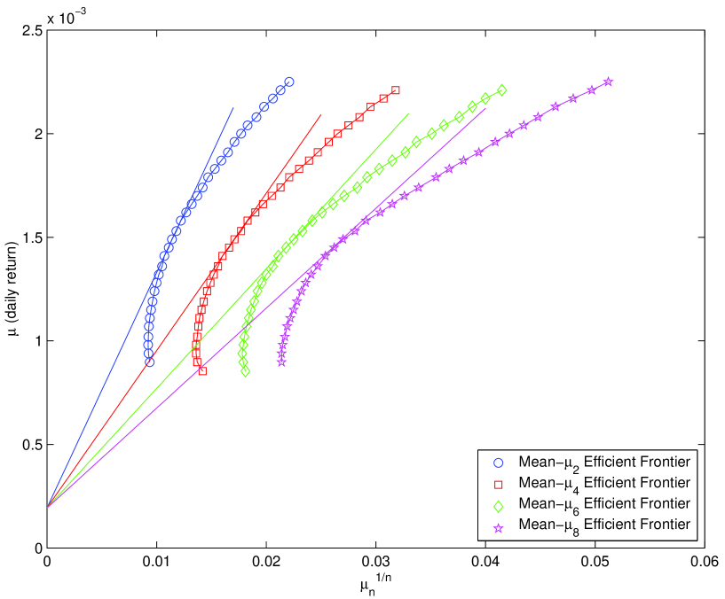
Figure 2: This figure represents the generalized efficient frontier for a portfolio made of seventeen risky assets. The optimization problem is solved numerically, using a genetic algorithm, with risk measures given respectively by the centered moments $\mu_{2},\mu_{4}$, $\mu_{6}$ and $\mu_{8}$. The straight lines are the efficient frontiers when we add to these assets a risk-free asset whose interest rate is set to 5% a year.

As an example, we have represented In figure 2, the mean-$\rho_{\alpha}$ efficient frontier for a portfolio made of seventeen assets (see appendix A for details) in the plane ($\mu,\rho_{\alpha}^{1/\alpha}$), where $\rho_{\alpha}$ represents the centered moments $\mu_{n=\alpha}$ of order $n=2,4,6$ and $8$. The efficient frontier is concave, as expected from the nature of the optimization problem (13). For a given value of the expected return $\mu$, we observe that the amount of risk measured by $\mu_{n}^{1/n}$ increases with $n$, so that there is an additional price to pay for earning more: not only the $\mu_{2}$-risk increases, as usual according to Markowitz’s theory, but the large risks increases faster, the more so, the larger $n$ is. This means that, in this example, the large risks increases more rapidly than the small risks, as the required return increases. This is an important empirical result that has obvious implications for portfolio selection and risk assessment. For instance, let us consider an efficient portfolio whose expected (daily) return equals 0.12%, which gives an annualized return equal to 30%. We can see in table 1 that the typical fluctuations around the expected return are about twice larger when measured by $\mu_{6}$ compared with $\mu_{2}$ and that they are 1.5 larger when measured with $\mu_{8}$ compared with $\mu_{4}$.

3.2 Efficient frontier with a risk-free asset

Let us now assume the existence of a risk-free asset $X_{0}$. The optimization problem with the same set of constraints as previoulsy can be written as:

$$\left\{\begin{array}[]{l}\inf_{w_{i}\in[0,1]}\rho_{\alpha}(\{w_{i}\})\\ \sum_{i\geq 0}w_{i}=1\\ \sum_{i\geq 0}w_{i}\mu(i)=\mu~{},\\ w_{i}\geq 0,~{}~{}~{}~{}\forall i>0,\end{array}\right.$$ (14)

This optimization problem can be solved exactly. Indeed, due to existence of a risk-free asset, the normalization condition $\sum w_{i}=1$ is not-constraining since one can always adjust, by lending or borrowing money, the fraction $w_{0}$ to a value satisfying the normalization condition. Thus, as shown in appendix B, the efficient frontier is a straight line in the plane $(\mu,{\rho_{\alpha}}^{1/\alpha})$, with positive slope and whose intercept is given by the value of the risk-free interest rate:

$$\mu=\mu_{0}+\xi\cdot{\rho_{\alpha}}^{1/\alpha}~{},$$ (15)

where $\xi$ is a coefficient given explicitely below. This result is very natural when $\rho_{\alpha}$ denotes the variance, since it is then nothing but [Markovitz (1959)]’s result. But in addition, it shows that the mean-variance result can be generalized to every mean-$\rho_{\alpha}$ optimal portfolios.

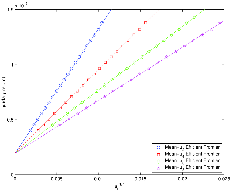
Figure 3: This figure represents the generalized efficient frontier for a portfolio made of seventeen risky assets and a risk-free asset whose interest rate is set to 5% a year. The optimization problem is solved numerically, using a genetic algorithm, with risk measures given by the centered moments $\mu_{2},\mu_{4}$, $\mu_{6}$ and $\mu_{8}$.

We present in figure 3 the results given by numerical simulations. The set of assets is the same as before and the risk-free interest rate has been set to $5\%$ a year. The optimization procedure has been performed using a genetic algorithm on the risk measure given by the centered moments $\mu_{2},\mu_{4},\mu_{6}$ and $\mu_{8}$. As expected, we observe three increasing straight lines, whose slopes monotonically decay with the order of the centered moment under consideration. Below, we will discuss this property in greater detail.

3.3 Two funds separation theorem

The two funds separation theorem is a well-known result associated with the mean-variance efficient portfolios. It results from the concavity of the Markovitz’s efficient frontier for portfolios made of risky assets only. It states that, if the investors can choose between a set of risky assets and a risk-free asset, they invest a fraction $w_{0}$ of their wealth in the risk-free asset and the fraction $1-w_{0}$ in a portfolio composed only with risky assets. This risky portofolio is the same for all the investors and the fraction $w_{0}$ of wealth invested in the risk-free asset depends on the risk aversion of the investor or on the amount of economic capital an institution must keep aside due to the legal requirements insuring its solvency at a given confidence level. We shall see that this result can be generalized to any mean-$\rho_{\alpha}$ efficient portfolio.

Indeed, it can be shown (see appendix B) that the weights of the optimal portfolios that are solutions of (14) are given by:

$$w_{0}^{*} = w_{0},$$ (16)

$$w_{i}^{*} = (1-w_{0})\cdot\tilde{w}_{i},~{}~{}~{}~{}~{}i\geq 1,$$ (17)

where the $\tilde{w}_{i}$’s are constants such that $\sum\tilde{w}_{i}=1$ and whose expressions are given appendix B. Thus, denoting by $\Pi$ the portfolio only made of risky assets whose weights are the $\tilde{w}_{i}$’s, the optimal portfolios are the linear combination of the risk-free asset, with weight $w_{0}$, and of the portfolio $\Pi$, with weigth $1-w_{0}$. This result generalizes the mean-variance two fund theorem to any mean-$\rho_{\alpha}$ efficient portfolio.

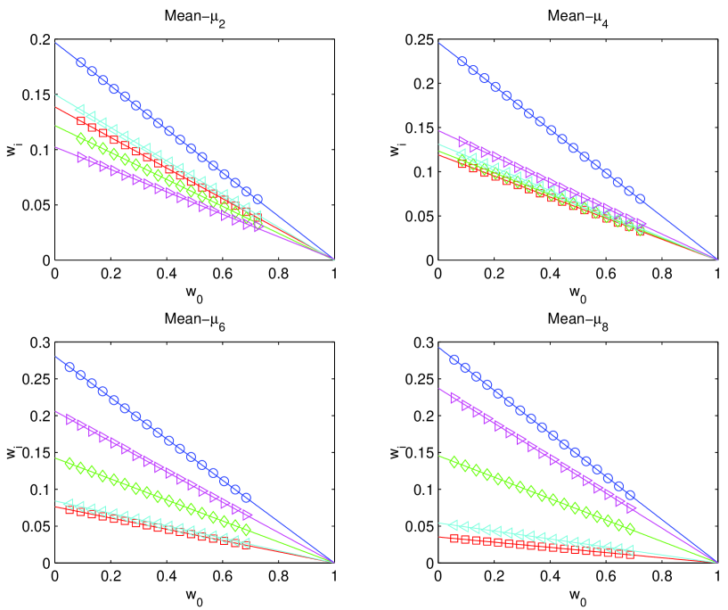
Figure 4: Dependence of the five largest weights of risky assets in the efficient portfolios found in figure 3 as a function of the weight $w_{0}$ invested in the risk-free asset, for the four risk measures given by the centered moments $\mu_{2},\mu_{4}$, $\mu_{6}$ and $\mu_{8}$. The same symbols always represent the same asset.

To check numerically this prediction, figure 4 represents the five largest weights of assets in the portfolios previously investigated as a function of the weight of the risk-free asset, for the four risk measures given by the centered moments $\mu_{2},\mu_{4},\mu_{6}$ and $\mu_{8}$. One can observe decaying straight lines that intercept the horizontal axis at $w_{0}=1$, as predicted by equations (16-17).

In figure 2, the straight lines representing the efficient portfolios with a risk-free asset are also represented. They are tangent to the efficient frontiers without risk-free asset. This is natural since the efficient portfolios with the risk-free asset are the weighted sum of the risk-free asset and the optimal portfolio $\Pi$ only made of risky assets. Since $\Pi$ also belongs to the efficient frontier without risk-free asset, the optimum is reached when the straight line describing the efficient frontier with a risk-free asset and the (concave) curve of the efficient frontier without risk-free asset are tangent.

3.4 Influence of the risk-free interest rate

Figure 3 has shown that the slope of the efficient frontier (with a risk-free asset) decreases when the order $n$ of the centered moment used to measure risks increases. This is an important qualitative properties of the risk measures offered by the centered moments, as this means that higher and higher large risks are sampled under increasing imposed return.

Is it possible that the largest risks captured by the high-order centered moments could increase at a slower rate than the small risks embodied in the small-order centered cumulants? For instance, is it possible for the slope of the mean-$\mu_{6}$ efficient frontier to be larger than the slope of the mean-$\mu_{4}$ frontier? This is an important question as it conditions the relative costs in terms of the panel of risks under increasing specified returns. To address this question, consider figure 2. Changing the value of the risk-free interest rate amounts to move the intercept of the straight lines along the ordinate axis so as to keep them tangent to the efficient frontiers without risk-free asset. Therefore, it is easy to see that, in the situation depicted in figure 2, the slope of the four straight lines will always decay with the order of the centered moment.

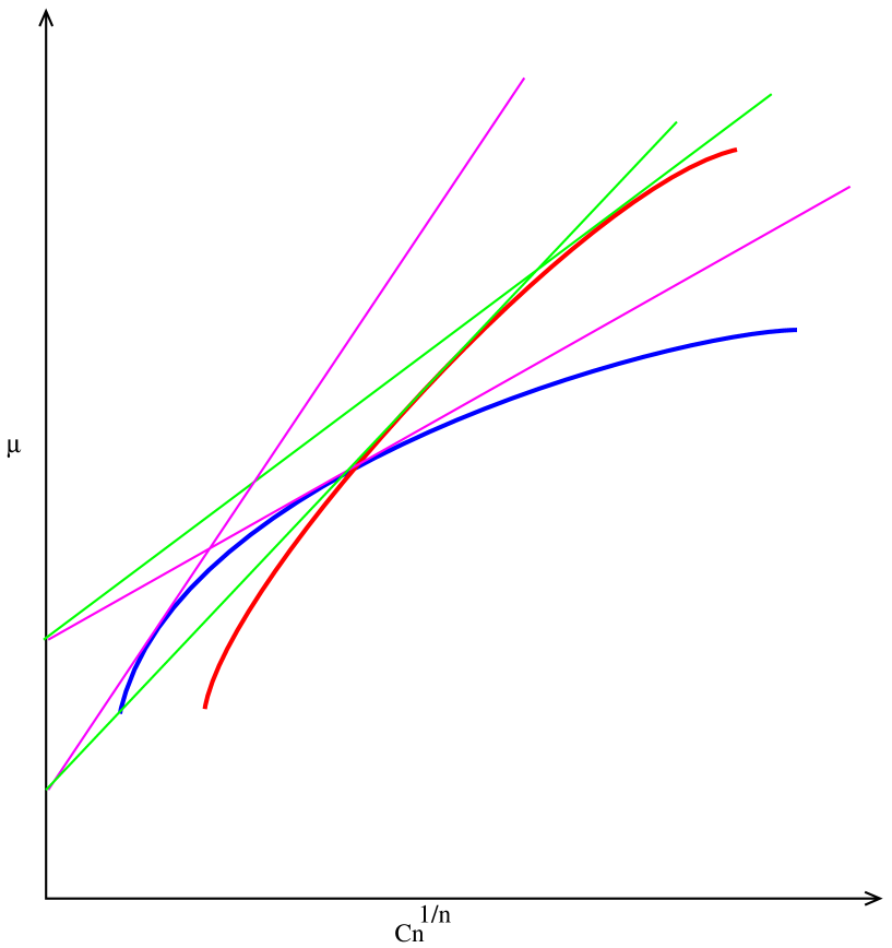
Figure 5: The dark and grey thick curves represent two efficient frontiers for a portfolio without risk-free interest rate obtained with two measures of risks. The dark and grey thin straight lines represent the efficient frontiers in the presence of a risk-free asset, whose value is given by the intercept of the straight lines with the ordinate axis. This illustrates the existence of an inversion of the dependence of the slope of the efficient frontier with risk-free asset as a function of the order $n$ of the measures of risks, which can occur only when the efficient frontiers without risk-free asset cross each other.

In order to observe an inversion in the order of the slopes, it is necessary and sufficient that the efficient frontiers without risk-free asset cross each other. This assertion is proved by visual inspection of figure 5. Can we observe such crossing of efficient frontiers? In the most general case of risk measure, nothing forbids this occurence. Nonetheless, we think that this kind of behavior is not realistic in a financial context since, as said above, it would mean that the large risks could increase at a slower rate than the small risks, implying an irrational behavior of the economic agents.

4 Classification of the assets and of portfolios

Let us consider two assets or portfolios $X_{1}$ and $X_{2}$ with different expected returns $\mu(1)$, $\mu(2)$ and different levels of risk measured by $\rho_{\alpha}(X_{1})$ and $\rho_{\alpha}(X_{2})$. An important question is then to be able to compare these two assets or portfolios. The most general way to perform such a comparison is to refer to decision theory and to calculate the utility of each of them. But, as already said, the utility function of an agent is generally not known, so that other approaches have to be developed. The simplest solution is to consider that the couple (expected return, risk measure) fully characterizes the behavior of the economic agent and thus provides a sufficiently good approximation for her utility function.

In the [Markovitz (1959)]’s world for instance, the preferences of the agents are summarized by the two first moments of the distribution of assets returns. Thus, as shown by [Sharpe (1966), Sharpe (1994)] a simple way to synthetize these two parameters, in order to get a measure of the performance of the assets or portfolios, is to build the ratio of the expected return $\mu$ (minus the risk free interest rate) over the standard deviation $\sigma$:

$$S=\frac{\mu-\mu_{0}}{\sigma},$$ (18)

which is the so-called Sharpe ratio and simply represents the amount of expected return per unit of risk, measured by the standard deviation. It is an increasing function of the expected return and a decreasing function of the level of risk, which is natural for risk-averse or prudential agent.

4.1 The risk-adjustment approach

This approach can be generalized to any type of risk measures (see [Dowd (2000)], for instance) and thus allows for the comparison of assets whose risks are not well accounted for by the variance (or the standard deviation). Indeed, instead of considering the variance, which only accounts for the small risks, one can build the ratio of the expected return over any risk measure. In fact, looking at the equation (113) in appendix B, the expression

$$\frac{\mu-\mu_{0}}{\rho_{\alpha}(X)^{1/\alpha}},$$ (19)

naturally arises and is constant for every efficient portfolios. In this expression, $\alpha$ denotes the coefficient of homogeneity of the risk measure. It is nothing but a simple generalisation of the usual Sharpe ratio. Indeed, when $\rho_{\alpha}$ is given by the variance $\sigma^{2}$, the expression above recovers the Sharpe ratio. Thus, once the portfolio manager has chosen his measure of fluctuations $\rho_{\alpha}$, he can build a consistent risk-adjusted performance measure, as shown by (19).

As just said, these generalized Sharpe ratios are constant for every efficient portfolios. In fact, they are not only constant but also maximum for every efficient portfolios, so that looking for the portfolio with maximum generalized Sharpe ratio yields the same optimal portfolios as those found with the whole optimization program solved in the previous section.

As an illutration, table 2 gives the risk-adjusted performance of the set of seventeen assets already studied, for several risk measures. We have considered the three first even order centered moments (columns 2 to 4) and the three first even order cumulants (columns 2, 5 and 6) as fluctuation measures. Obviously the second order centered moment and the second order cumulant are the same, and give again the usual Sharpe ratio (18). The assets have been sorted with respect to their Sharpe Ratio.

The first point to note is that the rank of an asset in terms of risk-adjusted perfomance strongly depends on the risk measure under consideration. The case of MCI Worldcom is very striking in this respect. Indeed, according to the usual Sharpe ratio, it appears in the 12^th position with a value larger than $0.04$ while according to the other measures it is the last asset of our selection with a value lower than $0.02$.

The second interesting point is that, for a given asset, the generalize Sharpe ratio is always a decreasing function of the order of the considered centered moment. This is not particular to our set of assets since we can prove that

$$\left({\rm E}\left[|X|^{p}\right]\right)^{1/p}\geq\left({\rm E}\left[|X|^{q}\right]\right)^{1/q},$$ (20)

so that

$$\forall p>q,~{}~{}~{}\frac{\mu-\mu_{0}}{\left({\rm E}\left[|X|^{p}\right]\right)^{1/p}}\leq\frac{\mu-\mu_{0}}{\left({\rm E}\left[|X|^{q}\right]\right)^{1/q}}.$$ (21)

On the contrary, when the cumulants are used as risk measures, the generalized Sharpe ratios are not monotonically decreasing, as exhibited by Procter & Gamble for instance. This can be surprising in view of our previous remark that the larger is the order of the moments involved in a risk measure, the larger are the fluctuations it is accounting for. Extrapolating this property to cumulants, it would mean that Procter & Gamble presents less large risks according to $C_{6}$ than according to $C_{4}$, while according to the centered moments, the reverse evolution is observed.

Thus, the question of the coherence of the cumulants as measures of fluctuations may arise. And if we accept that such measures are coherent, what are the implications on the preferences of the agents employing such measures ? To answer this question, it is informative to express the cumulants as a function of the moments. For instance, let us consider the fourth order cumulant

$$C_{4} = \mu_{4}-3\cdot{\mu_{2}}^{2},$$ (22)

$$= \mu_{4}-3\cdot{C_{2}}^{2}~{}.$$ (23)

An agent assessing the fluctuations of an asset with respect to $C_{4}$ presents aversion for the fluctuations quantified by the fourth central moment $\mu_{4}$ – since $C_{4}$ increases with $\mu_{4}$ – but is attracted by the fluctuations measured by the variance - since $C_{4}$ decreases with $\mu_{2}$. This behavior is not irrational since it remains globally risk-averse. Indeed, it depicts an agent which tries to avoid the larger risks but is ready to accept the smallest ones.

This kind of behavior is characteristic of any agent using the cumulants as risk measures. It thus allows us to understand why Procter & Gamble is more attractive for an agent sentitive to $C_{6}$ than for an agent sentitive to $C_{4}$. From the expression of $C_{6}$, we remark that the agent sensitive to this cumulant is risk-averse with respect to the fluctuations mesured by $\mu_{6}$ and $\mu_{2}$ but is risk-seeker with respect to the fluctuations mesured by $\mu_{4}$ and $\mu_{3}$. Then, is this particular case, the later ones compensate the former ones.

It also allows us to understand from a behavioral stand-point why it is possible to “have your cake and eat it too” in the sense of [Andersen and Sornette (2001)], that is, why, when the cumulants are choosen as risk measures, it may be possible to increase the expected return of a portfolio while lowering its large risks, or in other words, why its generalized Sharpe ratio may increase when one consider larger cumulants to measure its risks. We will discuus this point again in section 9.

4.2 Marginal risk of an asset within a portofolio

Another important question that arises is the contribution of a given asset to the risk of the whole portfolio. Indeed, it is crucial to know whether the risk is homogeneously shared by all the assets of the portfolio or if it is only held by a few of them. The quality of the diversification is then at stake. Moreover, this also allows for the sensitivity analysis of the risk of the portfolio with respect to small changes in its composition, which is of practical interest since it can prevent us from recalculating the whole risk of the portfolio after a small re-adjustment of its composition.

Due to the homogeneity property of the fluctuation measures and to Euler’s theorem for homogeneous functions, we can write that

$$\rho(\{w_{1},\cdots,w_{N}\})=\frac{1}{\alpha}\sum_{i_{1}}^{N}w_{i}\cdot\frac{\partial\rho}{\partial w_{i}},$$ (24)

provided the risk measure $\rho$ is differentiable which will be assumed in all the sequel. In this expression, the coefficient $\alpha$ again denotes the degree of homogeneity of the risk measure $\rho$

This relation simply shows that the amount of risk brought by one unit of the asset $i$ in the portfolio is given by the first derivative of the risk of the portfolio with respect to the weight $w_{i}$ ot this asset. Thus, $\alpha^{-1}\cdot\frac{\partial\rho}{\partial w_{i}}$ represents the marginal amount of risk of asset $i$ in the portfolio. It is then easy to check that, in a portfolio with minimum risk, irrespective of the expected return, the weight of each asset is such that the marginal risks of the assets in the portfolio are equal.

5 A new equilibrum model for asset prices

Using the portfolio selection method explained in the two previous sections, we now present an equilibrium model generalizing the original Capital Asset Pricing Model developed by [Sharpe (1964), Lintner (1965), Mossin (1966)]. Many generalizations have already been proposed to account for the fat-tailness of the assets return distributions, which led to the multi-moments CAPM. For instance [Rubinstein (1973)] and [Krauss and Lintzenberger (1976)] or [Lim (1989)] and [Harvey and Siddique (2000)] have underlined and tested the role of the asymmetry in the risk premium by accounting for the skewness of the distribution of returns. More recently, [Fang and Lai (1997)] and [Hwang and Satchell (1999)] have introduced a four-moments CAPM to take into account the letpokurtic behavior of the assets return distributions. Many other extentions have been presented such as the VaR-CAPM (see [Alexander and Baptista (2002)]) or the Distributional-CAPM by [Polimenis (2002)]. All these generalization become more and more complicated and not do not provide necessarily more accurate prediction of the expected returns.

Here, we will assume that the relevant risk measure is given by any measure of fluctuations previously presented that obey the axioms I-IV of section 2. We will also relax the usual assumption of an homogeneous market to give to the economic agents the choice of their own risk measure: some of them may choose a risk measure which put the emphasis on the small fluctuations while others may prefer those which account for the large ones. We will show that, in such an heterogeneous market, an equilibrium can still be reached and that the excess returns of individual stocks remain proportional to the market excess return.

For this, we need the following assumptions about the market:

• H1: We consider a one-period market, such that all the positions held at the begining of a period are cleared at the end of the same period.

• H2: The market is perfect, i.e., there are no transaction cost or taxes, the market is efficient and the investors can lend and borrow at the same risk-free rate $\mu_{0}$.

We will now add another assumption that specifies the behavior of the agents acting on the market, which will lead us to make the distinction between homogeneous and heterogeneous markets.

5.1 Equilibrium in a homogeneous market

The market is said to be homogeneous if all the agents acting on this market aim at fulfilling the same objective. This means that:

• H3-1: all the agents want to maximize the expected return of their portfolio at the end of the period under a given constraint of measured risk, using the same measure of risks $\rho_{\alpha}$ for all of them.

In the special case where $\rho_{\alpha}$ denotes the variance, all the agents follow a Markovitz’s optimization procedure, which leads to the CAPM equilibrium, as proved by [Sharpe (1964)]. When $\rho_{\alpha}$ represents the centered moments, we will be led to the market equilibrium described by [Rubinstein (1973)]. Thus, this approach allows for a generalization of the most popular asset pricing in equilibirum market models.

When all the agents have the same risk function $\rho_{\alpha}$, whatever $\alpha$ may be, we can assert that they have all a fraction of their capital invested in the same portfolio $\Pi$, whose composition is given in appendix B, and the remaining in the risk-free asset. The amount of capital invested in the risky fund only depends on their risk aversion or on the legal margin requirement they have to fulfil.

Let us now assume that the market is at equilibrium, i.e., supply equals demand. In such a case, since the optimal portfolios can be any linear combinations of the risk-free asset and of the risky portfolio $\Pi$, it is straightforward to show (see appendix C) that the market portfolio, made of all traded assets in proportion of their market capitalization, is nothing but the risky portfolio $\Pi$. Thus, as shown in appendix D, we can state that, whatever the risk measure $\rho_{\alpha}$ chosen by the agents to perform their optimization, the excess return of any asset over the risk-free interest rate is proportional to the excess return of the market portfolio $\Pi$ over the risk-free interest rate:

$$\mu(i)-\mu_{0}=\beta_{\alpha}^{i}\cdot(\mu_{\Pi}-\mu_{0}),$$ (25)

where

$$\beta_{\alpha}^{i}=\cdot\left.\frac{\partial\ln\left({\rho_{\alpha}}^{\frac{1}{\alpha}}\right)}{\partial w_{i}}\right|_{w_{1}^{*},\cdots,w_{N}^{*}}~{},$$ (26)

where $w_{1}^{*},\cdots,w_{N}^{*}$ are defined in appendix D. When $\rho_{\alpha}$ denotes the variance, we recover the usual $\beta^{i}$ given by the mean-variance approach:

$$\beta^{i}=\frac{{\rm Cov}(X_{i},\Pi)}{{\rm Var}(\Pi)}.$$ (27)

Thus, the relations (25) and (26) generalize the usual CAPM formula, showing that the specific choice of the risk measure is not very important, as long as it follows the axioms I-IV characterizing the fluctuations of the distribution of asset returns.

5.2 Equilibrium in a heterogeneous market

Does this result hold in the more realistic situation of an heterogeneous market? A market will be said to be heterogeneous if the agents seek to fulfill different objectives. We thus consider the following assumption:

• H3-2: There exists N agents. Each agent $n$ is characterized by her choice of a risk measure $\rho_{\alpha}(n)$ so that she invests only in the mean-$\rho_{\alpha}(n)$ efficient portfolios.

According to this hypothesis, an agent $n$ invests a fraction of her wealth in the risk-free asset and the remaining in $\Pi_{n}$, the mean-$\rho_{\alpha}(n)$ efficient portfolio, only made of risky assets. The fraction of wealth invested in the risky fund depends on the risk aversion of each agents, which may vary from an agent to another one.

The composition of the market portfolio for such a heterogenous market is derived in appendix C. We find that the market portfolio $\Pi$ is nothing but the weighted sum of the mean-$\rho_{\alpha}(n)$ optimal portfolio $\Pi_{n}$:

$$\Pi=\sum_{n=1}^{N}\gamma_{n}\Pi_{n},$$ (28)

where $\gamma_{n}$ is the fraction of the total wealth invested in the fund $\Pi_{n}$ by the n^th agent.

Appendix D demonstrates that, for every asset $i$ and for any mean-$\rho_{\alpha}(n)$ efficient portfolio $\Pi_{n}$, for all $n$, the following equation holds

$$\mu(i)-\mu_{0}=\beta_{n}^{i}\cdot(\mu_{\Pi_{n}}-\mu_{0})~{}.$$ (29)

Multiplying these equations by $\gamma_{n}/\beta_{n}^{i}$, we get

$$\frac{\gamma_{n}}{\beta_{n}^{i}}\cdot(\mu(i)-\mu_{0})=\gamma_{n}\cdot(\mu_{\Pi_{n}}-\mu_{0}),$$ (30)

for all $n$, and summing over the different agents, we obtain

$$\left(\sum_{n}\frac{\gamma_{n}}{\beta_{n}^{i}}\right)\cdot(\mu(i)-\mu_{0})=\left(\sum_{n}\gamma_{n}\cdot\mu_{\Pi_{n}}\right)-\mu_{0},$$ (31)

so that

$$\mu(i)-\mu_{0}=\beta^{i}\cdot(\mu_{\Pi}-\mu_{0}),$$ (32)

with

$$\beta^{i}=\left(\sum_{n}\frac{\gamma_{n}}{\beta_{n}^{i}}\right)^{-1}~{}.$$ (33)

This allows us to conclude that, even in a heterogeneous market, the expected excess return of each individual stock is directly proportionnal to the expected excess return of the market portfolio, showing that the homogeneity of the market is not a key property necessary for observing a linear relationship between individual excess asset returns and the market excess return.

6 Estimation of the joint probability distribution of returns of several assets

A priori, one of the main practical advantage of [Markovitz (1959)]’s method and its generalization presented above is that one does not need the multivariate probability distribution function of the assets returns, as the analysis solely relies on the coherent measures $\rho(X)$ defined in section 2, such as the centered moments or the cumulants of all orders that can in principle be estimated empirically. Unfortunately, this apparent advantage maybe an illusion. Indeed, as underlined by [Stuart and Ord (1994)] for instance, the error of the empirically estimated moment of order $n$ is proportional to the moment of order $2n$, so that the error becomes quickly of the same order as the estimated moment itself. Thus, above $n=6$ (or may be $n=8$) it is not reasonable to estimate the moments and/or cumulants directly. Thus, the knowledge of the multivariate distribution of assets returns remains necessary. In addition, there is a current of thoughts that provides evidence that marginal distributions of returns may be regularly varying with index $\mu$ in the range 3-4 [Lux (1996), Pagan (1996), Gopikrishnan et al. (1998)], suggesting the non-existence of asymptotically defined moments and cumulants of order equal to or larger than $\mu$.

In the standard Gaussian framework, the multivariate distribution takes the form of an exponential of minus a quadratic form $X^{\prime}\Omega^{-1}X$, where $X$ is the unicolumn of asset returns and $\Omega$ is their covariance matrix. The beauty and simplicity of the Gaussian case is that the essentially impossible task of determining a large multidimensional function is reduced into the very much simpler one of calculating the $N(N+1)/2$ elements of the symmetric covariance matrix. Risk is then uniquely and completely embodied by the variance of the portfolio return, which is easily determined from the covariance matrix. This is the basis of Markovitz’s portfolio theory [Markovitz (1959)] and of the CAPM (see for instance [Merton (1990)]).

However, as is well-known, the variance (volatility) of portfolio returns provides at best a limited quantification of incurred risks, as the empirical distributions of returns have “fat tails” [Lux (1996), Gopikrishnan et al. (1998)] and the dependences between assets are only imperfectly accounted for by the covariance matrix
[Litterman and Winkelmann (1998)].

In this section, we present a novel approach based on [Sornette et al. (2000b)] to attack this problem in terms of the parameterization of the multivariate distribution of returns involving two steps: (i) the projection of the empirical marginal distributions onto Gaussian laws via nonlinear mappings; (ii) the use of an entropy maximization to construct the corresponding most parsimonious representation of the multivariate distribution.

6.1 A brief exposition and justification of the method

We will use the method of determination of multivariate distributions introduced by [Karlen (1998)] and [Sornette et al. (2000b)]. This method consists in two steps: (i) transform each return $x$ into a Gaussian variable $y$ by a nonlinear monotonous increasing mapping; (ii) use the principle of entropy maximization to construct the corresponding multivariate distribution of the transformed variables $y$.

The first concern to address before going any further is whether the nonlinear transformation, which is in principle different for each asset return, conserves the structure of the dependence. In what sense is the dependence between the transformed variables $y$ the same as the dependence between the asset returns $x$? It turns out that the notion of “copulas” provides a general and rigorous answer which justifies the procedure of [Sornette et al. (2000b)].

For completeness and use later on, we briefly recall the definition of a copula (for further details about the concept of copula see [Nelsen (1998)]). A function $C$ : $[0,1]^{n}\longrightarrow[0,1]$ is a $n$-copula if it enjoys the following properties :

• $\forall u\in[0,1]$, $C(1,\cdots,1,u,1\cdots,1)=u$ ,

• $\forall u_{i}\in[0,1]$, $C(u_{1},\cdots,u_{n})=0$ if at least one of the $u_{i}$ equals zero ,

• $C$ is grounded and $n$-increasing, i.e., the $C$-volume of every boxes whose vertices lie in $[0,1]^{n}$ is positive.

Skar’s Theorem then states that, given an $n$-dimensional distribution function $F$ with continuous marginal distributions $F_{1},\cdots,F_{n}$, there exists a unique $n$-copula $C$ : $[0,1]^{n}\longrightarrow[0,1]$ such that :

$$F(x_{1},\cdots,x_{n})=C(F_{1}(x_{1}),\cdots,F_{n}(x_{n}))~{}.$$ (34)

This elegant result shows that the study of the dependence of random variables can be performed independently of the behavior of the marginal distributions. Moreover, the following result shows that copulas are intrinsic measures of dependence. Consider $n$ continuous random variables $X_{1},\cdots,X_{n}$ with copula $C$. Then, if $g_{1}(X_{1}),\cdots,g_{n}(X_{n})$ are strictly increasing on the ranges of $X_{1},\cdots,X_{n}$, the random variables $Y_{1}=g_{1}(X_{1}),\cdots,Y_{n}=g_{n}(X_{n})$ have exactly the same copula $C$ [Lindskog (2000)]. The copula is thus invariant under strictly increasing tranformation of the variables. This provides a powerful way of studying scale-invariant measures of associations. It is also a natural starting point for construction of multivariate distributions and provides the theoretical justification of the method of determination of mutivariate distributions that we will use in the sequel.

6.2 Transformation of an arbitrary random variable into a Gaussian variable

Let us consider the return $X$, taken as a random variable characterized by the probability density $p(x)$. The transformation $y(x)$ which obtains a standard normal variable $y$ from $x$ is determined by the conservation of probability:

$$p(x)dx=\frac{1}{\sqrt{2\pi}}e^{-\frac{y^{2}}{2}}dy\;.$$ (35)

Integrating this equation from $-\infty$ and $x$, we obtain:

$$F(x)=\frac{1}{2}\left[1+\mbox{erf}\left(\frac{y}{\sqrt{2}}\right)\right]\;,$$ (36)

where $F(x)$ is the cumulative distribution of $X$:

$$F(x)=\int_{-\infty}^{x}dx^{\prime}p(x^{\prime})\;.$$ (37)

This leads to the following transformation $y(x)$:

$$y=\sqrt{2}\;\mbox{erf}^{-1}(2F(x)-1)~{},$$ (38)

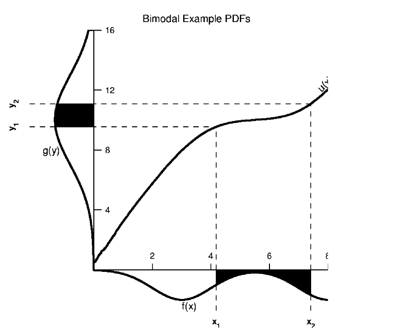
Figure 6: Schematic representation of the nonlinear mapping $Y=u(X)$ that allows one to transform a variable $X$ with an arbitrary distribution into a variable $Y$ with a Gaussian distribution. The probability densities for $X$ and $Y$ are plotted outside their respective axes. Consistent with the conservation of probability, the shaded regions have equal area. This conservation of probability determines the nonlinear mapping.

which is obvously an increasing function of $X$ as required for the application of the invariance property of the copula stated in the previous section. An illustration of the nonlinear transformation (38) is shown in figure 6. Note that it does not require any special hypothesis on the probability density $X$, apart from being non-degenerate.

In the case where the pdf of $X$ has only one maximum, we may use a simpler expression equivalent to (38). Such a pdf can be written under the so-called Von Mises parametrization [Embrechts et al. (1997)] :

$$p(x)=C\frac{f^{\prime}(x)}{\sqrt{|f(x)|}}e^{-\frac{1}{2}f(x)}\;,$$ (39)

where $C$ is a constant of normalization. For $f(x)/x^{2}\rightarrow 0$ when $|x|\rightarrow+\infty$, the pdf has a “fat tail,” i.e., it decays slower than a Gaussian at large $|x|$.

Let us now define the change of variable

$$y=sgn(x)\sqrt{|f(x)|}\;.$$ (40)

Using the relationship $p(y)=p(x)\frac{dx}{dy}$, we get:

$$p(y)=\frac{1}{\sqrt{2\pi}}e^{-\frac{y^{2}}{2}}\;.$$ (41)

It is important to stress the presence of the sign function $sgn(x)$ in equation (40), which is essential in order to correctly quantify dependences between random variables. This transformation (40) is equivalent to (38) but of a simpler implementation and will be used in the sequel.

6.3 Determination of the joint distribution : maximum entropy and Gaussian copula

Let us now consider $N$ random variables $X_{i}$ with marginal distributions $p_{i}(x_{i})$. Using the transformation (38), we define $N$ standard normal variables $Y_{i}$. If these variables were independent, their joint distribution would simply be the product of the marginal distributions. In many situations, the variables are not independent and it is necessary to study their dependence.

The simplest approach is to construct their covariance matrix. Applied to the variables $Y_{i}$, we are certain that the covariance matrix exists and is well-defined since their marginal distributions are Gaussian. In contrast, this is not ensured for the variables $X_{i}$. Indeed, in many situations in nature, in economy, finance and in social sciences, pdf’s are found to have power law tails $\sim\frac{A}{x^{1+\mu}}$ for large $|x|$. If $\mu\leq 2$, the variance and the covariances can not be defined. If $2<\mu\leq 4$, the variance and the covariances exit in principle but their sample estimators converge poorly.

We thus define the covariance matrix:

$$V=E[{\bf y}{\bf y^{t}}]\;,$$ (42)

where ${\bf y}$ is the vector of variables $Y_{i}$ and the operator $E[\cdot]$ represents the mathematical expectation. A classical result of information theory [Rao (1973)] tells us that, given the covariance matrix $V$, the best joint distribution (in the sense of entropy maximization) of the $N$ variables $Y_{i}$ is the multivariate Gaussian:

$$P({\bf y})=\frac{1}{(2\pi)^{N/2}\sqrt{\det(V)}}\exp\left(-\frac{1}{2}{\bf y^{t}}V^{-1}{\bf y}\right)\;.$$ (43)

Indeed, this distribution implies the minimum additional information or assumption, given the covariance matrix.

Using the joint distribution of the variables $Y_{i}$, we obtain the joint distribution of the variables $X_{i}$:

$$P({\bf x})=P({\bf y})\left|\frac{\partial y_{i}}{\partial x_{j}}\right|\;,$$ (44)

where $\left|\frac{\partial y_{i}}{\partial x_{j}}\right|$ is the Jacobian of the transformation. Since

$$\frac{\partial y_{i}}{\partial x_{j}}=\sqrt{2\pi}p_{j}(x_{j})e^{\frac{1}{2}y_{i}^{2}}\delta_{ij}\;,$$ (45)

we get

$$\left|\frac{\partial y_{i}}{\partial x_{j}}\right|=(2\pi)^{N/2}\prod_{i=1}^{N}p_{i}(x_{i})e^{\frac{1}{2}y_{i}^{2}}\;.$$ (46)

This finally yields

$$P({\bf x})=\frac{1}{\sqrt{\det(V)}}\exp\left(-\frac{1}{2}{\bf y_{(x)}^{t}}(V^{-1}-I){\bf y_{(x)}}\ \right)\prod_{i=1}^{N}p_{i}(x_{i})\;.$$ (47)

As expected, if the variables are independent, $V=I$, and $P({\bf x})$ becomes the product of the marginal distributions of the variables $X_{i}$.

Let $F({\bf x})$ denote the cumulative distribution function of the vector x and $F_{i}(x_{i}),i=1,...,N$ the $N$ corresponding marginal distributions. The copula $C$ is then such that

$$F(x_{1},\cdots,x_{n})=C(F_{1}(x_{1}),\cdots,F_{n}(x_{n}))~{}.$$ (48)

Differentiating with respect to $x_{1},\cdots,x_{N}$ leads to

$$P(x_{1},\cdots,x_{n})=\frac{\partial F(x_{1},\cdots,x_{n})}{\partial x_{1}\cdots\partial x_{n}}=c(F_{1}(x_{1}),\cdots,F_{n}(x_{n}))\prod_{i=1}^{N}p_{i}(x_{i})~{},$$ (49)

where

$$c(u_{1},\cdots,u_{N})=\frac{\partial C(u_{1},\cdots,u_{N})}{\partial u_{1}\cdots\partial u_{N}}$$ (50)

is the density of the copula $C$.

Comparing (50) with (47), the density of the copula is given in the present case by

$$c(u_{1},\cdots,u_{N})=\frac{1}{\sqrt{\det(V)}}\exp\left(-\frac{1}{2}{\bf y_{(u)}^{t}}(V^{-1}-I){\bf y_{(u)}}\ \right)~{},$$ (51)

which is the “Gaussian copula” with covariance matrix ${\bf V}$. This result clarifies and justifies the method of [Sornette et al. (2000b)] by showing that it essentially amounts to assume arbitrary marginal distributions with Gaussian copulas. Note that the Gaussian copula results directly from the transformation to Gaussian marginals together with the choice of maximizing the Shannon entropy under the constraint of a fixed covariance matrix. Under differents constraint, we would have found another maximum entropy copula. This is not unexpected in analogy with the standard result that the Gaussian law is maximizing the Shannon entropy at fixed given variance. If we were to extend this formulation by considering more general expressions of the entropy, such that Tsallis entropy [Tsallis (1998)], we would have found other copulas.

6.4 Empirical test of the Gaussian copula assumption

We now present some tests of the hypothesis of Gaussian copulas between returns of financial assets. This presentation is only for illustration purposes, since testing the gaussian copula hypothesis is a delicate task which has been addressed elsewhere (see [Malevergne and Sornette (2001)]). Here, as an example, we propose two simple standard methods.

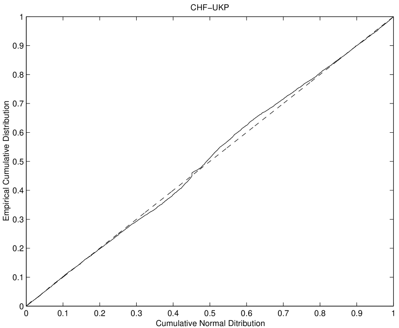
Figure 7: Quantile of the normalized sum of the Gaussianized returns of the Swiss Franc and The British Pound versus the quantile of the Normal distribution, for the time interval from Jan. 1971 to Oct. 1998. Different weights in the sum give similar results.

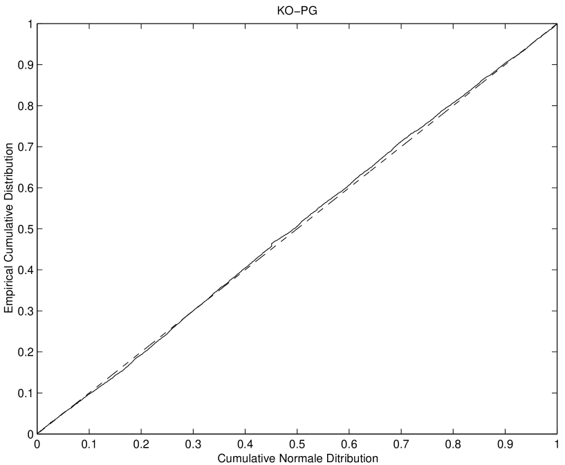
Figure 8: Quantile of the normalized sum of the Gaussianized returns of Coca-Cola and Procter&Gamble versus the quantile of the Normal distribution, for the time interval from Jan. 1970 to Dec. 2000. Different weights in the sum give similar results.

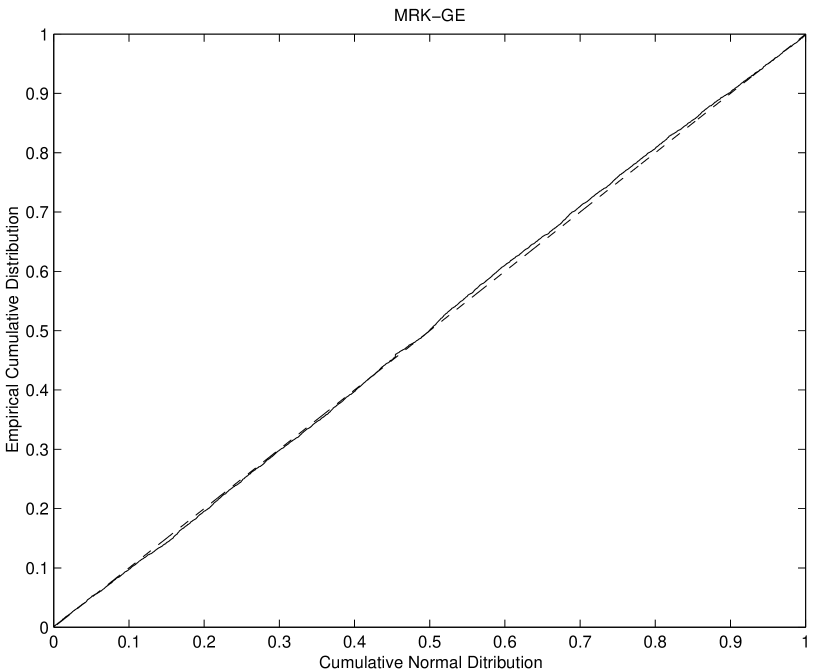
Figure 9: Quantile of the normalized sum of the Gaussianized returns of Merk and General Electric versus the quantile of the Normal distribution, for the time interval from Jan. 1970 to Dec. 2000. Different weights in the sum give similar results.

The first one consists in using the property that Gaussian variables are stable in distribution under addition. Thus, a (quantile-quantile or $Q-Q$) plot of the cumulative distribution of the sum $y_{1}+\cdots+y_{p}$ versus the cumulative Normal distribution with the same estimated variance should give a straight line in order to qualify a multivariate Gaussian distribution (for the transformed $y$ variables). Such tests on empirical data are presented in figures 7-9.

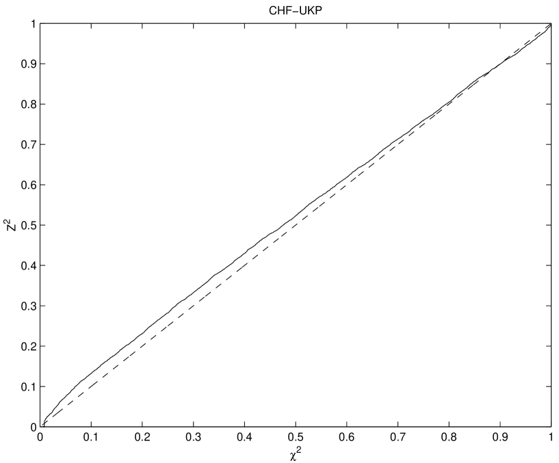
Figure 10: Cumulative distribution of $z^{2}={\bf y^{t}V^{-1}y}$ versus the cumulative distribution of chi-square (denoted $\chi^{2}$) with two degrees of freedom for the couple Swiss Franc / British Pound, for the time interval from Jan. 1971 to Oct. 1998. This $\chi^{2}$ should not be confused with the characteristic scale used in the definition of the modified Weibull distributions.

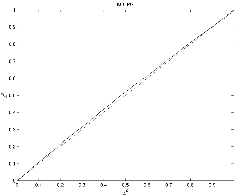
Figure 11: Cumulative distribution of $z^{2}={\bf y^{t}V^{-1}y}$ versus the cumulative distribution of the chi-square $\chi^{2}$ with two degrees of freedom for the couple Coca-Cola / Procter&Gamble, for the time interval from Jan. 1970 to Dec. 2000. This $\chi^{2}$ should not be confused with the characteristic scale used in the definition of the modified Weibull distributions.

The second test amounts to estimating the covariance matrix ${\bf V}$ of the sample we consider. This step is simple since, for fast decaying pdf’s, robust estimators of the covariance matrix are available. We can then estimate the distribution of the variable $z^{2}={\bf y^{t}V^{-1}y}$. It is well known that $z^{2}$ follows a $\chi^{2}$ distribution if ${\bf y}$ is a Gaussian random vector. Again, the empirical cumulative distribution of $z^{2}$ versus the $\chi^{2}$ cumulative distribution should give a straight line in order to qualify a multivariate Gaussian distribution (for the transformed $y$ variables). Such tests on empirical data are presented in figures 10-12.

First, one can observe that the Gaussian copula hypothesis appears better for stocks than for currencies. As discussed in [Malevergne and Sornette (2001)], this result is quite general. A plausible explanation lies in the stronger dependence between the currencies compared with that between stocks, which is due to the monetary policies limiting the fluctuations between the currencies of a group of countries, such as was the case in the European Monetary System before the unique Euro currency. Note also that the test of aggregation seems systematically more in favor of the Gaussian copula hypothesis than is the $\chi^{2}$ test, maybe due to its smaller sensitivity. Nonetheless, the very good performance of the Gaussian hypothesis under the aggregation test bears good news for a porfolio theory based on it, since by definition a portfolio corresponds to asset aggregation. Even if sums of the transformed returns are not equivalent to sums of returns (as we shall see in the sequel), such sums qualify the collective behavior whose properties are controlled by the copula.

Notwithstanding some deviations from linearity in figures 7-12, it appears that, for our purpose of developing a generalized portfolio theory, the Gaussian copula hypothesis is a good approximation. A more systematic test of this goodness of fit requires the quantification of a confidence level, for instance using the Kolmogorov test, that would allow us to accept or reject the Gaussian copula hypothesis. Such a test has been performed in [Malevergne and Sornette (2001)], where it is shown that this test is sensitive enough only in the bulk of the distribution, and that an Anderson-Darling test is preferable for the tails of the distributions. Nonetheless, the quantitative conclusions of these tests are identical to the qualitative results presented here. Some other tests would be useful, such as the multivariate Gaussianity test presented by [Richardson and Smith (1993)].

7 Choice of an exponential family to parameterize the marginal distributions

7.1 The modified Weibull distributions

We now apply these constructions to a class of distributions with fat tails, that have been found to provide a convenient and flexible parameterization of many phenomena found in nature and in the social sciences [Laherrère and Sornette (1998)]. These so-called stretched exponential distributions can be seen to be general forms of the extreme tails of product of random variables [Frisch and Sornette (1997)].

Following [Sornette et al. (2000b)], we postulate the following marginal probability distributions of returns:

$$p(x)=\frac{1}{2\sqrt{\pi}}\frac{c}{\chi^{\frac{c}{2}}}|x|^{\frac{c}{2}-1}e^{-\left(\frac{|x|}{\chi}\right)^{c}}\;,$$ (52)

where $c$ and $\chi$ are the two key parameters. A more general parameterization taking into account a possible asymmetry between negative and positive returns (thus leading to possible non-zero average return) is

$$p(x) = \frac{Q}{\sqrt{\pi}}\frac{c_{+}}{\chi_{+}^{\frac{c_{+}}{2}}}|x|^{\frac{c_{+}}{2}-1}e^{-\left(\frac{|x|}{\chi_{+}}\right)^{c_{+}}}~{}~{}~{}~{}\mbox{if}~{}x\geq 0$$ (53)

$$p(x) = \frac{1-Q}{\sqrt{\pi}}\frac{c_{-}}{\chi_{-}^{\frac{c_{-}}{2}}}|x|^{\frac{c_{-}}{2}-1}e^{-\left(\frac{|x|}{\chi_{-}}\right)^{c_{-}}}~{}~{}~{}~{}\mbox{if}~{}x<0~{},$$ (54)

where $Q$ (respectively $1-Q$) is the fraction of positive (respectively negative) returns. In the sequel, we will only consider the case $Q=\frac{1}{2}$, which is the only analytically tractable case. Thus the pdf’s asymmetry will be only accounted for by the exponents $c_{+}$, $c_{-}$ and the scale factors $\chi_{+}$, $\chi_{-}$.

We can note that these expressions are close to the Weibull distribution, with the addition of a power law prefactor to the exponential such that the Gaussian law is retrieved for $c=2$. Following [Sornette et al. (2000b), Sornette et al. (2000a), Andersen and Sornette (2001)], we call (52) the modified Weibull distribution. For $c<1$, the pdf is a stretched exponential, also called sub-exponential. The exponent $c$ determines the shape of the distribution, which is fatter than an exponential if $c<1$. The parameter $\chi$ controls the scale or characteristic width of the distribution. It plays a role analogous to the standard deviation of the Gaussian law. See chapter 6 of [Sornette(2000)] for a recent review on maximum likelihood and other estimators of such generalized Weibull distributions.

7.2 Transformation of the modified Weibull pdf into a Gaussian Law

One advantage of the class of distributions (52) is that the transformation into a Gaussian is particularly simple. Indeed, the expression (52) is of the form (39) with

$$f(x)=2\left(\frac{|x|}{\chi}\right)^{c}~{}.$$ (55)

Applying the change of variable (40) which reads

$$y_{i}=sgn(x_{i})~{}\sqrt{2}~{}\left(\frac{|x_{i}|}{\chi_{i}}\right)^{\frac{c_{i}}{2}}\;,$$ (56)

leads automatically to a Gaussian distribution.

These variables $Y_{i}$ then allow us to obtain the covariance matrix $V$ :

$$V_{ij}=\frac{2}{T}\sum_{n=1}^{T}sgn(x_{i}x_{j})\left(\frac{|x_{i}|}{\chi_{i}}\right)^{\frac{c_{i}}{2}}\left(\frac{|x_{j}|}{\chi_{j}}\right)^{\frac{c_{j}}{2}}\;,$$ (57)

and thus the multivariate distributions $P({\bf y})$ and $P({\bf x})$ :

$$P(x_{1},\cdots,x_{N})=\frac{1}{2^{N}\pi^{N/2}\sqrt{V}}~{}\exp\left[-\sum_{i,j}V_{ij}^{-1}\left(\frac{|x_{i}|}{\chi_{i}}\right)^{c/2}\left(\frac{|x_{j}|}{\chi_{j}}\right)^{c/2}\right]~{}\left(\prod_{i=1}^{N}\frac{c_{i}|x_{i}|^{c/2-1}}{\chi_{i}^{c/2}}~{}e^{-\left(\frac{|x_{i}|}{\chi}\right)^{c}}\right).$$ (58)

Similar transforms hold, mutatis mutandis, for the asymmetric case. Indeed, for asymmetric assets of interest for financial risk managers, the equations (53) and (54) yields the following change of variable:

$$y_{i} = \sqrt{2}~{}\left(\frac{x_{i}}{\chi_{i}^{+}}\right)^{\frac{c_{i}^{+}}{2}}~{}~{}{\rm and}~{}~{}x_{i}\geq 0,$$ (59)

$$y_{i} = -\sqrt{2}~{}\left(\frac{|x_{i}|}{\chi_{i}^{-}}\right)^{\frac{c_{i}^{-}}{2}}~{}~{}{\rm and}~{}~{}x_{i}<0~{}.$$ (60)

This allows us to define the correlation matrix $V$ and to obtain the multivariate distribution $P({\bf x})$, generalizing equation (58) for asymmetric assets. Since this expression is rather cumbersome and nothing but a straightforward generalization of (58), we do not write it here.

7.3 Empirical tests and estimated parameters

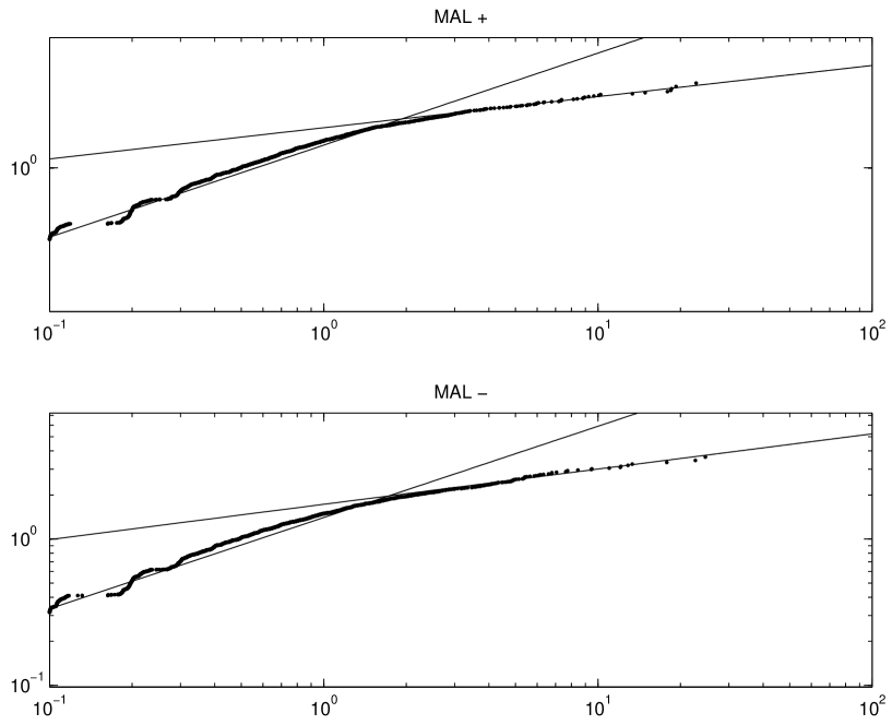
Figure 13: Graph of Gaussianized Malaysian Ringgit returns versus Malaysian Ringgit returns, for the time interval from Jan. 1971 to Oct. 1998. The upper graph gives the positive tail and the lower one the negative tail. The two straight lines represent the curves $y=\sqrt{2}\left(\frac{x}{\langle\chi_{\pm}\rangle}\right)^{\langle c_{\pm}\rangle}$ and $y=\sqrt{2}\left(\frac{x}{\chi_{\pm}}\right)^{c_{\pm}}$

In order to test the validity of our assumption, we have studied a large basket of financial assets including currencies and stocks. As an example, we present in figures 13 to 17 typical log-log plot of the transformed return variable $Y$ versus the return variable $X$ for a certain number of assets. If our assumption was right, we should observe a single straight line whose slope is given by $c/2$. In contrast, we observe in general two approximately linear regimes separated by a cross-over. This means that the marginal distribution of returns can be approximated by two modified Weibull distributions, one for small returns which is close to a Gaussian law and one for large returns with a fat tail. Each regime is depicted by its corresponding straight line in the graphs. The exponents $c$ and the scale factors $\chi$ for the different assets we have studied are given in tables 3 for currencies and 4 for stocks. The coefficients within brackets are the coefficients estimated for small returns while the non-bracketed coefficients correspond to the second fat tail regime.

The first point to note is the difference between currencies and stocks. For small as well as for large returns, the exponents $c_{-}$ and $c_{+}$ for currencies (excepted Poland and Thailand) are all close to each other. Additional tests are required to establish whether their relatively small differences are statistically significant. Similarly, the scale factors are also comparable. In contrast, many stocks exhibit a large asymmetric behavior for large returns with $c_{+}-c_{-}\gtrsim 0.5$ in about one-half of the investigated stocks. This means that the tails of the large negative returns (“crashes”)  are often much fatter than those of the large positive returns (“rallies”).

The second important point is that, for small returns, many stocks have an exponent $\langle c_{+}\rangle\approx\langle c_{-}\rangle\simeq 2$ and thus have a behavior not far from a pure Gaussian in the bulk of the distribution, while the average exponent for currencies is about $1.5$ in the same “small return” regime. Therefore, even for small returns, currencies exhibit a strong departure from Gaussian behavior.

In conclusion, this empirical study shows that the modified Weibull parameterization, although not exact on the entire range of variation of the returns $X$, remains consistent within each of the two regimes of small versus large returns, with a sharp transition between them. It seems especially relevant in the tails of the return distributions, on which we shall focus our attention next.

8 Cumulant expansion of the portfolio return distribution

8.1 link between moments and cumulants

Before deriving the main result of this section, we recall a standard relation between moments and cumulants that we need below.

The moments $M_{n}$ of the distribution $P$ are defined by

$$\hat{P}(k)=\sum_{n=0}^{+\infty}\frac{(ik)^{n}}{n!}M_{n}~{},$$ (61)

where $\hat{P}$ is the characteristic function, i.e., the Fourier transform of $P$ :

$$\hat{P}(k)=\int_{-\infty}^{+\infty}dS~{}P(S)e^{ikS}~{}.$$ (62)

Similarly, the cumulants $C_{n}$ are given by

$$\hat{P}(k)=\exp\left(\sum_{n=1}^{+\infty}\frac{(ik)^{n}}{n!}C_{n}\right)~{}.$$ (63)

Differentiating $n$ times the equation

$$\ln\left(\sum_{n=0}^{+\infty}\frac{(ik)^{n}}{n!}M_{n}\right)=\sum_{n=1}^{+\infty}\frac{(ik)^{n}}{n!}C_{n}\;,$$ (64)

we obtain the following recurrence relations between the moments and the cumulants :

$$M_{n} = \sum_{p=0}^{n-1}{{n-1}\choose{p}}M_{p}C_{n-p}\;,$$ (65)

$$C_{n} = M_{n}-\sum_{p=1}^{n-1}{{n-1}\choose{n-p}}C_{p}M_{n-p}\;.$$ (66)

In the sequel, we will first evaluate the moments, which turns out to be easier, and then using eq (66) we will be able to calculate the cumulants.

8.2 Symmetric assets

We start with the expression of the distribution of the weighted sum of $N$ assets :

$$P_{S}(s)=\int_{R^{N}}d{\bf x}\;P({\bf x})\delta(\sum_{i=1}^{N}w_{i}x_{i}-s)\;,$$ (67)

where $\delta(\cdot)$ is the Dirac distribution. Using the change of variable (40), allowing us to go from the asset returns $X_{i}$’s to the transformed returns $Y_{i}$’s, we get

$$P_{S}(s)=\frac{1}{(2\pi)^{N/2}\sqrt{\det(V)}}\int_{R^{N}}d{\bf y}\;e^{-\frac{1}{2}{\bf y^{t}}V^{-1}{\bf y}}\;\delta(\sum_{i=1}^{N}w_{i}sgn(y_{i})f^{-1}(y_{i}^{2})-s)\;.$$ (68)

Taking its Fourier transform $\hat{P}_{S}(k)=\int dsP_{S}(s)e^{iks}$, we obtain

$$\hat{P}_{S}(k)=\frac{1}{(2\pi)^{N/2}\sqrt{\det(V)}}\int_{R^{N}}d{\bf y}\;e^{-\frac{1}{2}{\bf y^{t}}V^{-1}{\bf y}+ik\sum_{i=1}^{N}w_{i}sgn(y_{i})f^{-1}(y_{i}^{2})}\;,$$ (69)

where $\hat{P}_{S}$ is the characteristic function of $P_{S}$.

In the particular case of interest here where the marginal distributions of the variables $X_{i}$’s are the modified Weibull pdf,

$$f^{-1}(y_{i})=\chi_{i}|\frac{y_{i}}{\sqrt{2}}|^{q_{i}}$$ (70)

with

$$q_{i}=2/c_{i}~{},$$ (71)

the equation (69) becomes

$$\hat{P}_{S}(k)=\frac{1}{(2\pi)^{N/2}\sqrt{\det(V)}}\int_{R^{N}}d{\bf y}\;e^{-\frac{1}{2}{\bf y^{t}}V^{-1}{\bf y}+ik\sum_{i=1}^{N}w_{i}sgn(y_{i})\chi_{i}|\frac{y_{i}}{\sqrt{2}}|^{q_{i}}}\;.$$ (72)

The task in front of us is to evaluate this expression through the determination of the moments and/or cumulants.

8.2.1 Case of independent assets

In this case, the cumulants can be obtained explicitely [Sornette et al. (2000b)]. Indeed, the expression (72) can be expressed as a product of integrals of the form

$$\int_{0}^{+\infty}du\;e^{-\frac{u^{2}}{2}+ikw_{i}\chi_{i}\left(\frac{u}{\sqrt{2}}\right)^{q_{i}}}\;.$$ (73)

We obtain

$$C_{2n}=\sum_{i=1}^{N}c(n,q_{i})(\chi_{i}w_{i})^{2n}\;,$$ (74)

and

$$c(n,q_{i})=(2n)!\left\{\sum_{p=0}^{n-2}(-1)^{n}\frac{\Gamma\left(q_{i}(n-p)+\frac{1}{2}\right)}{(2n-2p)!\pi^{1/2}}\left[\frac{\Gamma\left(q_{i}+\frac{1}{2}\right)}{2!\pi^{1/2}}\right]^{p}-\frac{(-1)^{n}}{n}\left[\frac{\Gamma\left(q_{i}+\frac{1}{2}\right)}{2!\pi^{1/2}}\right]^{n}\right\}\;.$$ (75)

Note that the coefficient $c(n,q_{i})$ is the cumulant of order $n$ of the marginal distribution (52) with $c=2/q_{i}$ and $\chi=1$. The equation (74) expresses simply the fact that the cumulants of the sum of independent variables is the sum of the cumulants of each variable. The odd-order cumulants are zero due to the symmetry of the distributions.

8.2.2 Case of dependent assets

Here, we restrict our exposition to the case of two random variables. The case with $N$ arbitrary can be treated in a similar way but involves rather complex formulas. The equation (72) reads

$$\hat{P}_{S}(k)=\frac{1}{2\pi\sqrt{1-\rho^{2}}}\int dy_{1}dy_{2}~{}\exp\left[-\frac{1}{2}y^{t}V^{-1}y+ik\left(\chi_{1}w_{1}sgn(y_{1})\left|\frac{y_{1}}{\sqrt{2}}\right|^{q_{1}}+\right.\right.{}$$

$$\left.\left.+\chi_{2}w_{2}sgn(y_{2})\left|\frac{y_{2}}{\sqrt{2}}\right|^{q_{2}}\right)\right]~{},$$ (76)

and we can show (see appendix E) that the moments read

$$M_{n}=\sum_{p=0}^{n}{n\choose p}w_{1}^{p}w_{2}^{n-p}\gamma_{q_{1}q_{2}}(n,p)~{},$$ (77)

with

$$\gamma_{q_{1}q_{2}}(2n,2p) = \chi_{1}^{2p}\chi_{2}^{2(n-p)}\frac{\Gamma\left(q_{1}p+\frac{1}{2}\right)\Gamma\left(q_{2}(n-p)+\frac{1}{2}\right)}{\pi}~{}{{}_{2}F_{1}}\left(-q_{1}p,-q_{2}(n-p);\frac{1}{2};\rho^{2}\right)\;,$$ (78)

$$\gamma_{q_{1}q_{2}}(2n,2p+1) = 2\chi_{1}^{2p+1}\chi_{2}^{2(n-p)-1}\frac{\Gamma\left(q_{1}p+1+\frac{q_{1}}{2}\right)\Gamma\left(q_{2}(n-p)+1-\frac{q_{2}}{2}\right)}{\pi}\rho~{}{{}_{2}F_{1}}\left(-q_{1}p-\frac{q_{1}-1}{2},\right.$$ (79)

$$\left.,-q_{2}(n-p)+\frac{q_{2}+1}{2};\frac{3}{2};\rho^{2}\right)~{},$$

where ${{}_{2}F_{1}}$ is an hypergeometric function.

These two relations allow us to calculate the moments and cumulants for any possible values of $q_{1}=2/c_{1}$ and $q_{2}=2/c_{2}$. If one of the $q_{i}$’s is an integer, a simplification occurs and the coefficients $\gamma(n,p)$ reduce to polynomials. In the simpler case where all the $q_{i}$’s are odd integer the expression of moments becomes :

$$M_{n}=\sum_{p=0}^{n}{n\choose p}\left(w_{1}{\chi_{1}}\right)^{p}\left(w_{2}{\chi_{2}}\right)^{n-p}\sum_{s=0}^{min\{q_{1}p,q_{2}(n-p)\}}{\rho}^{s}~{}s!~{}a_{s}^{(q_{1}p)}a_{s}^{(q_{2}(n-p))}~{},$$ (80)

with

$$a_{2p}^{(2n)} = (2p)!{2(n-p)\choose 2n}~{}(2(n-p)-1)!!=\frac{(2n)!}{2^{n-p}~{}(n-p)!}\;,$$ (81)

$$a_{2p+1}^{(2n)} = 0\;,$$ (82)

$$a_{2p}^{(2n+1)} = 0\;,$$ (83)

$$a_{2p+1}^{(2n+1)} = (2p+1)!{2(n-p)\choose 2n+1}~{}(2(n-p)-1)!!=\frac{(2n+1)!}{2^{n-p}~{}(n-p)!}\;.$$ (84)

8.3 Non-symmetric assets

In the case of asymmetric assets, we have to consider the formula (53-54), and using the same notation as in the previous section, the moments are again given by (77) with the coefficient $\gamma(n,p)$ now equal to :

$$\gamma(n,p)=\frac{(-1)^{n}(\chi_{1}^{-})^{p}(\chi_{2}^{-})^{n-p}}{4\pi}\left[\Gamma\left(\frac{q_{1}^{-}p+1}{2}\right)\Gamma\left(\frac{q_{2}^{-}(n-p)+1}{2}\right)~{}_{2}F_{1}\left(-\frac{q_{1}^{-}p}{2},-\frac{q_{2}^{-}(n-p)}{2};\frac{1}{2};\rho^{2}\right)+\right.$$

$$\left.+2\Gamma\left(\frac{q_{1}^{-}p}{2}+1\right)\Gamma\left(\frac{q_{2}^{-}(n-p)}{2}+1\right)\rho~{}_{2}F_{1}\left(-\frac{q_{1}^{-}p-1}{2},-\frac{q_{2}^{-}(n-p)-1}{2};\frac{3}{2};\rho^{2}\right)\right]+$$

$$+\frac{(-1)^{p}(\chi_{1}^{-})^{p}(\chi_{2}^{+})^{n-p}}{4\pi}\left[\Gamma\left(\frac{q_{1}^{-}p+1}{2}\right)\Gamma\left(\frac{q_{2}^{+}(n-p)+1}{2}\right)~{}_{2}F_{1}\left(-\frac{q_{1}^{-}p}{2},-\frac{q_{2}^{+}(n-p)}{2};\frac{1}{2};\rho^{2}\right)+\right.$$

$$\left.-2\Gamma\left(\frac{q_{1}^{-}p}{2}+1\right)\Gamma\left(\frac{q_{2}^{+}(n-p)}{2}+1\right)\rho~{}_{2}F_{1}\left(-\frac{q_{1}^{-}p-1}{2},-\frac{q_{2}^{+}(n-p)-1}{2};\frac{3}{2};\rho^{2}\right)\right]+$$

$$+\frac{(-1)^{n-p}(\chi_{1}^{+})^{p}(\chi_{2}^{-})^{n-p}}{4\pi}\left[\Gamma\left(\frac{q_{1}^{+}p+1}{2}\right)\Gamma\left(\frac{q_{2}^{-}(n-p)+1}{2}\right)~{}_{2}F_{1}\left(-\frac{q_{1}^{+}p}{2},-\frac{q_{2}^{-}(n-p)}{2};\frac{1}{2};\rho^{2}\right)+\right.$$

$$\left.-2\Gamma\left(\frac{q_{1}^{+}p}{2}+1\right)\Gamma\left(\frac{q_{2}^{-}(n-p)}{2}+1\right)\rho~{}_{2}F_{1}\left(-\frac{q_{1}^{+}p-1}{2},-\frac{q_{2}^{-}(n-p)-1}{2};\frac{3}{2};\rho^{2}\right)\right]+$$

$$+\frac{(\chi_{1}^{+})^{p}(\chi_{2}^{+})^{n-p}}{4\pi}\left[\Gamma\left(\frac{q_{1}^{+}p+1}{2}\right)\Gamma\left(\frac{q_{2}^{+}(n-p)+1}{2}\right)~{}_{2}F_{1}\left(-\frac{q_{1}^{+}p}{2},-\frac{q_{2}^{+}(n-p)}{2};\frac{1}{2};\rho^{2}\right)+\right.$$

$$\left.+2\Gamma\left(\frac{q_{1}^{+}p}{2}+1\right)\Gamma\left(\frac{q_{2}^{+}(n-p)}{2}+1\right)\rho~{}_{2}F_{1}\left(-\frac{q_{1}^{+}p-1}{2},-\frac{q_{2}^{+}(n-p)-1}{2};\frac{3}{2};\rho^{2}\right)\right]~{}.$$

This formula is obtained in the same way as for the formulas given in the symmetric case. We retrieve the formula (78) as it should if the coefficients with index ’+’ are equal to the coefficients with index ’-’.

8.4 Empirical tests

Extensive tests have been performed for currencies under the assumption that the distributions of asset returns are symmetric [Sornette et al. (2000b)].

As an exemple, let us consider the Swiss franc and the Japanese Yen against the US dollar. The calibration of the modified Weibull distribution to the tail of the empirical histogram of daily returns give $(q_{CHF}=1.75,c_{CHF}=1.14,\chi_{CHF}=2.13)$ and $(q_{JPY}=2.50,c_{JPY}=0.8,\chi_{JPY}=1.25)$ and their correlation coefficient is $\rho=0.43$.

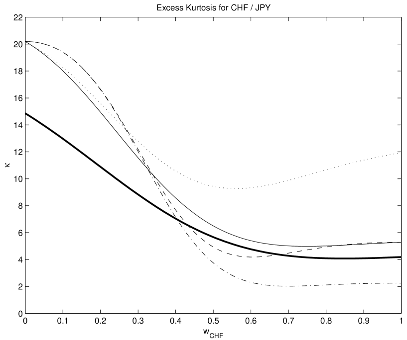
Figure 18: Excess kurtosis of the distribution of the price variation $w_{CHF}x_{CHF}+w_{JPY}x_{JPY}$ of the portfolio made of a fraction $w_{CHF}$ of Swiss franc and a fraction $w_{JPY}=1-w_{CHF}$ of the Japanese Yen against the US dollar, as a function of $w_{CHF}$. Thick solid line : empirical curve, thin solid line : theoretical curve, dashed line : theoretical curve with $\rho=0$ (instead of $\rho=0.43$), dotted line: theoretical curve with $q_{CHF}=2$ rather than $1.75$ and dashed-dotted line: theoretical curve with $q_{CHF}=1.5$. The excess kurtosis has been evaluated for the time interval from Jan. 1971 to Oct. 1998.

Figure 18 plots the excess kurtosis of the sum $w_{CHF}x_{CHF}+w_{JPY}x_{JPY}$ as a function of $w_{CHF}$, with the constraint $w_{CHF}+w_{JPY}=1$. The thick solid line is determined empirically, by direct calculation of the kurtosis from the data. The thin solid line is the theoretical prediction using our theoretical formulas with the empirically determined exponents $c$ and characteristic scales $\chi$ given above. While there is a non-negligible difference, the empirical and theoretical excess kurtosis have essentially the same behavior with their minimum reached almost at the same value of $w_{CHF}$.

Three origins of the discrepancy between theory and empirical data can be invoked. First, as already pointed out in the preceding section, the modified Weibull distribution with constant exponent and scale parameters describes accurately only the tail of the empirical distributions while, for small returns, the empirical distributions are close to a Gaussian law. While putting a strong emphasis on large fluctuations, cumulants of order $4$ are still significantly sensitive to the bulk of the distributions. Moreover, the excess kurtosis is normalized by the square second-order cumulant, which is almost exclusively sensitive to the bulk of the distribution. Cumulants of higher order should thus be better described by the modified Weibull distribution. However, a careful comparison between theory and data would then be hindered by the difficulty in estimating reliable empirical cumulants of high order. This estimation problem is often invoked as a criticism against using high-order moments or cumulants. Our approach suggests that this problem can be in large part circumvented by focusing on the estimation of a reasonable parametric expression for the probability density or distribution function of the assets returns. The second possible origin of the discrepancy between theory and data is the existence of a weak asymmetry of the empirical distributions, particularly of the Swiss franc, which has not been taken into account. The figure also suggests that an error in the determination of the exponents $c$ can also contribute to the discrepancy.

In order to investigate the sensitivity with respect to the choice of the parameters $q$ and $\rho$, we have also constructed the dashed line corresponding to the theoretical curve with $\rho=0$ (instead of $\rho=0.43$) and the dotted line corresponding to the theoretical curve with $q_{CHF}=2$ rather than $1.75$. Finally, the dashed-dotted line corresponds to the theoretical curve with $q_{CHF}=1.5$. We observe that the dashed line remains rather close to the thin solid line while the dotted line departs significantly when $w_{CHF}$ increases. Therefore, the most sensitive parameter is $q$, which is natural because it controls directly the extend of the fat tail of the distributions.

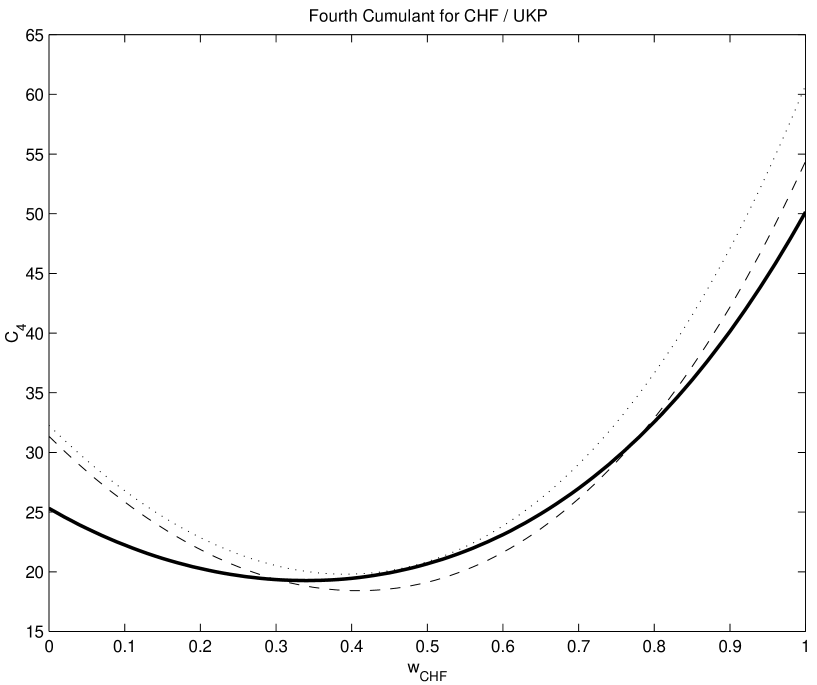
Figure 19: Fourth cumulant for a portfolio made of a fraction $w_{CHF}$ of Swiss Franc and $1-w_{CHF}$ of British Pound. The thick solid line represents the empirical cumulant while the dotted line represents the theoretical cumulant under the symmetric assumption. The dashed line shows the theoretical cumulant when the slight asymmetry of the assets has been taken into account. This cumulant has been evaluated for the time interval from Jan. 1971 to Oct. 1998.

In order to account for the effect of asymmetry, we have plotted the fourth cumulant of a portfolio composed of Swiss Francs and British Pounds. On figure 19, the solid line represents the empirical cumulant while the dashed line shows the theoretical cumulant. The agreement between the two curves is better than under the symmetric asumption. Note once again that an accurate determination of the parameters is the key point to obtain a good agreement between empirical data and theoretical prediction. As we can see in figure 19, the paramaters of the Swiss Franc seem well adjusted since the theoretical and empirical cumulants are both very close when $w_{CHF}\simeq 1$, i.e., when the Swiss Franc is almost the sole asset in the portfolio, while when $w_{CHF}\simeq 0$, the theoretical cumulant is far from the empirical one, i.e., the parameters of the Bristish Pound are not sufficiently well-adjusted.

9 Can you have your cake and eat it too ?

Now that we have shown how to accurately estimate the multivariate distribution fonction of the assets return, let us come back to the portfolio selection problem. In figure 2, we can see that the expected return of the portfolios with minimum risk according to $C_{n}$ decreases when $n$ increases. But, this is not the general situation.

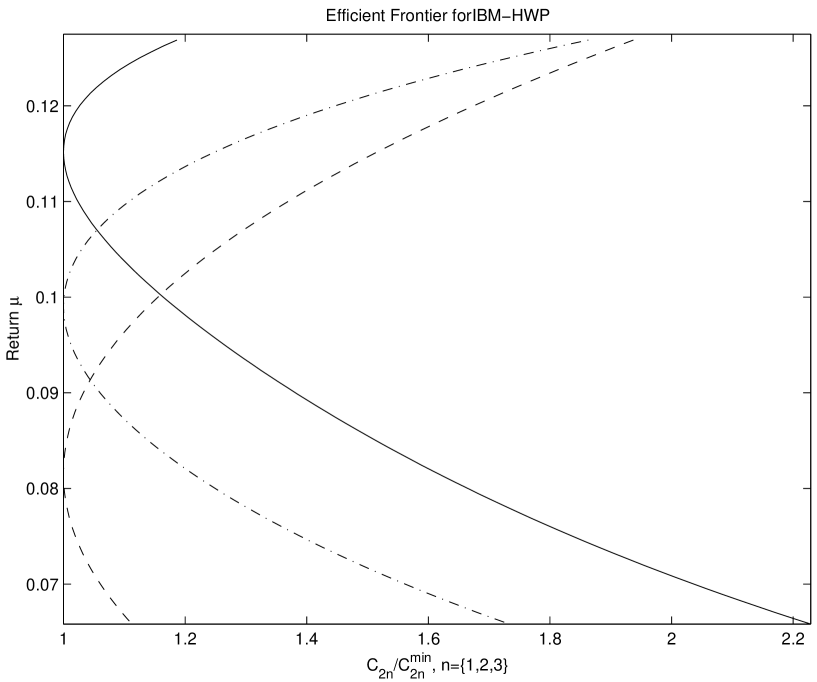
Figure 20: Efficient frontier for a portfolio composed of two stocks: IBM and Hewlett-Packard. The dashed line represents the efficient frontier with respect to the second cumulant, i.e., the standard Markovitz efficient frontier, the dash-dotted line represents the efficient frontier with respect to the fourth cumulant and the solid line is the efficient frontier with respect to the sixth cumulant. The data set used covers the time interval from Jan. 1977 to Dec 2000.

Figure 20 and 21 show the generalized efficient frontiers using $C_{2}$ (Markovitz case), $C_{4}$ or $C_{6}$ as relevant measures of risks, for two portfolios composed of two stocks : IBM and Hewlett-Packard in the first case and IBM and Coca-Cola in the second case.

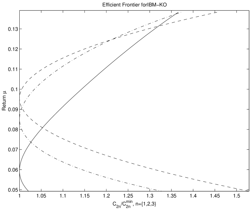
Figure 21: Efficient frontier for a portfolio composed of two stocks: IBM and Coca-Cola. The dashed line represents the efficient frontier with respect to the second cumulant, i.e., the standard Markovitz efficient frontier, the dash-dotted line represents the efficient frontier with respect to the fourth cumulant and the solid line the efficient frontier with repect to the sixth cumulant. The data set used covers the time interval from Jan. 1970 to Dec 2000.

Obviously, given a certain amount of risk, the mean return of the portfolio changes when the cumulant considered changes. It is interesting to note that, in figure 20, the minimisation of large risks, i.e., with respect to $C_{6}$, increases the average return while, in figure 21, the minimisation of large risks lead to decrease the average return.

This allows us to make precise and quantitative the previously reported empirical observation that it is possible to “have your cake and eat it too” [Andersen and Sornette (2001)]. We can indeed give a general criterion to determine under which values of the parameters (exponents $c$ and characteristic scales $\chi$ of the distributions of the asset returns) the average return of the portfolio may increase while the large risks decrease at the same time, thus allowing one to gain on both account (of course, the small risks quantified by the variance will then increase). For two independent assets, assuming that the cumulants of order $n$ and $n+k$ of the portfolio admit a minimum in the interval $]0,1[$, we can show that

$$\mu_{n}^{*}<\mu_{n+k}^{*}$$ (86)

if and only if

$$\left(\mu(1)-\mu(2)\right)~{}\cdot~{}\left[\left(\frac{C_{n}(1)}{C_{n}(2)}\right)^{\frac{1}{n-1}}-\left(\frac{C_{n+k}(1)}{C_{n+k}(2)}\right)^{\frac{1}{n+k-1}}\right]>0~{},$$ (87)

where $\mu_{n}^{*}$ denotes the return of the portfolio evaluated with respect to the minimum of the cumulant of order $n$ and $C_{n}(i)$ is the cumulant of order $n$ for the asset $i$.

The proof of this result and its generalisation to $N>2$ are given in appendix F. In fact, we have observed that when the exponent $c$ of the assets remains sufficiently different, this result still holds in presence of dependence between assets. This last empirical observation in the presence of dependence between assets has not been proved mathematically. It seems reasonable for assets with moderate dependence while it may fail when the dependence becomes too strong as occurs for comonotonic assets.

For the assets considered above, we have found $\mu_{IBM}=0.13$, $\mu_{HWP}=0.07$, $\mu_{KO}=0.05$ and

$$\frac{C_{2}(IBM)}{C_{2}(HWP)} =1.76>\left(\frac{C_{4}(IBM)}{C_{4}(HWP)}\right)^{\frac{1}{3}} =1.03>\left(\frac{C_{6}(IBM)}{C_{6}(HWP)}\right)^{\frac{1}{5}}=0.89$$ (88)

$$\frac{C_{2}(IBM)}{C_{2}(KO)} =0.96<\left(\frac{C_{4}(IBM)}{C_{4}(KO)}\right)^{\frac{1}{3}} =1.01<\left(\frac{C_{6}(IBM)}{C_{6}(KO)}\right)^{\frac{1}{5}}=1.06~{},$$ (89)

which shows that, for the portfolio IBM / Hewlett-Packard, the efficient return is an increasing function of the order of the cumulants while, for the portfolio IBM / Coca-Cola, the inverse phenomenon occurs. This is exactly what is shown on figures 20 and 21.

The underlying intuitive mechanism is the following: if a portfolio contains an asset with a rather fat tail (many “large” risks) but narrow waist (few “small” risks) with very little return to gain from it, minimizing the variance $C_{2}$ of the return portfolio will overweight this asset which is wrongly perceived as having little risk due to its small variance (small waist). In contrast, controlling for the larger risks quantified by $C_{4}$ or $C_{6}$ leads to decrease the weight of this asset in the portfolio, and correspondingly to increase the weight of the more profitable assets. We thus see that the effect of “both decreasing large risks and increasing profit” appears when the asset(s) with the fatter tails, and therefore the narrower central part, has(ve) the smaller overall return(s). A mean-variance approach will weight them more than deemed appropriate from a prudential consideration of large risks and consideration of profits.

From a behavioral point of view, this phenomenon is very interesting and can probably be linked with the fact that the main risk measure considered by the agents is the volatility (or the variance), so that the other dimensions of the risk, measured by higher moments, are often neglected. This may sometimes offer the opportunity of increasing the expected return while lowering large risks.

10 Conclusion

We have introduced three axioms that define a consistent set of risk measures, in the spirit of [Artzner et al. (1997), Artzner et al. (1999)]. Contrarily to the risk measures of [Artzner et al. (1997), Artzner et al. (1999)], our consistent risk measures may account for both-side risks and not only for down-side risks. Thus, they supplement the notion of coherent measures of risk and are well adapted to the problem of portfolio risk assessment and optimization. We have shown that these risk measures, which contain centered moments (and cumulants with some restriction) as particular examples, generalize them significantly. We have presented a generalization of previous generalizations of the efficient frontiers and of the CAPM based on these risk measures in the cases of homogeneous and heterogeneous agents. We have then proposed a simple but powerful specific von Mises representation of multivariate distribution of returns that allowed us to obtain new analytical results on and empirical tests of a general framework for a portfolio theory of non-Gaussian risks with non-linear correlations. Quantitative tests have been presented on a basket of seventeen stocks among the largest capitalization on the NYSE.

This work opens several novel interesting avenues for research. One consists in extending the Gaussian copula assumption, for instance by using the maximum-entropy principle with non-extensive Tsallis entropies, known to be the correct mathematical information-theoretical representation of power laws. A second line of research would be to extend the present framework to encompass simultaneously different time scales $\tau$ in the spirit of [Muzy et al. (2001)] in the case of a cascade model of volatilities.

Appendix A Description of the data set

We have considered a set of seventeen assets traded on the New York Stock Exchange: Applied Material, Coca-Cola, EMC, Exxon-Mobil, General Electric, General Motors, Hewlett Packard, IBM, Intel, MCI WorldCom, Medtronic, Merck, Pfizer, Procter & Gambel, SBC Communication, Texas Instrument, Wall Mart. These assets have been choosen since they are among the largest capitalizations of the NYSE at the time of writing.

The dataset comes from the Center for Research in Security Prices (CRSP) database and covers the time interval from the end of January 1995 to the end of December 2000, which represents exactly 1500 trading days. The main statistical features of the compagnies composing the dataset are presented in the table 5. Note the high kurtosis of each distribution of returns as well as the large values of the observed minimum and maximum returns compared with the standard deviations, that clearly underlines the non-Gaussian behavior of these assets.

Appendix B Generalized efficient frontier and two funds separation theorem

Let us consider a set of $N$ risky assets $X_{1},\cdots,X_{N}$ and a risk-free asset $X_{0}$. The problem is to find the optimal allocation of these assets in the following sense:

$$\left\{\begin{array}[]{l}\inf_{w_{i}\in[0,1]}\rho_{\alpha}(\{w_{i}\})\\ \sum_{i\geq 0}w_{i}=1\\ \sum_{i\geq 0}w_{i}\mu(i)=\mu~{},\end{array}\right.$$ (90)

In other words, we search for the portfolio ${\cal P}$ with minimum risk as measured by any risk measure $\rho_{\alpha}$ obeying axioms I-IV of section 2 for a given amount of expected return $\mu$ and normalized weights $w_{i}$. Short-sells are forbidden except for the risk-free asset which can be lent and borrowed at the same interest rate $\mu_{0}$. Thus, the weights $w_{i}$’s are assumed positive for all $i\geq 1$.

B.1 Case of independent assets when the risk is measured by the cumulants

To start with a simple example, let us assume that the risky assets are independent and that we choose to measure the risk with the cumulants of their distributions of returns. The case when the assets are dependent and/or when the risk is measured by any $\rho_{\alpha}$ will be considered later. Since the assets are assumed independent, the cumulant of order $n$ of the pdf of returns of the portfolio is simply given by

$$C_{n}=\sum_{i=1}^{N}{w_{i}}^{n}~{}C_{n}(i),$$ (91)

where $C_{n}(i)$ denotes the marginal n^th order cumulant of the pdf of returns of the asset $i$. In order to solve this problem, let us introduce the Lagrangian

$${\cal L}=C_{n}-{\lambda_{1}}\left(\sum_{i=0}^{N}w_{i}~{}\mu(i)-\mu\right)-\lambda_{2}\left(\sum_{i=0}^{N}w_{i}-1\right),$$ (92)

where ${\lambda_{1}}$ and $\lambda_{2}$ are two Lagrange multipliers. Differentiating with respect to $w_{0}$ yields

$$\lambda_{2}=\mu_{0}~{}{\lambda_{1}},$$ (93)

which by substitution in equation (92) gives

$${\cal L}=C_{n}-\lambda_{1}\left(\sum_{i=1}^{N}w_{i}~{}(\mu(i)-\mu_{0})-(\mu-\mu_{0})\right).$$ (94)

Let us now differentiate ${\cal L}$ with respect to $w_{i}$, $i\geq 1$, we obtain

$$n~{}{w_{i}^{*}}^{n-1}~{}C_{n}(i)-\lambda_{1}(\mu(i)-\mu_{0})=0,$$ (95)

so that

$${w_{i}^{*}}={\lambda_{1}}^{\frac{1}{n-1}}~{}\left(\frac{\mu(i)-\mu_{0}}{n~{}C_{n}(i)}\right)^{\frac{1}{n-1}}.$$ (96)

Applying the normalization constraint yields

$$w_{0}+{\lambda_{1}}^{\frac{1}{n-1}}~{}\sum_{i=1}^{N}\left(\frac{\mu(i)-\mu_{0}}{n~{}C_{n}(i)}\right)^{\frac{1}{n-1}}=1,$$ (97)

thus

$${\lambda_{1}}^{\frac{1}{n-1}}=\frac{1-w_{0}}{\sum_{i=1}^{N}\left(\frac{\mu(i)-\mu_{0}}{n~{}C_{n}(i)}\right)^{\frac{1}{n-1}}},$$ (98)

and finally

$$w_{i}^{*}=(1-w_{0})~{}\frac{\left(\frac{\mu(i)-\mu_{0}}{C_{n}(i)}\right)^{\frac{1}{n-1}}}{\sum_{i=1}^{N}\left(\frac{\mu(i)-\mu_{0}}{C_{n}(i)}\right)^{\frac{1}{n-1}}}.$$ (99)

Let us now define the portfolio $\Pi$ exclusively made of risky assets with weights

$$\tilde{w}_{i}=\frac{\left(\frac{\mu(i)-\mu_{0}}{C_{n}(i)}\right)^{\frac{1}{n-1}}}{\sum_{i=1}^{N}\left(\frac{\mu(i)-\mu_{0}}{C_{n}(i)}\right)^{\frac{1}{n-1}}},~{}~{}~{}~{}~{}~{}~{}i\geq 1.$$ (100)

The optimal portfolio ${\cal P}$ can be split in two funds : the risk-free asset whose weight is $w_{0}$ and a risky fund $\Pi$ with weight $(1-w_{0})$. The expected return of the portfolio ${\cal P}$ is thus

$$\mu=w_{0}~{}\mu_{0}+(1-w_{0})\mu_{\Pi},$$ (101)

where $\mu_{\Pi}$ denotes the expected return of portofolio $\Pi$:

$$\mu_{\Pi}=\frac{\sum_{i=1}^{N}\mu(i)~{}\left(\frac{\mu(i)-\mu_{0}}{C_{n}(i)}\right)^{\frac{1}{n-1}}}{\sum_{i=1}^{N}\left(\frac{\mu(i)-\mu_{0}}{C_{n}(i)}\right)^{\frac{1}{n-1}}}.$$ (102)

The risk associated with ${\cal P}$ and measured by the cumulant $C_{n}$ of order $n$ is

$$C_{n}=(1-w_{0})^{n}~{}\frac{\sum_{i=1}^{N}C_{n}(i)~{}\left(\frac{\mu(i)-\mu_{0}}{C_{n}(i)}\right)^{\frac{n}{n-1}}}{\left[\sum_{i=1}^{N}\left(\frac{\mu(i)-\mu_{0}}{C_{n}(i)}\right)^{\frac{1}{n-1}}\right]^{n}}~{}.$$ (103)

Putting together the three last equations allows us to obtain the equation of the efficient frontier:

$$\mu=\mu_{0}+\left[\sum\frac{(\mu(i)-\mu_{0})^{\frac{n}{n-1}}}{C_{n}(i)^{\frac{1}{n-1}}}\right]^{\frac{n-1}{n}}\cdot{C_{n}}^{\frac{1}{n}},$$ (104)

which is a straight line in the plane ${(C_{n}}^{1/n},~{}\mu)$.

B.2 General case

Let us now consider the more realistic case when the risky assets are dependent and/or when the risk is measured by any risk measure $\rho_{\alpha}$ obeying the axioms I-IV presented in section 2, where $\alpha$ denotes the degres of homogeneity of $\rho_{\alpha}$. Equation (94) always holds (with $C_{n}$ replaced by $\rho_{\alpha}$), and the differentiation with respect to $w_{i}$, $i\geq 1$ yields the set of equations:

$$\frac{\partial\rho_{\alpha}}{\partial w_{i}}(w_{1}^{*},\cdots,w_{N}^{*})=\lambda_{1}~{}(\mu(i)-\mu_{0}),~{}~{}~{}~{}~{}~{}~{}i\in\{1,\cdots,N\}.$$ (105)

Since $\rho_{\alpha}(w_{1},\cdots,w_{N})$ is a homogeneous function of order $\alpha$, its first-order derivative with respect to $w_{i}$ is also a homogeneous function of order $\alpha-1$. Using this homogeneity property allows us to write

$${\lambda_{1}}^{-1}~{}\frac{\partial\rho_{\alpha}}{\partial w_{i}}(w_{1}^{*},\cdots,w_{N}^{*}) = (\mu(i)-\mu_{0}),~{}~{}~{}~{}~{}~{}~{}i\in\{1,\cdots,N\},$$ (106)

$$\frac{\partial\rho_{\alpha}}{\partial w_{i}}\left({\lambda_{1}}^{-\frac{1}{\alpha-1}}w_{1}^{*},\cdots,{\lambda_{1}}^{-\frac{1}{\alpha-1}}w_{N}^{*}\right) = (\mu(i)-\mu_{0}),~{}~{}~{}~{}~{}~{}~{}i\in\{1,\cdots,N\}~{}.$$ (107)

Denoting by $\{\hat{w}_{1},\cdots,\hat{w}_{N}\}$ the solution of

$$\frac{\partial\rho_{\alpha}}{\partial w_{i}}(\hat{w}_{1},\cdots,\hat{w}_{N})=(\mu(i)-\mu_{0}),~{}~{}~{}~{}~{}~{}~{}i\in\{1,\cdots,N\},$$ (108)

this shows that the optimal weights are

$$w_{i}^{*}={\lambda_{1}}^{\frac{1}{\alpha-1}}\hat{w}_{i}.$$ (109)

Now, performing the same calculation as in the case of independent risky assets, the efficient portfolio ${\cal P}$ can be realized by investing a weight $w_{0}$ of the initial wealth in the risk-free asset and the weight $(1-w_{0})$ in the risky fund $\Pi$, whose weights are given by

$$\tilde{w}_{i}=\frac{\hat{w}_{i}}{\sum_{i=1}^{N}\hat{w}_{i}}~{}.$$ (110)

Therefore, the expected return of every efficient portfolio is

$$\mu=w_{0}\cdot\mu_{0}+(1-w_{0})\cdot\mu_{\Pi},$$ (111)

where $\mu_{\Pi}$ denotes the expected return of the market portfolio $\Pi$, while the risk, measured by $\rho_{\alpha}$ is

$$\rho_{\alpha}=(1-w_{0})^{\alpha}\rho_{\alpha}(\Pi)~{},$$ (112)

so that

$$\mu=\mu_{0}+\frac{\mu_{\Pi}-\mu_{0}}{{\rho_{\alpha}(\Pi)}^{1/\alpha}}~{}{\rho_{\alpha}}^{1/\alpha}~{}.$$ (113)

This expression is the natural generalization of the relation obtained by [Markovitz (1959)] for mean-variance efficient portfolios.

Appendix C Composition of the market portfolio

In this appendix, we derive the relationship between the composition of the market portfolio and the composition of the optimal portfolio $\Pi$ obtained by the minimization of the risks measured by $\rho_{\alpha}(n)$.

C.1 Homogeneous case

We first consider a homogeneous market, peopled with agents choosing their optimal portfolio with respect to the same risk measure $\rho_{\alpha}$. A given agent $p$ invests a fraction $w_{0}(p)$ of his wealth $W(p)$ in the risk-free asset and a fraction $1-w_{0}(p)$ in the optimal portfolio $\Pi$. Therefore, the total demand $D_{i}$ of asset $i$ is the sum of the demand $D_{i}(p)$ over all agents $p$ in asset $i$:

$$D_{i} = \sum_{p}D_{i}(p)~{},$$ (114)

$$= \sum_{p}W(p)\cdot(1-w_{0}(p))\cdot\tilde{w}_{i}~{},$$ (115)

$$= \tilde{w}_{i}\cdot\sum_{p}W(p)\cdot(1-w_{0}(p))~{},$$ (116)

where the $\tilde{w}_{i}$’s are given by (110). The aggregated demand $D$ over all assets is

$$D = \sum_{i}D_{i},$$ (117)

$$= \sum_{i}\tilde{w}_{i}\cdot\sum_{p}W(p)\cdot(1-w_{0}(p)),$$ (118)

$$= \sum_{p}W(p)\cdot(1-w_{0}(p)).$$ (119)

By definition, the weight of asset $i$, denoted by $w_{i}^{m}$, in the market portfolio equals the ratio of its capitalization (the supply $S_{i}$ of asset $i$) over the total capitalization of the market $S=\sum S_{i}$. At the equilibrium, demand equals supply, so that

$$w_{i}^{m}=\frac{S_{i}}{S}=\frac{D_{i}}{D}=\tilde{w}_{i}.$$ (121)

Thus, at the equilibrium, the optimal portfolio $\Pi$ is the market portfolio.

C.2 Heterogeneous case

We now consider a heterogenous market, defined such that the agents choose their optimal portfolio with respect to different risk measures. Some of them choose the usual mean-variance optimal portfolios, others prefer any mean-$\rho_{\alpha}$ efficient portfolio, and so on. Let us denote by $\Pi_{n}$ the mean-$\rho_{\alpha}(n)$ optimal portfolio made only of risky assets. Let $\phi_{n}$ be the fraction of agents who choose the mean-$\rho_{\alpha}(n)$ efficient portfolios. By normalization, $\sum_{n}\phi_{n}=1$. The demand $D_{i}(n)$ of asset $i$ from the agents optimizing with respect to $\rho_{\alpha}(n)$ is

$$D_{i}(n) = \sum_{p\in{\cal S}_{n}}W(p)\cdot(1-w_{0}(p))\cdot\tilde{w}_{i}(n),$$ (122)

$$= \tilde{w}_{i}(n)\sum_{p\in{\cal S}_{n}}W(p)\cdot(1-w_{0}(p)),$$ (123)

where ${\cal S}_{n}$ denotes the set of agents, among all the agents, who follow the optimization stragtegy with respect to $\rho_{\alpha}(n)$. Thus, the total demand of asset $i$ is

$$D_{i} = \sum_{n}{\cal N}\phi_{n}\cdot D_{i}(n),$$ (124)

$$= {\cal N}\sum_{n}\phi_{n}\cdot\tilde{w}_{i}(n)\sum_{p\in{\cal S}_{n}}W(p)\cdot(1-w_{0}(p)),$$ (125)

where ${\cal N}$ is the total number of agents. This finally yields the total demand $D$ for all assets and for all agents

$$D = \sum_{i}D_{i},$$ (126)

$$= {\cal N}\sum_{i}\sum_{n}\phi_{n}\cdot\tilde{w}_{i}(n)\sum_{p\in{\cal S}_{n}}W(p)\cdot(1-w_{0}(p)),$$ (127)

$$= {\cal N}\sum_{n}\phi_{n}\sum_{p\in{\cal S}_{n}}W(p)\cdot(1-w_{0}(p)),$$ (128)

since $\sum_{i}\tilde{w}_{i}(n)=1$, for every $n$. Thus, setting

$$\gamma_{n}=\frac{\phi_{n}\sum_{p\in{\cal S}_{n}}W(p)\cdot(1-w_{0}(p))}{\sum_{n}\phi_{n}\sum_{p\in{\cal S}_{n}}W(p)\cdot(1-w_{0}(p))}~{},$$ (129)

the market portfolio is the weighted sum of the mean-$\rho_{\alpha}(n)$ optimal portfolios $\Pi_{n}$:

$$w_{i}^{m}=\frac{S_{i}}{S}=\frac{D_{i}}{D}=\sum_{n}\gamma_{n}\cdot\tilde{w}_{i}(n)~{}.$$ (130)

Appendix D Generalized capital asset princing model

Our proof of the generalized capital asset princing model is similar to the usual demontration of the CAPM.

Let us consider an efficient portfolio ${\cal P}$. It necessarily satisfies equation (105) in appendix B :

$$\frac{\partial\rho_{\alpha}}{\partial w_{i}}(w_{1}^{*},\cdots,w_{N}^{*})=\lambda_{1}~{}(\mu(i)-\mu_{0}),~{}~{}~{}~{}~{}~{}~{}i\in\{1,\cdots,N\}.$$ (131)

Let us now choose any portfolio ${\cal R}$ made only of risky assets and let us denote by $w_{i}({\cal R})$ its weights. We can thus write

$$\sum_{i=1}^{N}w_{i}({\cal R})\cdot\frac{\partial\rho_{\alpha}}{\partial w_{i}}(w_{1}^{*},\cdots,w_{N}^{*}) = \lambda_{1}~{}\sum_{i=1}^{N}w_{i}({\cal R})\cdot(\mu(i)-\mu_{0}),$$ (132)

$$= \lambda_{1}~{}(\mu_{\cal R}-\mu_{0}).$$ (133)

We can apply this last relation to the market portfolio $\Pi$, because it is only composed of risky assets (as proved in appendix B). This leads to $w_{i}({\cal R})=w_{i}^{*}$ and $\mu_{\cal R}=\mu_{\Pi}$, so that

$$\sum_{i=1}^{N}w_{i}^{*}\cdot\frac{\partial\rho_{\alpha}}{\partial w_{i}}(w_{1}^{*},\cdots,w_{N}^{*})=\lambda_{1}~{}(\mu_{\Pi}-\mu_{0}),$$ (134)

which, by the homogeneity of the risk measures $\rho_{\alpha}$, yields

$$\alpha\cdot\rho_{\alpha}(w_{1}^{*},\cdots,w_{N}^{*})=\lambda_{1}~{}(\mu_{\Pi}-\mu_{0})~{}.$$ (135)

Substituting equation (131) into (135) allows us to obtain

$$\mu_{j}-\mu_{0}=\beta_{\alpha}^{j}\cdot(\mu_{\Pi}-\mu_{0}),$$ (136)

where

$$\beta_{\alpha}^{j}=\frac{\partial\left(\ln{\rho_{\alpha}}^{\frac{1}{\alpha}}\right)}{\partial w_{j}}~{},$$ (137)

calculated at the point $\{w_{1}^{*},\cdots,w_{N}^{*}\}$. Expression (135) with (137) provides our CAPM, generalized with respect to the risk measures $\rho_{\alpha}$.

In the case where $\rho_{\alpha}$ denotes the variance, the second-order centered moment is equal to the second-order cumulant and reads

$$C_{2} = w_{1}^{*}\cdot{\rm Var}[X_{1}]+2w_{1}^{*}w_{2}^{*}\cdot{\rm Cov}(X_{1},X_{2})+w_{2}^{*}\cdot{\rm Var}[X_{2}],$$ (138)

$$= {\rm Var}[\Pi]~{}.$$ (139)

Since

$$\frac{1}{2}\cdot\frac{\partial C_{2}}{\partial w_{1}} = w_{1}^{*}\cdot{\rm Var}[X_{1}]+w_{2}^{*}\cdot{\rm Cov}(X_{1},X_{2})~{},$$ (140)

$$= {\rm Cov}(X_{1},\Pi),$$ (141)

we find

$$\beta=\frac{{\rm Cov}(X_{1},X_{\Pi})}{{\rm Var}[X_{\Pi}]}~{},$$ (142)

which is the standard result of the CAPM derived from the mean-variance theory.

Appendix E Calculation of the moments of the distribution of portfolio returns

Let us start with equation (72) in the $2$-asset case :

$$\hat{P}_{S}(k)=\frac{1}{2\pi\sqrt{1-\rho^{2}}}\int dy_{1}dy_{2}~{}exp\left[-\frac{1}{2}y^{t}V^{-1}y+ik\left(\chi_{1}w_{1}sgn(y_{1})\left|\frac{y_{1}}{\sqrt{2}}\right|^{q_{1}}+\right.\right.{}$$

$$\left.\left.+\chi_{2}w_{2}sgn(y_{2})\left|\frac{y_{2}}{\sqrt{2}}\right|^{q_{2}}\right)\right]\;.$$ (143)

Expanding the exponential and using the definition (67) of moments, we get

$$M_{n}=\frac{1}{2\pi\sqrt{1-\rho^{2}}}\int dy_{1}\int dy_{2}\sum_{p=0}^{n}{n\choose p}\chi_{1}^{p}\chi_{2}^{n-p}w_{1}^{p}w_{2}^{n-p}sgn(y_{1})^{p}\left|\frac{y_{1}}{\sqrt{2}}\right|^{q_{1}p}\times$$

$$\times sgn(y_{2})^{n-p}\left|\frac{y_{2}}{\sqrt{2}}\right|^{q_{2}(n-p)}\,e^{-\frac{1}{2}y^{t}V^{-1}y}\;.$$ (144)

Posing

$$\gamma_{q_{1}q_{2}}(n,p)=\frac{{\chi_{1}}^{p}{\chi_{2}}^{n-p}}{2\pi\sqrt{1-\rho^{2}}}\int dy_{1}dy_{2}\;sgn(y_{1})^{p}\left|\frac{y_{1}}{\sqrt{2}}\right|^{q_{1}p}sgn(y_{2})^{n-p}\left|\frac{y_{2}}{\sqrt{2}}\right|^{q_{2}(n-p)}\,e^{-\frac{1}{2}y^{t}V^{-1}y}\;,$$ (145)

this leads to

$$M_{n}=\sum_{p=0}^{n}{n\choose p}w_{1}^{p}w_{2}^{n-p}\gamma_{q_{1}q_{2}}(n,p)\;.$$ (146)

Let us defined the auxiliary variables $\alpha$ and $\beta$ such that

$$\left\{\begin{array}[]{rlc}\alpha&=&(V^{-1})_{11}=(V^{-1})_{22}=\frac{1}{1-\rho^{2}}\;,\\ \beta&=&-(V^{-1})_{12}=-(V^{-1})_{21}=\frac{\rho}{1-\rho^{2}}\;.\end{array}\right.$$ (147)

Performing a simple change of variable in (145), we can transform the integration such that it is defined solely within the first quadrant ($y_{1}\geq 0$, $y_{2}\geq 0$), namely

$$\gamma_{q_{1}q_{2}}(n,p)={\chi_{1}}^{p}{\chi_{2}}^{n-p}\frac{1+(-1)^{n}}{2\pi\sqrt{1-\rho^{2}}}\int_{0}^{+\infty}dy_{1}\int_{0}^{+\infty}dy_{2}~{}\left(\frac{y_{1}}{\sqrt{2}}\right)^{q_{1}p}\left(\frac{y_{2}}{\sqrt{2}}\right)^{q_{2}(n-p)}\,e^{-\frac{\alpha}{2}(y_{1}^{2}+y_{2}^{2})}\times$$

$$\times\left(e^{\beta y_{1}y_{2}}+(-1)^{p}e^{-\beta y_{1}y_{2}}\right)\;.$$ (148)

This equation imposes that the coefficients $\gamma$ vanish if $n$ is odd. This leads to the vanishing of the moments of odd orders, as expected for a symmetric distribution. Then, we expand $e^{\beta y_{1}y_{2}}+(-1)^{p}e^{-\beta y_{1}y_{2}}$ in series. Permuting the sum sign and the integral allows us to decouple the integrations over the two variables $y_{1}$ and $y_{2}$:

$$\gamma_{q_{1}q_{2}}(n,p)={\chi_{1}}^{p}{\chi_{2}}^{n-p}\frac{1+(-1)^{n}}{2\pi\sqrt{1-\rho^{2}}}\sum_{s=0}^{+\infty}[1+(-1)^{p+s}]\frac{\beta^{s}}{s!}\left(\int_{0}^{+\infty}dy_{1}~{}\frac{y_{1}^{q_{1}p+s}}{2^{\frac{q_{1}p}{2}}}~{}e^{-\frac{\alpha}{2}y_{1}^{2}}\right)\times$$

$$\times\left(\int_{0}^{+\infty}dy_{2}~{}\frac{y_{2}^{q_{2}(n-p)+s}}{2^{\frac{q_{2}(n-p)}{2}}}~{}e^{-\frac{\alpha}{2}y_{1}^{2}}\right)\;.$$ (149)

This brings us back to the problem of calculating the same type of integrals as in the uncorrelated case. Using the expressions of $\alpha$ and $\beta$, and taking into account the parity of $n$ and $p$, we obtain:

$$\gamma_{q_{1}q_{2}}(2n,2p) = {\chi_{1}}^{2p}{\chi_{2}}^{2n-2p}\frac{(1-\rho^{2})^{q_{1}p+q_{2}(n-p)+\frac{1}{2}}}{\pi}\sum_{s=0}^{+\infty}\frac{(2\rho)^{2s}}{(2s)!}\Gamma\left(q_{1}p+s+\frac{1}{2}\right)\times$$ (150)

$$\times\Gamma\left(q_{2}(n-p)+s+\frac{1}{2}\right)\;,$$

$$\gamma_{q_{1}q_{2}}(2n,2p+1) = {\chi_{1}}^{2p+1}{\chi_{2}}^{2n-2p-1}\frac{(1-\rho^{2})^{q_{1}p+q_{2}(n-p)+\frac{q_{1}-q_{2}+1}{2}}}{\pi}\sum_{s=0}^{+\infty}\frac{(2\rho)^{2s+1}}{(2s+1)!}\times$$ (151)

$$\times\Gamma\left(q_{1}p+s+1+\frac{q_{1}}{2}\right)\Gamma\left(q_{2}(n-p)+s+1-\frac{q_{2}}{2}\right)\;.$$

Using the definition of the hypergeometric functions ${}_{2}F_{1}$ [Abramovitz and Stegun (1972)], and the relation (9.131) of [Gradshteyn and Ryzhik (1965)], we finally obtain

$$\gamma_{q_{1}q_{2}}(2n,2p) = {\chi_{1}}^{2p}{\chi_{2}}^{2n-2p}\frac{\Gamma\left(q_{1}p+\frac{1}{2}\right)\Gamma\left(q_{2}(n-p)+\frac{1}{2}\right)}{\pi}~{}{{}_{2}F_{1}}\left(-q_{1}p,-q_{2}(n-p);\frac{1}{2};\rho^{2}\right)\;,$$ (152)

$$\gamma_{q_{1}q_{2}}(2n,2p+1) = {\chi_{1}}^{2p+1}{\chi_{2}}^{2n-2p-1}\frac{2\Gamma\left(q_{1}p+1+\frac{q_{1}}{2}\right)\Gamma\left(q_{2}(n-p)+1-\frac{q_{2}}{2}\right)}{\pi}\rho~{}\times$$ (153)

$$\times~{}{{}_{2}F_{1}}\left(-q_{1}p-\frac{q_{1}-1}{2},-q_{2}(n-p)+\frac{q_{2}+1}{2};\frac{3}{2};\rho^{2}\right)\;.$$

In the asymmetric case, a similar calculation follows, with the sole difference that the results involves four terms in the integral (E) instead of two.

Appendix F Conditions under which it is possible to increase the return and decrease large risks simultaneously

We consider $N$ independent assets $\{1\cdots N\}$, whose returns are denoted by $\mu(1)\cdots\mu(N)$. We aggregate these assets in a portfolio. Let $w_{1}\cdots w_{N}$ be their weights. We consider that short positions are forbidden and that $\sum_{i}w_{i}=1$. The return $\mu$ of the portfolio is

$$\mu=\sum_{i=1}^{N}w_{i}\mu(i).$$ (154)

The risk of the portfolio is quantified by the cumulants of the distribution of $\mu$.

Let us denote $\mu_{n}^{*}$ the return of the portfolio evaluated for the asset weights which minimize the cumulant of order $n$.

F.1 Case of two assets

Let $C_{n}$ be the cumulant of order n for the portfolio. The assets being independent, we have

$$C_{n} = C_{n}(1){w_{1}}^{n}+C_{n}(2){w_{2}}^{n},$$ (155)

$$= C_{n}(1){w_{1}}^{n}+C_{n}(2)(1-w_{1})^{n}.$$ (156)

In the following, we will drop the subscript $1$ in $w_{1}$, and only write $w$. Let us evaluate the value $w=w^{*}$ at the minimum of $C_{n}$, $n>2$ :

$$\frac{dC_{n}}{dw}=0 \Longleftrightarrow C_{n}(1)w^{n-1}-C_{n}(2)(1-w)^{n-1}=0,$$ (157)

$$\Longleftrightarrow \frac{C_{n}(1)}{C_{n}(2)}=\left(\frac{1-w^{*}}{w^{*}}\right)^{n-1},$$ (158)

and assuming that $C_{n}(1)/C_{n}(2)>0$, which is satisfied according to our positivity axiom 1, we obtain

$$w^{*}=\frac{C_{n}(2)^{\frac{1}{n-1}}}{C_{n}(1)^{\frac{1}{n-1}}+C_{n}(2)^{\frac{1}{n-1}}}.$$ (159)

This leads to the following expression for $\mu_{n}^{*}$ :

$$\mu_{n}^{*}=\frac{\mu(1)\cdot C_{n}(2)^{\frac{1}{n-1}}+\mu(2)\cdot C_{n}(1)^{\frac{1}{n-1}}}{C_{n}(1)^{\frac{1}{n-1}}+C_{n}(2)^{\frac{1}{n-1}}}.$$ (160)

Thus, after simple algebraic manipulations, we find

$$\mu_{n}^{*}<\mu_{n+k}^{*}\Longleftrightarrow(\mu(1)-\mu(2))\left(C_{n}(1)^{\frac{1}{n-1}}C_{n+k}(2)^{\frac{1}{n+k-1}}-C_{n}(2)^{\frac{1}{n-1}}C_{n+k}(1)^{\frac{1}{n+k-1}}\right)>0,$$ (161)

which concludes the proof of the result announced in the main body of the text.

F.2 General case

We now consider a portfolio with $N$ independent assets. Assuming that the cumulants $C_{n}(i)$ have the same sign for all $i$ (according to axiom 1), we are going to show that the minimum of $C_{n}$ is obtained for a portfolio whose weights are given by

$$w_{i}=\frac{\prod_{j\neq i}^{N}C_{n}(j)^{\frac{1}{n-1}}}{\sum_{j=1}^{N}C_{n}(j)^{\frac{1}{n-1}}},$$ (162)

and we have

$$\mu_{n}^{*}=\frac{\sum_{i=1}^{N}\left(\mu(i)\prod_{j\neq i}^{N}C_{n}(j)^{\frac{1}{n-1}}\right)}{\sum_{j=1}^{N}C_{n}(j)^{\frac{1}{n-1}}}~{}.$$ (163)

Indeed, the cumulant of the portfolio is given by

$$C_{n}=\sum_{i=1}^{N}C_{n}(i)~{}w_{i}^{n}$$ (164)

subject to the constraint

$$\sum_{i=1}^{N}w_{i}=1.$$ (165)

Introducing a Lagrange multiplier $\lambda$, the first order conditions yields

$$C_{n}(i)~{}w_{i}^{n-1}-\lambda=0,~{}~{}~{}~{}\forall i\in\{1,\cdots,N\},$$ (166)

so that

$$w_{i}^{n-1}=\frac{\lambda}{C_{n}(i)}.$$ (167)

Since all the $C_{n}(i)$ are positive, we can find a $\lambda$ such that all the $w_{i}$ are real and positive, which yields the announced result (162). From here, there is no simple condition that ensures $\mu_{n}^{*}<\mu_{n+k}^{*}$. The simplest way to compare $\mu_{n}^{*}$ and $\mu_{n+k}^{*}$ is to calculate diretly these quantities using the formula (163).

$\mu$	${\mu_{2}}^{1/2}$	${\mu_{4}}^{1/4}$	${\mu_{6}}^{1/6}$	${\mu_{8}}^{1/8}$
0.10%	0.92%	1.36%	1.79%	2.15%
0.12%	0.96%	1.43%	1.89%	2.28%
0.14%	1.05%	1.56%	2.06%	2.47%
0.16%	1.22%	1.83%	2.42%	2.91%
0.18%	1.47%	2.21%	2.92%	3.55%
0.20%	1.77%	2.65%	3.51%	4.22%

Table 1: This table presents the risk measured by $\mu_{n}^{1/n}$ for n=2,4,6,8, for a given value of the expectedd (daily) return $\mu$.

	$\frac{\mu}{\mu_{2}^{1/2}}$	$\frac{\mu}{\mu_{4}^{1/4}}$	$\frac{\mu}{\mu_{6}^{1/6}}$	$\frac{\mu}{C_{4}^{1/4}}$	$\frac{\mu}{C_{6}^{1/6}}$
Wall Mart	0.0821	0.0555	0.0424	0.0710	0.0557
EMC	0.0801	0.0552	0.0430	0.0730	0.0612
Intel	0.0737	0.0512	0.0397	0.0694	0.0532
Hewlett Packard	0.0724	0.0472	0.0354	0.0575	0.0439
IBM	0.0705	0.0465	0.0346	0.0574	0.0421
Merck	0.0628	0.0415	0.0292	0.0513	0.0331
Procter & Gamble	0.0590	0.0399	0.0314	0.0510	0.0521
General Motors	0.0586	0.0362	0.0247	0.0418	0.0269
SBC Communication	0.0584	0.0386	0.0270	0.0477	0.0302
General Electric	0.0569	0.0334	0.0233	0.0373	0.0258
Applied Material	0.0525	0.0357	0.0269	0.0462	0.0338
MCI WorldCom	0.0441	0.0173	0.0096	0.0176	0.0098
Medtronic	0.0432	0.0278	0.0202	0.0333	0.0237
Coca-Cola	0.0430	0.0278	0.0207	0.0335	0.0252
Exxon-Mobil	0.0410	0.0256	0.0178	0.0299	0.0197
Texas Instrument	0.0324	0.0224	0.0171	0.0301	0.0218
Pfizer	0.0298	0.0184	0.0131	0.0213	0.0148

Table 2: This table presents the values of the generalized Sharpe ratios for the set of seventeen assets listed in the first column. The assets are ranked with respect to their Sharpe ratio, given in the second column. The third and fourth columns give the generalized Sharpe ratio calculated with respect to the fourth and sixth centered moments $\mu_{4}$ and $\mu_{6}$ while the fifth and sixth columns give the generalized Sharpe ratio calculated with respect to the fourth and sixth cumulants $C_{4}$ and $C_{6}$.

	Positive Tail					Negative Tail
	$<\chi_{+}>$	$<c_{+}>$	$\chi_{+}$	$c_{+}$		$<\chi_{-}>$	$<c_{-}>$	$\chi_{-}$	$c_{-}$
CHF	2.45	1.61	2.33	1.26		2.34	1.53	1.72	0.93
DEM	2.09	1.65	1.74	1.03		2.01	1.58	1.45	0.91
JPY	2.10	1.28	1.30	0.76		1.89	1.47	0.99	0.76
MAL	1.00	1.22	1.25	0.41		1.01	1.25	0.44	0.48
POL	1.55	1.02	1.30	0.73		1.60	2.13	1.25	0.62
THA	0.78	0.75	0.75	0.54		0.82	0.73	0.30	0.38
UKP	1.89	1.52	1.38	0.92		2.00	1.41	1.82	1.09

Table 3: Table of the exponents $c$ and the scale parameters $\chi$ for different currencies. The subscript ”+” or ”-” denotes the positive or negative part of the distribution of returns and the terms between brackets refer to parameters estimated in the bulk of the distribution while naked parameters refer to the tails of the distribution.

	Positive Tail					Negative Tail
	$<\chi_{+}>$	$<c_{+}>$	$\chi_{+}$	$c_{+}$		$<\chi_{-}>$	$<c_{-}>$	$\chi_{-}$	$c_{-}$
Applied Material	12.47	1.82	8.75	0.99		11.94	1.66	8.11	0.98
Coca-Cola	5.38	1.88	4.46	1.04		5.06	1.74	2.98	0.78
EMC	13.53	1.63	13.18	1.55		11.44	1.61	3.05	0.57
General Electric	5.21	1.89	1.81	1.28		4.80	1.81	4.31	1.16
General Motors	5.78	1.71	0.63	0.48		5.32	1.89	2.80	0.79
Hewlett Packart	7.51	1.93	4.20	0.84		7.26	1.76	1.66	0.52
IBM	5.46	1.71	3.85	0.87		5.07	1.90	0.18	0.33
Intel	8.93	2.31	2.79	0.64		9.14	1.60	3.56	0.62
MCI WorldCom	9.80	1.74	11.01	1.56		9.09	1.56	2.86	0.58
Medtronic	6.82	1.95	6.09	1.11		6.49	1.54	2.55	0.67
Merck	5.36	1.91	4.56	1.16		5.00	1.73	1.32	0.59
Pfizer	6.41	2.01	5.84	1.27		6.04	1.70	0.26	0.35
Procter & Gambel	4.86	1.83	3.53	0.96		4.55	1.74	2.96	0.82
SBC Communication	5.21	1.97	1.26	0.59		4.89	1.59	1.56	0.60
Texas Instrument	9.06	1.78	4.07	0.72		8.24	1.84	2.18	0.54
Wall Mart	7.41	1.83	5.81	1.01		6.80	1.64	3.75	0.78

Table 4: Table of the exponents $c$ and the scale parameters $\chi$ for different stocks. The subscript ”+” or ”-” denotes the positive or negative part of the distribution and the terms between brackets refer to parameters estimated in the bulk of the distribution while naked parameters refer to the tails of the distribution.

	Mean ($10^{-3}$)	Variance ($10^{-3}$)	Skewness	Kurtosis	min	max
Applied Material	2.11	1.62	0.41	4.68	-14%	21%
Coca-Cola	0.81	0.36	0.13	5.71	-11%	10%
EMC	2.76	1.13	0.23	4.79	-18%	15%
Exxon-Mobil	0.92	0.25	0.30	5.26	-7%	11%
General Electric	1.38	0.30	0.08	4.46	-7%	8%
General Motors	0.64	0.39	0.12	4.35	-11%	8%
Hewlett Packard	1.17	0.81	0.16	6.58	-14%	21%
IBM	1.32	0.54	0.08	8.43	-16%	13%
Intel	1.71	0.85	-0.31	6.88	-22%	14%
MCI WorldCom	0.87	0.85	-0.18	6.88	-20%	13%
Medtronic	1.70	0.55	0.23	5.52	-12%	12%
Merck	1.32	0.35	0.18	5.29	-9%	10%
Pfizer	1.57	0.46	0.01	4.28	-10%	10%
Procter&Gambel	0.90	0.41	-2.57	42.75	-31%	10%
SBC Communication	0.86	0.39	0.06	5.86	-13%	9%
Texas Instrument	2.20	1.23	0.50	5.26	-12%	24%
Wall Mart	1.35	0.52	0.16	4.79	-10%	9%

Table 5: This table presents the main statistical features of the daily returns of the set of seventeen assets studied here over the time interval from the end of January 1995 to the end of December 2000.

Figure 12: Cumulative distribution of $z^{2}={\bf y^{t}V^{-1}y}$ versus the cumulative distribution of the chi-square $\chi^{2}$ with two degrees of freedom for the couple Merk / General Electric, for the time interval from Jan. 1970 to Dec. 2000. This $\chi^{2}$ should not be confused with the characteristic scale used in the definition of the modified Weibull distributions.

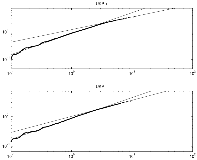
Figure 14: Graph of Gaussianized British Pound returns versus British Pound returns, for the time interval from Jan. 1971 to Oct. 1998. The upper graph gives the positive tail and the lower one the negative tail. The two straight lines represent the curves $y=\sqrt{2}\left(\frac{x}{\langle\chi_{\pm}\rangle}\right)^{\langle c_{\pm}\rangle}$ and $y=\sqrt{2}\left(\frac{x}{\chi_{\pm}}\right)^{c_{\pm}}$

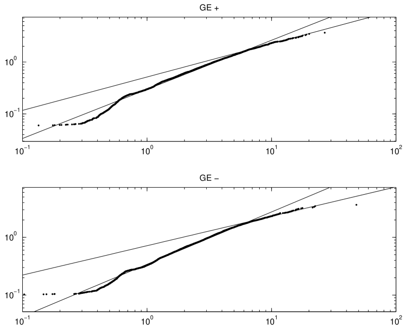
Figure 15: Graph of Gaussianized General Electric returns versus General Electric returns, for the time interval from Jan. 1970 to Dec. 2000. The upper graph gives the positive tail and the lower one the negative tail. The two straight lines represent the curves $y=\sqrt{2}\left(\frac{x}{\langle\chi_{\pm}\rangle}\right)^{\langle c_{\pm}\rangle}$ and $y=\sqrt{2}\left(\frac{x}{\chi_{\pm}}\right)^{c_{\pm}}$

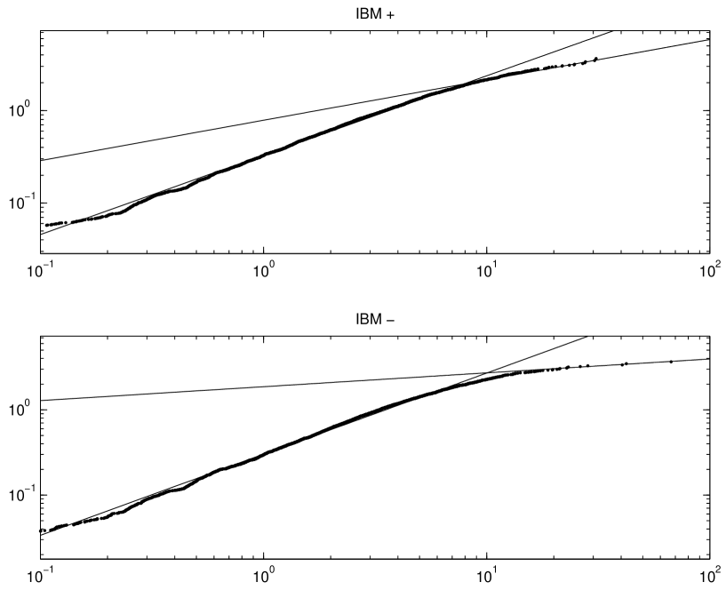
Figure 16: Graph of Gaussianized IBM returns versus IBM returns, for the time interval from Jan. 1970 to Dec. 2000. The upper graph gives the positive tail and the lower one the negative tail. The two straight lines represent the curves $y=\sqrt{2}\left(\frac{x}{\langle\chi_{\pm}\rangle}\right)^{\langle c_{\pm}\rangle}$ and $y=\sqrt{2}\left(\frac{x}{\chi_{\pm}}\right)^{c_{\pm}}$

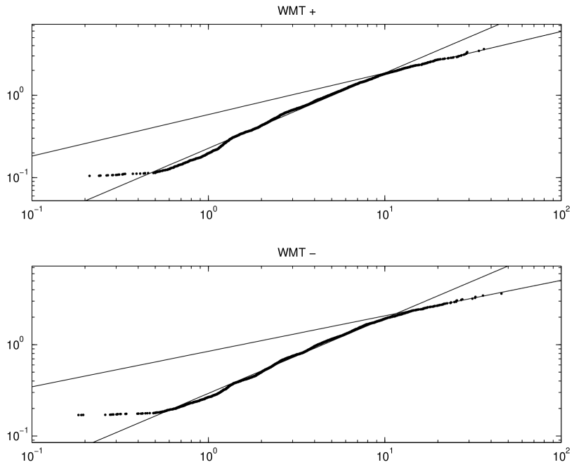
Figure 17: Graph of Gaussianized Wall Mart returns versus Wall Mart returns, for the time interval from Sep. 1972 to Dec. 2000. The upper graph gives the positive tail and the lower one the negative tail. The two straight lines represent the curves $y=\sqrt{2}\left(\frac{x}{\langle\chi_{\pm}\rangle}\right)^{\langle c_{\pm}\rangle}$ and $y=\sqrt{2}\left(\frac{x}{\chi_{\pm}}\right)^{c_{\pm}}$

References

- [Acerbi (2002)] Acerbi, C., 2002, Spectrale measures of risk : a coherent representation of subjective risk aversion, Journal of Banking and Finance.
- [Alexander and Baptista (2002)] Alexander, G.J. and A.M. Baptista, 2002, Economic implications of using a mean-VaR model for portfolio selection: A comparison with mean-variance analysis, Journal of Economic Dynamics and Control 26, 1159-1193.
- [Abramovitz and Stegun (1972)] Abramovitz, E. and I.A. Stegun, 1972, Handbook of Mathematical functions (Dover Publications, New York).
- [Allais (1953)] Allais, M., 1953, Le comportement de l’homme rationel devant le risque, critique des postulat de l’école américaine, Econometrica 21, 503-546.
- [Allais (1990)] Allais, M., 1990, Allais Paradox, in The new palgrave, Utility and probability, Macmillan, 3-9.
- [Andersen and Sornette (2001)] Andersen, J.V., and D. Sornette, 2001, Have your cake and eat it too: increasing returns while lowering large risks! Journal of Risk Finance 2, 70-82.
- [Artzner et al. (1997)] Artzner, P., F. Delbaen, J.M. Eber and D. Heath, 1997, Thinking coherently, Risk 10, 68-71.
- [Artzner et al. (1999)] Artzner, P., F. Delbaen, J.M. Eber and D. Heath, 1999, Coherent measures of risk, Math. Finance 9, 203-228.
- [Bouchaud et al. (1998)] Bouchaud, J.-P., D. Sornette, C. Walter and J.-P. Aguilar, 1998, Taming large events: Optimal portfolio theory for strongly fluctuating assets, International Journal of Theoretical and Applied Finance 1, 25-41.
- [Dowd (2000)] Dowd, K., 2000, Adjusting for risk: an improved Sharpe ratio, International Review of Economics and Finance 9, 209-222.
- [Embrechts et al. (1997)] Embrechts, P., C. Kluppelberg and T. Mikosh, 1997, Modelling extremal events (Springel-Verlag, Applications of Mathematics 33).
- [Embrechts et al. (1998)] Embrecht, P., A. McNeil and D. Straumann, 1998, Correlation and Dependence in risk management: properties and pitfalls, Proceedings of the Risk Management workshop at the Newton Institute Cambridge, Cambridge University Press.
- [Fang and Lai (1997)] Fang, H. and T. Lai, 1997, Co-kurtosis and capital asset pricing, Financial Review 32, 293-307.