Nonlinear Mechanical Response of DNA due to Anisotropic Bending Elasticity

Abstract

The response of a short DNA segment to bending is studied, taking into account the anisotropy in the bending rigidities caused by the double-helical structure. It is shown that the anisotropy introduces an effective nonlinear twist-bend coupling that can lead to the formation of kinks and modulations in the curvature and/or in the twist, depending on the values of the elastic constants and the imposed deflection angle. The typical wavelength for the modulations, or the distance between the neighboring kinks is found to be set by half of the DNA pitch.

Pacs numbers: 87.15.-v, 36.20.-r, 61.41.+e

Genetic information in living cells is carried in the linear sequence of nucleotides in DNA. Each molecule of DNA contains two complementary strands of nucleotides that are matched by the hydrogen bonds of the G-C and A-T base pairs (bps). The DNA double-helix can be found in several forms that differ from each in the geometrical characteristics such as diameter and handedness. Under normal physiological conditions DNA adopts the B-form, in which it consists of two helically twisted sugar-phosphate backbones with a diameter $2.4$ nm, which are stuffed with base pairs. The helix is right-handed with $10$ bps per turn, and the pitch of the helix is $3.4$ nm. While understanding some aspects of DNA functioning requires the details of the chemical bindings etc., there are quite a number of processes in cell that involve major structural and conformational changes in DNA, where typically a small segment of DNA interacts with certain proteins [1].

For example, consider the transcription reaction catalyzed by RNA polymerase, which creates an RNA strand that is complementary to the transcribed DNA strand. The catalysis takes place inside the transcription bubble: this is an $18$ bp stretch of unwound DNA helix stabilized by RNA polymerase, which harbors a $12$ bp RNA-DNA hybrid [2]. Low resolution structure of E. coli RNA polymerase has shown a thumb-like projection that seemingly closes around the DNA, and bends it to about $90^{\circ}$-$120^{\circ}$ [3]. There are also similar visualizations of DNA polymerase, suggesting that the enzyme bends a piece of DNA inside it [4]. In nucleosomes, a $150$ bp long segment of DNA wraps about $1.6$ turns around the histone complex that has a diameter of about $11$ nm [5]. In all of these DNA-protein complexes, a DNA fragment is subjected to a bending of the order of about $4^{\circ}$-$7^{\circ}$ per base pair, which is typically a large curvature.

The idea of studying the response of DNA to mechanical stresses is as old as the discovery of the double-helix structure itself [6]. An elastic description of DNA has been developed over the past 20 years, taking on different approaches that include Lagrangian mechanics [7, 8], statistical mechanics [9], and molecular dynamics simulation [10]. Motivated by the aforementioned structures in various DNA-protein complexes, we study the bending of short DNA segments using an elastic model. We assume that the length-scale set by the helix pitch $P\simeq 3.4\;{\rm nm}$ that involves $10$ base pairs, is long enough so that we can use a continuum elastic theory, and yet short enough that the spatial anisotropy due to the double-helical structure of DNA matters. The elastic model of DNA is used with anisotropic bending rigidities, while neglecting the linear phenomenological twist-bend [11] and twist-stretch [12] couplings. Whereas an isotropic elastic model predicts uniform bending and twisting, we find that the anisotropy in the bending rigidity introduces an effective nonlinear twist-bend coupling [13, 14] that could lead to a variety of bending and twisting structures.

Depending on the relative strengths of the elastic constants and the overall amount of deflection, we observe six different regimes: (1) A regime in which curvature is localized in the form of kinks in a periodic arrangement accompanied by simultaneous suppression of twist, while the kinks are separated by virtually flat (rod-like) and uniformly twisted segments, (2) a regime with synchronized smooth modulations of the curvature and the twist, where a rise in curvature corresponds to suppression of twist and vice versa, (3) a regime with uniform curvature and modulated twist, (4) a regime with the kink-rod structure in the curvature and uniform twist, (5) a regime with modulated curvature and uniform twist, and (6) a regime with both uniform curvature and uniform twist. These different “forms” of bent DNA are presented in Fig. 1 below, and in Fig. 2 it is specified for what values of the parameters each form appears. We find that the period of modulations as well as the distance between neighboring kinks is always set by half of the DNA pitch, i.e. 5 bps, to a good approximation. For a general DNA segment bending is always found to reduce the linking number due to the effective (nonlinear) twist-bend coupling. When the length of the DNA segment is equal to an integer multiple of 5 bps, however, we observe a transition from an over-twisted regime where there are kinks located exactly at the end points to an under-twisted regime where the kinks are located exclusively in the interior. The boundary corresponding to this transition in the parameter space of the elastic constants is plotted in Fig. 3.

The elastic model of DNA represents the molecule as a slender cylindrical elastic rod. The rod is parametrized by the arclength $s$, and at each point, an orthonormal basis is defined with $\hat{e}_{1}$, $\hat{e}_{2}$, and $\hat{e}_{3}$, corresponding to the principal axes of the elastic rod. In the undeformed state, all the systems are parallel, with the $\hat{e}_{3}$-axes being all parallel to the axis of the rod. The deformation of the elastic rod is then parametrized by a mapping that relates the local coordinate system to a reference one, specified by the Euler angles $\theta(s)$, $\phi(s)$, and $\psi(s)$. The elastic energy is written as [15]

$$\beta E=\frac{1}{2}\int_{0}^{L}ds\;[A_{1}\Omega_{1}^{2}+A_{2}\Omega_{2}^{2}+C(\Omega_{3}-\omega_{0})^{2}],$$ (1)

in the dimensionless units, where $A_{1}$ and $A_{2}$ are the bending rigidities, $C$ is the twist rigidity, and $\omega_{0}=2\pi/P=1.85\;{\rm nm}^{-1}$ is the spontaneous twist of the helix. In terms of Euler angles, we have $\Omega_{1}(s)=(d\theta/ds)\sin\psi-(d\phi/ds)\sin\theta\cos\psi$, $\Omega_{2}(s)=(d\theta/ds)\cos\psi+(d\phi/ds)\sin\theta\sin\psi$, and $\Omega_{3}(s)=(d\psi/ds)+(d\phi/ds)\cos\theta$. Without loss of generality, we assume that the rod will stay planar even after the application of a bending force, and hence set $d\phi/ds=0$. The bending is characterized by an overall angle $\theta_{0}$, and we assume that the bent segment of DNA is attached to undeformed tails, so that it corresponds to bending of a piece of a long DNA. Since the tails have a uniform twist characterized by $\omega_{0}$, we assume that the twist at the two ends of the DNA segment is also $\omega_{0}$, to preserve continuity.

After defining $A\equiv\frac{1}{2}(A_{1}+A_{2})$, $A^{\prime}\equiv\frac{1}{2}(A_{2}-A_{1})$, and setting $s=Lt$, we have

$$\beta E=\frac{A^{\prime}\theta_{0}^{2}}{2L}\int_{0}^{1}dt \left[\left(\frac{A}{A^{\prime}}+\cos 2\psi\right)\frac{\dot{\theta}^{2}}{\theta_{0}^{2}}\right.$$ (3)

$$\left.+\frac{C}{A^{\prime}\theta_{0}^{2}}\left(\dot{\psi}-\omega_{0}L\right)^{2}\right],$$

where we have used $\dot{\theta}\equiv\frac{d\theta}{dt}$ and $\dot{\psi}\equiv\frac{d\psi}{dt}$. The above equation shows manifestly that there are three effective dimensionless parameters in the system: $A/A^{\prime}$, $C/(A^{\prime}\theta_{0}^{2})$, and $\omega_{0}L$. We can find the extremum of $\beta E$ by applying standard variational techniques to Eq. (3). The resulting Euler-Lagrange equations for $\theta(t)$ and $\psi(t)$ are found as

$$\frac{\ddot{\theta}}{\theta_{0}}=\frac{2\dot{\psi}(\dot{\theta}/\theta_{0})\sin 2\psi}{\left(\frac{A}{A^{\prime}}+\cos 2\psi\right)},$$ (4)

and

$$\ddot{\psi}=-\left(\frac{C}{A^{\prime}\theta_{0}^{2}}\right)^{-1}\left(\frac{{\dot{\theta}}^{2}}{\theta_{0}^{2}}\right)\sin 2\psi.$$ (5)

The above equations should be solved subject to the boundary conditions $\dot{\psi}(0)=\dot{\psi}(1)=\omega_{0}L$, $\theta(0)=0$ and $\theta(1)=\theta_{0}$. While the mean bending rigidity $A$ is known to be about $50$ nm in the salt-saturation limit [9], and the twist rigidity $C$ is believed to be roughly $75$ nm [16], little is known about the parameter $A^{\prime}$ that describes the anisotropy. Hence, we solve the above set of coupled nonlinear equations numerically for various values of the parameters $A/A^{\prime}$ and $C/(A^{\prime}\theta_{0}^{2})$, and for several DNA lengths.

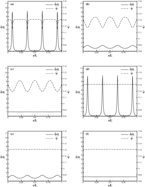
FIG. 1.: Different possible conformations of the DNA for various values of $C/(A^{\prime}\theta_{0}^{2})$ and $A/A^{\prime}$. The DNA length is $18$ bps. The solid lines show the normalized curvature $\dot{\theta}/\theta_{0}$ and the dotted lines show the twist $\dot{\psi}$. (a) Kink-rod curvature structure and a corresponding singular suppression of twist at the kinks. The plot corresponds to $A/A^{\prime}=1.02$ and $C/(A^{\prime}\theta_{0}^{2})=0.5$. (b) Modulated curvature and twist. The plot corresponds to $A/A^{\prime}=3$ and $C/(A^{\prime}\theta_{0}^{2})=0.5$. (c) Uniform curvature and modulated twist. The plot corresponds to $A/A^{\prime}=79$ and $C/(A^{\prime}\theta_{0}^{2})=0.5$. (d) Kink-rod curvature structure and uniform twist. The plot corresponds to $A/A^{\prime}=1.02$ and $C/(A^{\prime}\theta_{0}^{2})=30$. (e) Modulated curvature and uniform twist. The plot corresponds to $A/A^{\prime}=3$ and $C/(A^{\prime}\theta_{0}^{2})=30$. (f) Uniform curvature and uniform twist. The plot corresponds to $A/A^{\prime}=79$ and $C/(A^{\prime}\theta_{0}^{2})=30$.

We observe that the above equations can acquire more than one solution depending on the values of the parameters, with the different DNA conformations characterized by deferent energies and different values of the linking number, defined as $Lk=[\psi(1)-\psi(0)]/(2\pi)$ [17]. Note that for an undeformed DNA we have $Lk_{0}=\omega_{0}L/(2\pi)$. For each value of DNA length that is not an integer multiple of 5 bps, we find six distinct types of behaviors for various values of $A/A^{\prime}$ and $C/(A^{\prime}\theta_{0}^{2})$, as presented in Fig. 1 and described above. For all of these conformations, which correspond to the lowest energy case among the different possible solutions, the change in the linking number $\Delta Lk=Lk-Lk_{0}$ is negative, and DNA is thus under-twisted.

We also observe in all of these cases that the periodicity of the curves, whether there are modulations or kinks, is set by half of the DNA pitch, i.e. $5$ bps, to a good approximation. This can be understood by looking at the first-integrals of Eqs. (4) and (5), which can be calculated as

$$\frac{\dot{\theta}}{\theta_{0}}=\frac{\alpha_{1}}{\left(\frac{A}{A^{\prime}}+\cos 2\psi\right)},$$ (6)

and

$$\dot{\psi}^{2}=-\frac{\alpha_{1}^{2}}{\left(\frac{C}{A^{\prime}\theta_{0}^{2}}\right)\left(\frac{A}{A^{\prime}}+\cos 2\psi\right)}+\alpha_{2},$$ (7)

respectively, where $\alpha_{1}$ and $\alpha_{2}$ are the integration constants. Using a linear approximation $\psi\approx 2\pi s/P$, we can then expect a periodic behavior for both ${\dot{\theta}}$ and ${\dot{\psi}}$ in Eqs. (6) and (7), with a period of $P/2$.

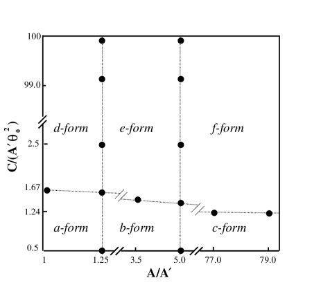
FIG. 2.: A diagram delineating the different regimes corresponding to the six distinct forms of bent DNA, depending on the values of $C/(A^{\prime}\theta_{0}^{2})$ and $A/A^{\prime}$. The DNA length is $18$ bps. For fixed values of the elastic constants $A$, $A^{\prime}$, and $C$, bending of DNA at various angles would correspond to vertical lines. Note that in this case, the only permissible transitions are from d-form to a-form, from e-form to b-form, and from f-form to c-form, because the zone boundaries are also vertical.

When the ratio $A/A^{\prime}$ (that is by definition always greater than 1) is somewhat close to 1, the combination $A/A^{\prime}+\cos 2\psi$ could be close to zero, and then Eq. (6) implies that $\dot{\theta}/\theta_{0}$ must be large. This corresponds to the kinks in the curvature. In this case, for sufficiently small $C/(A^{\prime}\theta_{0}^{2})$ (numerically we find $<1.6$), Eq. (7) implies that the same effect should simultaneously happen in the twist, which corresponds to Fig. 1a. For larger $C/(A^{\prime}\theta_{0}^{2})$, however, this pattern should disappear from the twist structure leaving only a uniform twist, which corresponds to Fig. 1d.

For intermediate values of $A/A^{\prime}$, the periodicity imposed by the term $A/A^{\prime}+\cos 2\psi$ is still felt in the curvature, in the form of modulations. Again, in this case, a small value for $C/(A^{\prime}\theta_{0}^{2})$ leads to accompanying modulations in the twist, corresponding to Fig. 1b, while large $C/(A^{\prime}\theta_{0}^{2})$ will wash it out to uniform twist, corresponding to Fig. 1e. Note that an increase in the curvature always coincides with a decrease in the twist, and vice versa, as can be manifestly understood from Eqs. (6) and (7).

When $A/A^{\prime}$ is very large, the dominant term in the denominator of Eq. (6) is $A/A^{\prime}$, and hence the curvature approaches a constant value. Since the parameters are normalized such that a constant curvature should be equal to 1, we find that in this limit $\alpha_{1}\simeq A/A^{\prime}$. Then a small value of $C/(A^{\prime}\theta_{0}^{2})$ can make it possible for the modulations to be felt in the twist, corresponding to Fig. 1c, whereas for large values of $C/(A^{\prime}\theta_{0}^{2})$ these modulations are also washed out and we have a uniform twist, which corresponds to Fig. 1f.

In Fig. 2, we have summarized the above results in a diagram that delineates the different regimes corresponding to the different forms of bent DNA defined in Fig. 1, for various values of $C/(A^{\prime}\theta_{0}^{2})$ and $A/A^{\prime}$. Note that while the horizontal line (the boundary that separates a, b, and c regions from d, e, and f regions) is slightly tilted, the other two lines are virtually vertical within our numerical precision. Since for fixed values of the elastic constants $A$, $A^{\prime}$, and $C$, bending of DNA at various angles would correspond to vertical lines, the fact that the two zone boundaries are vertical requires that the only permissible transitions upon bending are from d-form to a-form, from e-form to b-form, and from f-form to c-form. This could provide an interesting possible experimental check of the present analysis.

In the a-form regime, when the DNA length is between $5n$ bps and $5(n+1)$ bps with $n$ being an integer number, the number of kinks is $n+1$. One could then ask what happens if the DNA length is exactly equal to $5n$ bps. In this case, two different sets of solutions are observed, as shown in the insets of Fig. 3: (1) A set of solutions in which there are $n$ kinks situated exclusively in the interior, leaving an almost vanishing curvature at the end-points. The value for $\Delta Lk$ in this case is negative, which means that DNA is under-twisted. (2) Another set of solutions in which there are $n-1$ kinks in the interior, and the other kink is splitted in half and located exactly at the end-points, leading to a large curvature at the two ends. In this case, $\Delta Lk$ is positive, i.e. DNA is over-twisted. We found that both of these sets of solutions could correspond to the minimum energy case, depending on the values of the parameters. The transition line between the two regimes is plotted in Fig. 3, for a DNA segment of $15$ bps.

In the present treatment thermal fluctuations have been neglected. This is justified by noting that the typical lengths considered here are much smaller than the persistence length of DNA, which is about $150$ bps, and therefore we do not expect considerable deformation fluctuations of the DNA. However, due to the presence of multiple energy minima that are not too different from each other, we do expect that the conformation of DNA jumps between the different possible minimum energy solutions, provided that the barrier is not too large. This could be particularly interesting if the bent DNA is involved in a dynamical process, such as transcription [18].

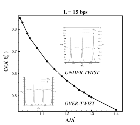
FIG. 3.: A diagram showing the different conformations of DNA, when its length is an integer multiple of 5 bps. A transition is observed from an over-twisted regime where there are kinks located exactly at the end-points, to an under-twisted regime where the kinks are located exclusively in the interior.

In conclusion, we have studied the response of a finite DNA segment to bending, taking into account the anisotropy in the bending rigidity caused by the double-helical structure. We have shown that the nonlinear twist-bend coupling caused by the anisotropy can lead to formation of kink-rod patterns and modulations in the curvature and/or twist. This effect may be related to the recent observation in high resolution X-ray, that DNA is not uniformly bent around the histone octamer and its curvature is larger at some places in the nucleosome [5]. We finally note that the present analysis can be also applied to other biopolymers—the best candidate for an experimental realization of these effects will probably be F-actin, which has a much longer persistence length and can thus be more easily manipulated in its stiff limit.

We are grateful to M.A. Jalali and T.B. Liverpool for helpful discussions and comments.

REFERENCES

- [1] B. Alberts, J. Lewis, M. Raff, K. Roberts, and J.D. Watson, Molecular Biology of the Cell, (Garland, New York, 1994).
- [2] L. Stryer, Biochemistry, 4th edition (Freeman, 1995).
- [3] S.A. Darst, E.W. Kubalek, and R.D. Kornberg, Nature 340, 730 (1989); A. Polyakov, E. Severinov, and S.A. Darst, Cell 83, 365 (1995).
- [4] L.S. Beese, V. Derbyshire, and T.A. Steitz, Science 260, 352 (1993); J.R. Kiefer, C. Mao, J.C. Braman, and L.S. Beese, Nature 391, 304 (1998).
- [5] K. Luger, A.W. Mäder, R.K. Richmond, D.F. Sargent, and T. Richmond, Nature 389, 251 (1997).
- [6] M.H.F. Wilkins, R.G. Gosling, and W.E. Seeds, Nature 167, 759 (1951).
- [7] C.J. Benham, Biopolymers 22, 2477 (1983); M. Le Bret, Biopolymers 23, 1835 (1984); F. Tanaka and H. Takahash, J. Chem. Phys. 83, 6017 (1985); H. Tsuru, and M. Wadati, Biopolymers 25, 2083 (1986).
- [8] B. Fain, J. Rudnick, and S. Östlund, Phys. Rev. E 55, 7364 (1997); B. Fain and J. Rudnick , Phys. Rev. E 60, 7239 (1999); R. Zandi and J. Rudnick Phys. Rev. E 64, 051918 (2001).
- [9] J.F. Marko and E.D. Siggia, Phys. Rev. E 52, 2912 (1995).
- [10] T. Schlick and W. Olsen, Science 257, 1110 (1992).
- [11] J.F. Marko and E.D. Siggia, Macromolecules 27, 981 (1994); 29, 4820(E) (1996).
- [12] R.D. Kamien, T.C. Lubensky, P. Nelson, and C.S. O’Hern, Europhys. Lett. 38, 237 (1997).
- [13] T.B. Liverpool, R. Golestanian, and K. Kremer, Phys. Rev. Lett. 80, 405 (1998); R. Golestanian and T.B. Liverpool, Phys. Rev. E 62, 5488 (2000).
- [14] A. de Col and T.B. Liverpool, preprint cond-mat/0203561.
- [15] L. Landau and E. Lifshitz, Theory of elasticity, 3rd edition (Pergamon, 1986).
- [16] A.V. Vologodskii, S.D. Levene, K.V. Klenin, M. Frank-Kamenetskii, and N.R. Cozzarelli, J. Mol. Biol. 272, 1224 (1992).
- [17] Linking Number is a topological invariant for linear objects such as the elastic rod, and according to White’s theorem it can be written as the sum of two terms: the twist and the writhe. In the general case, we can write a simple expression for linking number using the Euler-angle description as [8], which simplifies to in our case because .
- [18] F. Mohammad-Rafiee and Ramin Golestanian, work in progress.