On solutions of a class of non-Markovian Fokker-Planck equations

Abstract

We show that a formal solution of a rather general non-Markovian Fokker-Planck equation can be represented in a form of an integral decomposition and thus can be expressed through the solution of the Markovian equation with the same Fokker-Planck operator. This allows us to classify memory kernels into safe ones, for which the solution is always a probability density, and dangerous ones, when this is not guaranteed. The first situation describes random processes subordinated to a Wiener process, while the second one typically corresponds to random processes showing a strong ballistic component. In this case the non-Markovian Fokker-Planck equation is only valid in a restricted range of parameters, initial and boundary conditions.

Many physical phenomena related to relaxation in complex systems are described by non-Markovian Fokker-Planck equations in a form

$$\frac{\partial}{\partial t}P({\bf x},t)=\int K(t-t^{\prime}){\cal L}P({\bf x},t^{\prime})dt^{\prime},$$ (1)

where $K(t)$ is a memory kernel and where ${\cal L}$ is a linear operator acting on variable(s) ${\bf x}$. Such equations are often postulated on the basis of linear-response considerations for different physical situations and in several cases can be more or less rigorously derived based on a microscopic description. In the symmetric case, the usual form of the operator ${\cal L}$ reads:

$${\cal L}P({\bf x},t)=D\left(-\nabla\frac{{\bf f}({\bf x})}{k_{B}T}P({\bf x},t)+\Delta P({\bf x},t)\right),$$ (2)

where $D$ is the diffusion coefficient (here supposed to be coordinate-independent) and ${\bf f}(x)=-\nabla U({\bf x})$ is a potential force. Depending on boundary conditions, the operator Eq.(2) may or may not possess an equilibrium state $P({\bf x},t)=W({\bf x})$, which corresponds to the solution of the equation $-(k_{B}T)^{-1}{\bf f}({\bf x})W({\bf x})+\nabla W({\bf x})=0$, so that $W({\bf x})=\exp(-U({\bf x})/k_{B}T)$ is a Boltzmann distribution. In this case Eq.(2) can be rewritten in the form

$${\cal L}P({\bf x},t)=D\sum_{\alpha,\beta}\frac{\partial}{\partial x_{\alpha}}W({\bf x)}\frac{\partial}{\partial x_{\beta}}\frac{P({\bf x},t)}{W({\bf x)}},$$ (3)

which is known to appear naturally when describing thermodynamics of complex systems when reducing their behavior to a few relevant variables (thermodynamical observables $x_{\alpha}$) as is done e.g. in the Zwanzig’s approach Zwanz1 . Compared to the general form of Ref. Zwanz1 , Eq.(1) lacks the drift term; in some cases this general form can be reduced to Eq.(1), say by a Galilean transformation, see MKS ; MeK2 .

The Eq.(1) with a $\delta$-functional memory kernel $K(t)=\delta(t)$ corresponds to a usual Fokker-Planck equation (FPE) describing Markovian processes. The solution of this equation is known to be a proper probability density (so that $P({\bf x},t)\geq 0$ and $\int P({\bf x},t)d{\bf x}=1$) if the stationary state exists (i.e. whenever the Fokker-Planck operator possesses a zero eigenvalue), otherwise it is a non-proper probability density ($P({\bf x},t)\geq 0$ and $\int P({\bf x},t)d{\bf x}\leq 1$).

Many special forms of memory kernels are of interest. We note that fractional Fokker-Planck equations widely discussed as a relevant mathematical tool for the description of many complex phenomena MeK2 belong just to the class described by Eq.(3) with $K(t)$ being a power function of $t$: $K(t)\propto t^{-\alpha}$, and that the so-called distributed-order fractional equations, introduced on the phenomenological basis in Ref. Caputo and describing slow processes lacking scaling Chech correspond to related kernels in a form $K(t)\propto\int f(\alpha)t^{-\alpha}d\alpha$. On the other hand, much less exotic exponential kernels, describing the rather fast memory decay, are ubiquitous. More complex kernels are encountered when describing reactions in polymer systems Cherayil ; Ghosh .

The subdiffusive processes described by fractional Fokker-Planck equations with $1<\alpha<2$ are known to be subordinated to a Wiener process Sok1 ; Barkai , so that the solution of this equation can be obtained through an integral transformation of the solution of a usual (Markovian) FPEs with the same potential, initial and boundary conditions. As we proceed to show, some analogue statements can be done also for the general version of the non-Markovian FPE. The properties of such a transform and some important consequences of its existence will be discussed in what follows.

Let us show that the formal solution of the non-Markovian Fokker-Planck equation can be obtained in a form of an integral decomposition

$$P({\bf x},t)=\int_{0}^{\infty}F({\bf x},\tau)T(\tau,t)d\tau,$$ (4)

where $F({\bf x},\tau)$ is a solution of a Markovian FPE with the same Fokker-Planck operator ${\cal L}$

$$\frac{\partial}{\partial t}F({\bf x},t)={\cal L}F({\bf x},t),$$ (5)

and for the same initial and boundary conditions, and the function $T(\tau,t)$ is connected with the memory kernel $K(t)$ Sok1 ; Barkai . Parallel to Ref. Sok1 we shall call $\tau$ the internal variable of decomposition, and ${\bf x}$ and $t$ its external variables. Moreover, we show that the Laplace-transform $\tilde{T}(\tau,u)$ of $T(\tau,t)$ in its external variable, $\tilde{T}(\tau,u)=\int_{0}^{\infty}T(\tau,t)e^{-ut}dt$ reads:

$$\tilde{T}(\tau,u)=\frac{1}{\tilde{K}(u)}\exp\left[-\tau\frac{u}{\tilde{K}(u)}\right],$$ (6)

where $\tilde{K}(u)$ is a Laplace-transform of the memory kernel $K(t)$. Eq.(6) means that the Laplace-transform of $P({\bf x},t)$ in its temporal variable reads:

$$\tilde{P}({\bf x},u) = \int_{0}^{\infty}dte^{-ut}\int_{0}^{\infty}d\tau F({\bf x},\tau)T(\tau,t)$$ (7)

$$= \int_{0}^{\infty}d\tau F({\bf x},\tau)\tilde{T}(\tau,u)$$

$$= \int_{0}^{\infty}d\tau F({\bf x},\tau)\frac{1}{\tilde{K}(u)}\exp\left[-\tau\frac{u}{\tilde{K}(u)}\right]$$

$$= \frac{1}{\tilde{K}(u)}\tilde{F}\left({\bf x},\frac{u}{\tilde{K}(u)}\right),$$

where $\tilde{F}({\bf x},u)$ is a Laplace-transform of $F({\bf x},\tau)$ in its second variable $\tau$. Let us now note that the Laplace-transform of the non-Markovian FPE, Eq.(1) reads:

$$u\tilde{P}({\bf x},u)-P(x,0)=K(u){\cal L}\tilde{P}({\bf x},u),$$ (8)

where $P(x,0)$ is the initial condition. Inserting the form, Eq.(7), into Eq.(8) one gets:

$$\frac{u}{K(u)}\tilde{F}\left({\bf x},\frac{u}{K(u)}\right)-P({\bf x},0)={\cal L}\tilde{F}\left({\bf x},\frac{u}{K(u)}\right).$$ (9)

Introducing a new variable $s=u/K(u)$ we rewrite Eq.(9) in a form

$$s\tilde{F}\left({\bf x},s\right)-P({\bf x},0)={\cal L}\tilde{F}\left({\bf x},s\right),$$ (10)

in which one readily recognizes the Laplace-transform of an ordinary, Markovian FPE, Eq.(5), with the same initial condition $P({\bf x},0)$. This completes our proof. Thus, the solution of a non-Markovian Fokker-Planck equation of the type of Eq.(1) in the Laplace domain is connected with the solution of the regular Fokker-Planck equation through

$$\tilde{P}({\bf x},u)=\frac{1}{\tilde{K}(u)}\tilde{F}\left({\bf x},\frac{u}{\tilde{K}(u)}\right).$$ (11)

In the time domain this corresponds to Eq.(4), where $T(\tau,t)$ is given by Eq.(6).

The existence of the formal solution of the non-Markovian FPE in form of Eq.(11) brings several advantages: It gives an analytical tool to express the solution of the non-Markovian problem through the solution of the Markovian one, which is often known (at least for simple potentials and simple boundary conditions). Even if the solutions are not known analytically, a numerical procedure based on Eq.(4) can be much simpler than the direct solution of Eq.(1). Moreover, in many cases the non-negativity of the solution of a non-Markovian FPE (assumed to be a probability density) can be easily proved without solving the equation. This is true for a wide class of relaxation processes subordinated to a Wiener process, i.e. for the equations with ”safe” kernels (vide infra).

Note that $F({\bf x},t)$ is for each ${\bf x}$ a nonnegative function of $t,$ since it is a (possibly, non-proper) probability density function (pdf) in ${\bf x}$. A function $f(u)$ is a Laplace-transform of a nonnegative function defined on $\left[0,\infty\right)$ if and only if $f(u)$ is completely monotone, i.e. $f(0)>0$ and $(-1)^{n}f^{(n)}(u)\geq 0$, see Chap. XIII of Ref. Feller . Remember now, that $P({\bf x},u)=\tilde{F}\left({\bf x},u/\tilde{K}(u)\right)/\tilde{K}(u)$ where the function $\tilde{F}\left({\bf x},s\right)$ is completely monotone in its second variable. This allows us to classify all kernels into the ”safe” ones, for which $\tilde{P}({\bf x},u)$ is completely monotone for any completely monotone function $\tilde{F}\left({\bf x},u\right)$, and the ”dangerous” ones, when this is not the case. Noting that the product of two completely monotone functions is a completely monotone function and that a function of the type $f(g(u))$ is completely monotone, if $f(s)$ is completely monotone and if the function $g(u)$ is positive and possesses a completely monotone derivative Feller , we can easily formulate a sufficient condition for safety: It is the case if both functions, $\tilde{K}(u)$ and $u/\tilde{K}(u)$ are positive and possess completely monotone derivatives. As we proceed to show, in this case $T(\tau,t)$ is a pdf in its first variable. The kernels for which this is the case are ”safe” in the sense that whatever the Fokker-Planck operator ${\cal L}$ is (i.e. whatever the potential, the initial and the boundary conditions are), the solutions of the non-Markovian FPE will be nonnegative and physically sound. The dangerous kernels correspond to the situations when the physical solutions of the non-Markovian Fokker-Planck equations exist only in the restricted domain of parameters.

The function $T(\tau,t)$ is always normalized to unity with respect to variable $\tau$. To see this, let us consider $J(t)=$ $\int_{0}^{\infty}d\tau T(\tau,t)$. Its Laplace transform is $\tilde{J}(u)=\int_{0}^{\infty}d\tau\tilde{T}(\tau,u)=\tilde{K}^{-1}(u)\int_{0}^{\infty}d\tau\exp\left[-\tau u/\tilde{K}(u)\right]=1/u$, so that $\tilde{J}(t)\equiv 1$. On the other hand, $T(\tau,t)$ may or may not be a probability distribution of $\tau$ on $\left[0,\infty\right)$, depending on whether this function is non-negative or may take negative values. For all safe kernels $T(\tau,t)$ is a probability distribution: $\tilde{T}(\tau,u)$ has just the form $\tilde{T}(\tau,u)=\exp\left[-\tau u/\tilde{K}(u)\right]/\tilde{K}(u)$, i.e. corresponds exactly to the form mentioned above where we take $\exp(-\tau u)$ instead of function $\tilde{F}$. The non-negativity of the solutions of the non-Markovian FPEs then immediately follows from the fact that the integrand in Eq.(4) is a product of two non-negative functions.

Let us now consider a few examples.

Example 1. As a simplest example let us consider the Markovian situation, in which $K(t)=\delta(t)$, so that $K(u)=1$. The function $\tilde{T}(\tau,u)=K(u)^{-1}\exp\left[-\tau u/K(u)\right]=$ $\exp\left[-\tau u\right]$, so that $T(\tau,t)=\delta(t-\tau)$, and the decomposition, Eq.(4), is an identity transform.

Example 2. An example of a safe kernel is a power-law kernel $K(t)\simeq t^{-\alpha}$ with $1<\alpha<2$: both its Laplace-transform is $\tilde{K}(u)=\Gamma(1-\alpha)u^{\alpha-1}$ and the function $u/\tilde{K}(u)=u^{2-\alpha}/\Gamma(1-\alpha)$ are positive and have a completely monotone derivative. Note that such power-law kernels just correspond to the fractional Fokker-Planck equations (with the additional fractional derivative of the order $\gamma=\alpha-1$ in their right-hand side, i.e. with $0<\gamma<1$), which got now to be popular tools in describing slow relaxation MeK2 . These equations are absolutely safe Sok1 ; Barkai . The same is valid for the kernels of the distributed-order equations, $K(t)\propto\int f(\alpha)t^{-\alpha}d\alpha$ as long as the function $f(\alpha)$ vanishes outside of the interval $(1,2)$, Ref. Chech .

Example 3. As an example of a dangerous kernel we consider a simple exponentially decaying one $K(t)=r\exp(-rt)$ (the form is taken to be normalized in a way that for $r\rightarrow\infty$ it tends to a $\delta$-function). The Laplace-transform of this kernel reads: $\tilde{K}(u)=r/(u+r)$, so that $u/\tilde{K}(u)=\left(u^{2}+ru\right)/r$. Here the first and the second derivative of the last function have the same positive sign; thus it is not completely monotone. Let us show, that the non-Markovian FPE with such a kernel may lead to negative solutions.

This really is the case if the system’s behavior in a constant field is considered. In what follows we restrict ourselves to a one-dimensional situation. The Green’s function solution of the FPE in a constant field (initial condition $F(x,0)=\delta(x)$) reads:

$$F(x,\tau)=\frac{1}{2\sqrt{\pi D\tau}}\exp\left[-\frac{\left(x-\mu f\tau\right)^{2}}{4D\tau}\right]$$ (12)

with $\mu=D/k_{B}T$, so that its Laplace-transform in its temporal variable is:

$$\tilde{F}(x,s) = \frac{\exp(\mu fx/2D)}{2\sqrt{\pi D}}\times$$ (13)

$$\times \int_{0}^{\infty}\frac{1}{\sqrt{t}}\exp\left[-\left(\frac{\mu^{2}f^{2}}{4D}+s\right)t-\frac{x^{2}}{4D}t^{-1}\right]dt=$$

$$= \frac{\exp(2\zeta\lambda)}{2\sqrt{D}}\frac{1}{\sqrt{\zeta^{2}+s}}\exp\left[-2\sqrt{(\zeta^{2}+s)\lambda^{2}}\right]$$

(see 2.3.16.2 of Ref.BP ), where the variables $\lambda=x/2\sqrt{D}$ and $\zeta=\mu f/2\sqrt{D}$ are introduced. The function $\tilde{P}(x,u)$ is obtained from $\tilde{F}(x,s)$ by multiplying by $1/\tilde{K}(u)$ and by substitution $s=u/\tilde{K}(u)$, so that

$$\tilde{P}(x,u) = \frac{\exp(2\zeta\lambda)}{2\sqrt{D}}\frac{(u+r)/r}{\sqrt{\zeta^{2}+u(u+r)/r}}\times$$ (14)

$$\times \exp\left[-2\left|\lambda\right|\sqrt{\zeta^{2}+u(u+r)/r}\right]$$

This function is not completely monotone: Its first derivative (which has to be always negative in the case of a pdf) changes sign, getting (for small $u$, i.e. in the long-time asymptotic) positive for $\zeta>(2r)^{-1}\left(\left|\lambda\right|r^{2}+\sqrt{\lambda^{2}r^{4}+2r^{3}}\right)$ (here we took $\zeta>0$, so that the overall distribution moves to the right). The oscillations occur initially at small $\left|\lambda\right|$, corresponding to the initial position. Since the maximum of the pdf moves to the right, they occur at the left flank of the distribution, and for $\zeta>\zeta_{c}=\sqrt{r/2}$. Thus, if the force $f$ is strong enough, $f>\sqrt{2rD}/\mu$, the solution of non-Markovian FPE ceases at long times to be a probability density, except for the Markovian case $r\rightarrow\infty$. On the other hand, for the force-free case of pure diffusion ($\zeta=0$) we have

$$\tilde{P}(x,u)=\frac{1}{2\sqrt{D}}\frac{\sqrt{(u+r)/r}}{\sqrt{u}}\exp\left[-2\left|\lambda\right|\sqrt{u\left(u+r\right)/r}\right],$$ (15)

which is a completely monotone function defining a pdf. For $u$ small ($t$ large) this function tends to a form corresponding to a Gaussian:

$$\tilde{P}(x,u)\simeq\frac{1}{2\sqrt{D}}\frac{1}{\sqrt{u}}\exp\left[-2\left|\lambda\right|\sqrt{u}\right],$$ (16)

which is our Eq.(12) with $f=0$, while for large $u$ (small $t$) we have

$$\tilde{P}(x,u\rightarrow 0)=\frac{1}{2\sqrt{Dr}}\exp\left[-2\left|\lambda\right|u/\sqrt{r}\right]$$ (17)

corresponding to

$$P(x,t)\simeq\frac{1}{2\sqrt{Dr}}\delta\left(\frac{2\left|\lambda\right|}{\sqrt{r}}-t\right)=\frac{1}{2}\delta(\left|x\right|-\sqrt{Dr}t).$$ (18)

At early times an initial pulse propagates as a wave, while at later times the propagation gets diffusive, Ref. KMS . Note that $Dr$ has a dimension of velocity squared (so that $D=v^{2}/r$ where $v$ is the typical velocity and $\tau_{c}=1/r$ is the correlation time). Thus, at short times $P(x,t)=\frac{1}{2}\delta(\left|x\right|-vt)$, and the overall equation describes the transition from a ballistic to a diffusive propagation, i.e. a kind of a Drude model. The mean-free path in the model is exactly $v\tau_{c}=\sqrt{D/r}$. The breakdown of the physical solution for larger forces gets now a clear physical meaning: The case $f>\sqrt{2rD}/\mu$ corresponds to the situation when the mean velocity gain on the mean free path is larger than the rms velocity $v=\sqrt{Dr}$, clearly the case in which the diffusion coefficient $D$ can no more be considered as force-independent (which is only possible for $\mu f\ll v$ where the force enters as a perturbation).

Thus, our analysis shows that the transition to non-positive solutions denotes leaving the region of physical validity of the model: the fact that the kernel is ”dangerous” shows, that corresponding equations are only reasonable in a restricted domain of parameters, initial and boundary conditions, and that other conditions are unphysical.

The behavior of $P(x,t)$ for the exponential kernel and for $f=0$ is shown in Fig.1, where the results of numerical inversion of Eq.(14) are shown for $t=0.5$, 1, 2 and 3. Here only the part for $x>0$ is shown since $P(x,t)$ is an even function of $x$. The overall form of the distribution with the two side peaks is typical for systems showing random-walk behavior with strong ballistic component, like Lévy walks. At difference with the Lévy-walk situation, the overall weight of the peaks decays very fast. Thus, for $t=0.5$ they absorb more than one-half of the overall probability, while for $t=3$ the most of the probability lies in the central part of the distribution, whose form slowly tends to a Gaussian.

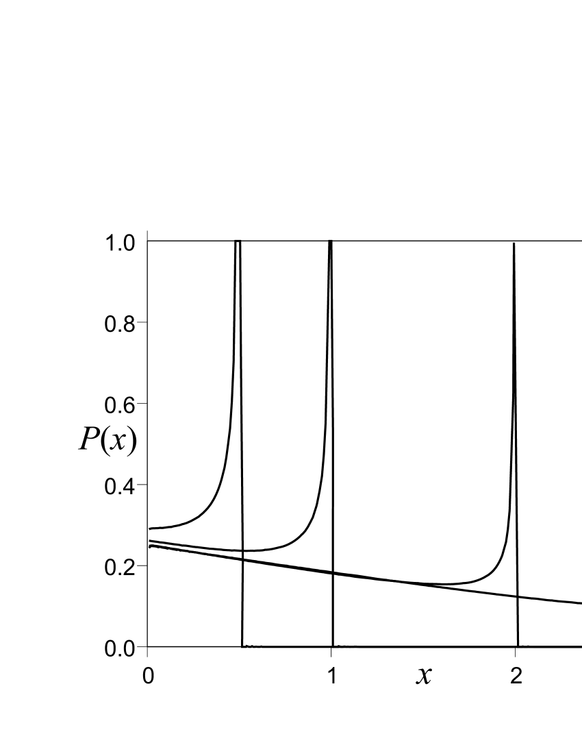
Figure 1: The time evolution of the Green’s function solution of a non-Markovian diffusion equation ($f=0$), see text for details. The parameters are $D=$ $r=1$, so that the peaks move with the velocity $v=1$. The curves correspond to $t=0.5$, 1, 2 and 3 (from left to right).

Note that the situation when the short-time behavior is ballistic and corresponds to the distribution with pronounced side peaks (stemming essentially from the solution of the Liouville equation) is typical (as a short-time behavior) for all kernels $K(t)\,$which tend to a constant value at $t\rightarrow 0$: For all of them $\tilde{K}(u)\simeq K(0)/u$ for $u$ large, so that Eq.(17) asymptotically holds. Turning to kernels behaving at short times as a power-law, $K(t)\simeq t^{-\alpha}$ (corresponding to $K(u)\simeq\Gamma(1-\alpha)u^{\alpha-1}$), we note that the kernels with $0<\alpha<1$ lead to the similar kind of behavior (bimodal pdf), see Ref. MeK1 , where the peaks are the less pronounced the larger is $\alpha$. On the other hand, safe power-law kernels with $1<\alpha<2$ lead to pdf’s showing a single peak at zero. It is also interesting to discuss the two other situations: The kernels starting from zero and the strongly decaying power-laws. Now, a situation of a kernel starting at zero, i.e. as $K(t)\simeq t^{\beta}$ with $\beta>0$, corresponds to $\tilde{K}(u)\simeq u^{-1-\beta}$ and therefore to

$$\tilde{P}(x,u)=\frac{u^{\beta/2}}{2\sqrt{D}}\exp\left[-2\left|\lambda\right|u^{1+\beta/2}\right]$$

which is not a completely monotone function (its first derivative changes sign at $u=\left[2\left|\lambda\right|(2+\beta)/\beta\right]^{-2/(2+\beta)}$), and thus is not a Laplace-transform of a pdf. The same is the case for the kernels with stronger divergence, $K(t)\simeq t^{-\alpha}$ with $\alpha>2$. Here

$$\tilde{P}(x,u)=\frac{u^{-\alpha/2}}{2\sqrt{D}}\exp\left[-2\left|\lambda\right|u^{1-\alpha/2}\right]$$

is again not a completely monotone function: its second derivative $\tilde{P}_{uu}(x,u)$ (which is essentially a quadratic form in $\left|\lambda\right|$) possesses a positive root for all $\alpha>2$. Thus, the set of kernels which correspond to physical behavior (in a force-free case) consists of kernels which behave at small $t$ as $K(t)\simeq t^{-\alpha}$ with $0\leq\alpha\leq 2$. All other kernels can be considered as approximations which are not valid at short times.

Let us make some notes about the long-time asymptotic behavior. For $t$ large all integrable kernels correspond to the behavior $K(u)\rightarrow I$ with $I=\int_{0}^{\infty}K(t)dt$, and thus lead to

$$\tilde{P}(x,u)=\frac{1}{2\sqrt{D}}\frac{1}{\sqrt{Iu}}\exp\left[-2\left|\lambda\right|\sqrt{u/I}\right]$$

i.e. to the Gaussian behavior. All these kernels correspond essentially to the processes which can at longer times be approximated by a Markovian process. The kernels whose integral diverges are exemplified by the safe power-law-like kernels $K(t)\propto t^{-\alpha}$ with $1\leq\alpha\leq 2$, where the divergence stems from the short-time behavior, and the dangerous power-laws ($0\leq\alpha<1$) where the integral diverges at infinity. Both of them correspond to non-decoupling memory. The situations are considered in detail in Refs. Sok1 ; MeK2 . The growing kernels are definitely unphysical.

Whenever the kernel is safe, the variable $\tau$ can be interpreted as an operational time, and $T(\tau,t)$ is a pdf of the operational time $\tau$ at physical time $t$, and our integral decomposition corresponds to a subordination. Whenever $T(\tau,t)$ can be considered as pdf resulting from a random process with nonnegative increments, we have to do with a continuous-time random walk situation (CTRW) or its continuous limit. The corresponding solutions of the non-Markovian FPEs (including the Green’s function solutions) can then be represented as the solutions of the ordinary FPE corresponding to different final operational times; these solutions are weighted with the distribution of this final operational time, which is given by the pdf $T(\tau,t)$. Thus, the ensemble of the sample paths corresponding to a random process described by the non-Markovian FPE with a safe kernel can be visualized as an ensemble of paths (random walks) of a process described by a corresponding Markovian equation, taken not at a given time $t$, but having different temporal ”lengths” (duration).

The dangerous kernels correspond to the situation when some of these paths enter with negative weight, so that the overall positiveness of the solution can not in general be guaranteed. We note that the case of the exponential kernel (for which the non-Markovian FPE can be rewritten in the form of the telegrapher’s equation) can be considered as an approximation for a CTRW with the waiting-time distribution being a difference of two exponentials KMS . However, neglecting higher terms in such an approximation leads to the fact that the exponential kernel is dangerous, and that the positiveness of the solution is not always guaranteed.

Let us now summarize our findings. We considered a formal solution of a rather general form of a non-Markovian Fokker-Planck equation and have shown that this can be represented in a form of integral decomposition. This allows us to classify the memory kernels into safe ones, for which the solution of the non-Markovian FPE is always a probability density, and dangerous ones, when this is not guaranteed. In this case the non-Markovian FPE is only valid in a restricted range of parameters, or under special initial and boundary conditions. The examples of the non-Markovian FPE with dangerous kernels considered render clear that such equations describe the processes with strong ballistic component.

The author is grateful to Yossi Klafter for valuable discussions and to the Fonds der Chemischen Industrie for the partial financial support.

References

- (1) R. Zwanzig, Phys. Rev. 124, 983 (1961)
- (2) R. Metzler, J. Klafter and I.M. Sokolov, Phys. Rev. E 58, 1621 (1998)
- (3) R. Metzler and J. Klafter, Physics Reports 339, 1 (2000)
- (4) M. Caputo, Fractional calculus and Applied Analysis 4, 421 (2001)
- (5) A. Chechkin, R. Gorenflo and I.M. Sokolov, submitted, preprint cond-mat/0202213
- (6) B.J. Cherayil, J. Chem. Phys. 97, 2090 (1992);
- (7) T. Bandyopadhyay and S.K. Ghosh, J. Chem. Phys. 116, 4366 (2002)
- (8) I.M. Sokolov, Phys. Rev. E 63, 056111 (2001)
- (9) E. Barkai, Phys. Rev. E 63, 046118 (2001)
- (10) W. Feller, An Introduction to Probability Theory and Its Applications, J.Willey & Sons, NY (1971) vol. I and II.
- (11) A.P. Prudnikov, Yu.A. Brychkov and O.I. Marichev, Integrals and Series (Russ.), Moscow, Nauka, 1981
- (12) V.M. Kemkre, E.W. Montroll and M.F. Shlesinger, J. Stat. Phys. 9, 45 (1973)
- (13) R. Metzler and J. Klafter, Europhys. Lett. 51, 492 (2000)