Phase transitions in two-dimensional random Potts models

Abstract

The influence of uncorrelated, quenched disorder on the phase transition of two dimensional Potts models will be reviewed. After an introduction where the conditions of relevance of quenched randomness on phase transitions are exemplified by experimental measurements, the results of perturbative and numerical investigations in the case of the Potts model will be presented. The Potts model is of particular interest, since it can have in the pure case a second-order or a first-order transition, depending on the number of states per spin. In $2D$, transfer matrix calculations and Monte Carlo simulations were used in order to check the validity of conformal invariance methods in disordered systems. These techniques were then used to investigate the universality class of the disordered Potts model, in both regimes of the pure model phase transitions. A test of replica symmetry became possible through a study of multiscaling properties and a detailed analysis of the probability distribution of the correlation functions was also made possible.

1 Introduction

Quenched disorder has been the subject of an intensive activity in statistical physics during the past decades. The qualitative influence of disorder coupled to the energy-density at second order phase transitions is well understood since Harris proposed a celebrated relevance criterion [1]. At first order transitions, randomness obviously softens the transitions, and, under some circumstances may even induce second order transitions according to a picture first proposed by Imry and Wortis [2] and then stated on more rigorous grounds by Aizenman and Wehr [3, 4], implying in particular that an infinitesimal disorder induces continuous transitions in $2D$. Reviews can be found in the books of S.K. Ma, J.L. Cardy or Vik. Dotsenko [5, 6, 7].

In spin models, the influence of quenched disorder strongly depends on the nature of randomness, i.e. to which quantity the perturbation is coupled in the Hamiltonian. Consider for example a very general model with spins $\bf{s}_{\it i}$ on a lattice and define the Hamiltonian

$$-\beta{\cal H}=\sum_{(ij)}K_{ij}{\bf s}_{i}{\bf s}_{j}+\sum_{i}{\bf H}_{i}{\bf s}_{i}+\sum_{i}D({\bf s}_{i}{\bf n}_{i})^{2}+\dots$$

where $K_{ij}$, ${\bf H}_{i}$, or ${\bf n}_{i}$ are independent random quenched variables drawn from some probability distributions $P[K_{ij}]$, $P[{\bf H}_{i}]$, or $P[{\bf n}_{i}]$, and which respectively describe random-bond or dilute problems [8], random fields [9, 10, 11, 12, 13], and random anisotropy models [14, 15]. As usually, the sum over $(ij)$ is supposed to be restricted to nearest neighbours. Usually, we decide to work with uncorrelated quenched random variables, for example $\overline{K_{ij}}\equiv\int K{\cal P}[K]{\rm d}K=K_{0}$, and $\overline{K_{ij}K_{kl}}=\Delta\delta_{ik}\delta_{kl}$ and we will here only concentrate on the first category, namely random-bond systems where disorder is coupled to the energy density. Special cases of probability distributions of interest are for example (all written here in the bond version of the problem)

i)

dilution problems, where non magnetic impurities are randomly distributed on the bonds or sites of the lattice, e.g. in the bond case

$${\cal P}[K_{ij}]=\prod_{(ij)}[p\delta(K_{ij}-K)+(1-p)\delta(K_{ij})],$$ (1)

ii)

binary distributions, where we can imagine for example a disordered alloy of two magnetic species

$${\cal P}[K_{ij}]=\prod_{(ij)}[p\delta(K_{ij}-K)+(1-p)\delta(K_{ij}-Kr)],$$ (2)

iii)

Gaussian distributions which are of particular interest to perform Gaussian integration in analytic approaches,

$${\cal P}[K_{ij}]=\prod_{(ij)}[\frac{1}{\sqrt{2\pi\sigma^{2}}}\exp\left(-(K_{ij}-K)^{2}/2\sigma^{2}\right)]$$ (3)

iv)

Continuous self-dual distributions (to be discussed later)

$${\cal P}[y_{ij}]=\prod_{(ij)}[(\cosh y_{ij}/\lambda)^{-1}],\ {\rm e}^{y_{ij}}=\frac{1}{\sqrt{q}}({\rm e}^{K_{ij}}-1).$$ (4)

In each case, there is a control parameter ($p$, $r$, $\sigma$ or $\lambda$) which determines the strength of disorder. The phase diagram is sketched in figure 1 for dilution and binary distribution. We expect a transition line between ordered and disordered phases along which the transition is continuous in $2D$. For dilute problems, there exists a percolation threshold where the transition temperature vanishes and below which long range order cannot exist. In the bimodal case, the percolation fixed point at finite $q$ is reached in the limit $r\to\infty$. On the transition line, there should be some particular strength of disorder corresponding to the location of the random fixed point, where corrections to scaling should be small.

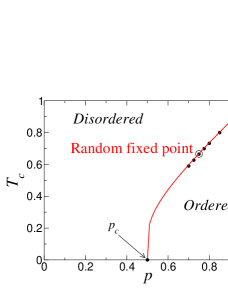
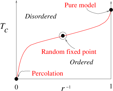
Figure 1: Phase diagram of the dilution (left) and binary problems (right).

The $q-$state Potts model [16] is the natural candidate for the investigations of influence of disorder, since the pure model exhibits two different regimes (see figure 2): a second order phase transition when $q\leq 4$ and a first order one for $q>4$ in two dimensions ($2D$). In $3D$, ordering is easier and the transition becomes weakly first-order at $q=3$ already.

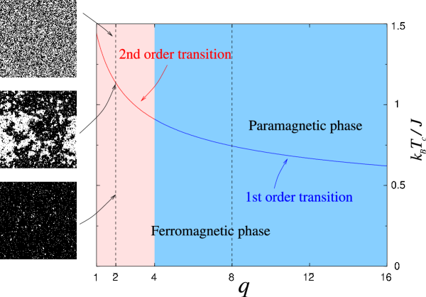
Figure 2: Phase diagram of the $2D$ pure Potts model as a function of the number of states per spin. The transition is of second-order when $q\leq 4$ and becomes of first-order above. Inserts show Monte Carlo snapshots of typical spin configurations.

The 2-dimensional $q$-state Potts model is defined by the following Hamiltonian :

$$-\beta{\cal H}=\sum_{(i,j)}K_{ij}\delta_{\sigma_{i},\sigma_{j}}$$ (5)

where the sum is restricted to nearest neighbours (here on a square lattice), the degrees of freedom $\{\sigma_{i}\}$ can take $q$ values and the exchange couplings $K_{ij}=J_{ij}/k_{B}T$ are quenched independent random variables chosen according to some distribution $\{K_{ij}\}$ to be specified later.

Many results were obtained for quenched randomness in this model in the last ten years, including

i)

perturbative expansions for $2\leq q\leq 4$ [17, 18, 19, 20, 21, 22, 23, 24, 25, 26, 27]. This work was initiated in a series of papers by A.W.W. Ludwig and J.L. Cardy [17, 18, 19]. A systematic study of energy-energy and spin-spin correlators in random bond Ising and Potts models, including tests of replica symmetry, was then performed by a group around Vl.S. Dotsenko [20, 21, 22, 23, 24, 25, 26], with M. Picco, P. Pujol, Vik. Dotsenko, J.L. Jacobsen, and M.-A. Lewis.

ii)

Monte Carlo simulations in both regimes $2\leq q\leq 4$ and $q>4$ [28, 29, 30, 31, 32, 33, 34, 35]. In the second order regime, simulations were first performed by S. Wiseman and E. Domany in the case of the Ashkin-Teller model [36] (which exhibits a critical line and for a given set of couplings belongs to the $4-$state Potts model universality class) and in the $3-$state Potts model by J.K. Kim [37]. In the case $q=8$, the first Monte Carlo simulations were reported by S. Chen, A.M. Ferrenberg and D.P. Landau in Refs. [38, 39], but then in both regimes, more accurate results were obtained by different groups, like M. Picco [28], T. Olson and P. Young [34], or the present authors [29, 30].

iii)

Transfer matrices in both regimes [40, 41, 42, 43, 44, 45, 46, 47, 48]. This technique was used to study random Potts models very early by U. Glaus, then more refined computations were reported, for example by J.L. Cardy and J.L. Jacobsen [41, 43] or in Ref. [46].

iv)

High-temperature series expansions, initially used in the random Ising model [49, 50] to show the logarithmic corrections, then extended at $q=3$ in $3D$ [51, 52], were also shortly applied to the two-dimensional case [53].

v)

Short-time dynamic scaling [54, 55, 56, 57, 58].

We also notice that dynamical properties (in order to discriminate between conventional or activated dynamics) linked to non self-averaging have been recently studied also [59] and that the interesting limit $q\to\infty$ was carefully investigated in Refs. [45, 60]. Reviews on selective parts of the subject were reported in Ph.D dissertations in Refs. [61, 62, 63, 64, 65].

Although closely related, the random-bond Ising model will not be discussed here, since it was already the subject of many reviews, e.g. [66, 67, 68]. We will only remind here that in the pure $2D$ Ising model, the exponent $\alpha$ of the specific heat vanishes and further investigation is needed, since the Harris criterion becomes inconclusive. It is now generally believed that uncorrelated quenched randomness is a marginally irrelevant perturbation which does not modify the universal critical behaviour, but produces logarithmic corrections. For example the singular part of the specific heat exhibits the following behaviour,

$$C_{s}(t)\sim\ln(1/{|t|})\qquad \theta\ll{|t|}\ll 1,$$

$$C_{s}(t)\sim\ln\ln(1/{|t|})\quad {|t|}\ll\theta,$$

$$\theta\sim{\rm e}^{-\pi/g^{2}},$$

where $g$ is the amplitude of disorder, linked to the impurity concentration. The behaviour of the main physical quantities in the neighbourhood of the random fixed point is given in table 1. It was confirmed unambiguously by Monte Carlo simulations [69, 70, 71, 72] as shown in the same table. We also note that conformal mappings associated to Monte Carlo simulations were initially used in the random-bond Ising problem by A. Talapov and Vl.S. Dotsenko [73].

Random-bond Ising model
	analytical results	numerical results
Correlation function	$\langle\sigma_{0}\sigma_{R}\rangle\sim R^{-1/4}(\ln R)^{1/8}$	$\eta=0.2493\pm 0.0014$
Correlation length	$\xi(t)\sim{|t|}^{-1}[\ln(1/{|t|})]^{1/2}$
Magnetisation	$m(t)\sim{|t|}^{1/8}[\ln(1/{|t|})]^{1/16}$	${\beta}/{\nu}=0.1245\pm 0.0009$
Susceptibility	$\chi(t)\sim{|t|}^{-7/4}[\ln(1/{|t|})]^{7/8}$	${\gamma}/{\nu}=1.7507\pm 0.0014$
Specific heat	$C(t)\sim\ln\ln(1/{|t|})$

Table 1: Critical behaviour of the random-bond Ising model.

The numerical studies of disordered models showed that many difficulties, like the lack of self averaging [74, 75, 76, 77] or varying effective exponents due to crossover phenomena. Averaging physical quantities over the samples with a poor statistics may thus lead to erroneous determinations of the critical exponents. Almost all the studies mentioned here were reported in the case of the random bond system with self-dual probability distributions of the coupling strengths in order to preserve the exact knowledge of the transition line, which is an important simplification when one wants to use finite-size-scaling techniques or conformal mappings which hold at criticality only.

In real experiments on the other hand, disorder is inherent to the working-out process and may result e.g. from the presence of impurities or vacancies. For the description of such a disordered system, dilution is thus more realistic than for example a random distribution of non-vanishing couplings (the so-called random-bond problem). Since universality is expected to hold, the detailed structure of the Hamiltonian should not play any determining role in universal quantities like critical exponents, but crossover phenomena may alter the determination of the universality class. Experimentally, the role of disorder in $2D$ systems has been investigated in several systems. Illustrating the influence of random defects in the case of the $2D$ Ising model universality class, samples made of thin magnetic amorphous layers of (Tb_0.27Dy_0.73)_0.32Fe_0.68 of 10 Å  width, separated by non magnetic spacers of 100 Å  Nb in order to decouple the magnetic layers were produced using sputtering techniques. A structural analysis (high resolution transmission electron microscopy and $x$-ray analysis) was performed to characterise the defects inherent to such amorphous structures, and in spite of these random defects separated on average by a distance of a few nm, the samples were shown to exhibit Ising-like singularities with critical exponents [78]

$$\beta=0.126(20),\ \gamma=1.75(3),\ \delta=15.1(10).$$

This is coherent with the fact that disorder does not change the universality class of the $2D$ Ising model, apart from logarithmic corrections which are probably impossible to observe experimentally, since their role becomes prominent only in the very neighbourhood of the critical point. A beautiful experimental confirmation of the Harris criterion – which predicts a modification of the critical behaviour in random systems when the exponent $\alpha$ of the specific heat is positive for the pure system – was reported in a Low Energy Electron Diffraction investigation of a $2D$ order disorder transition [79] belonging to the 4-state Potts model universality class. Order-disorder transitions of adsorbed atomic layers are known to belong to different two-dimensional universality classes depending on the type of superstructures in the ordered phase of the ad-layer [80, 81]. The substrate plays a major role in ad-atom ordering, as well as the coverage (defined as the number of ad-atoms per surface atom) which determines the possible superstructures of the over-layer. For example, sulfur chemisorbed on Ru$(001)$ exhibits four-state or three-state Potts critical singularities for the $p(2\times 2)$ and the $(\sqrt{3}\times\sqrt{3})R30^{\circ}$ respectively [82] (at coverages $1/4$ and $1/2$). The case of the $(2\times 2)-$2H/Ni$(111)$ order-disorder transition of hydrogen adsorbed on the $(111)$ surface of Ni thus belongs to the $2D$ four-state Potts model universality class, since the ground state, stable at low temperatures, has a four-fold degenaracy due to the four possible coverings of the ad-atoms at the $(111)$ surface (see figure 3).

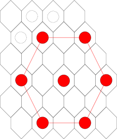
Figure 3: $(2\times 2)-$2H/Ni$(111)$ order-disorder transition of hydrogen. The ground-state has a four-fold degenaracy due to the four possible covering of the $(111)$ surface of Ni by H ad-atoms.

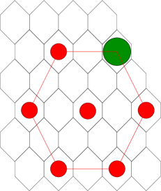
Figure 4: $(2\times 2)-$2H/Ni$(111)$ order-disorder transition of hydrogen with oxygen impurities randomly chemisorbed on the surface, and occupying some of the lattice sites.

The expected exponents are thus close to theoretical values of $\beta=1/12\simeq 0.083$, $\gamma=7/6\simeq 1.167$, and $\nu=2/3\simeq 0.667$ for example.

Low energy electron diffraction (LEED) makes possible to measure these exponents through the diffracted intensity $I({\bf q})$ or structure factor. This is the two-dimensional Fourier transform of the pair correlation function of ad-atom density. Long range fluctuations produce an isotropic Lorentzian centered at the superstructure spot position ${\bf q}_{0}$ with a peak intensity given by the susceptibility and a width determined by the inverse correlation length, while long range order gives a background signal proportional to the order parameter squared:

$$I({\bf q})=\langle m^{2}\rangle\delta({\bf q}-{\bf q}_{0})+\frac{\chi}{1+\xi^{2}({\bf q}-{\bf q}_{0})^{2}}.$$

The following exponents were thus measured [79, 83, 84]

$$\beta=0.11\pm 0.01,\ \gamma=1.2\pm 0.1,\ \nu=0.68\pm 0.05$$

in correct agreement with 4-state Potts values (the small deviation, especially for the exponent $\beta$, is attributed to the logarithmic corrections to scaling of the pure 4-state Potts model [85]). The same experiments were then reproduced in the presence of intentionally added oxygen impurities, at a temperature which is above the ordering temperature of pure oxygen adsorbed on the same substrate. The mobility of these oxygen atoms is furthermore considered to be low enough at the hydrogen order-disorder transition critical temperature that they essentially represent quenched impurities randomly distributed in the hydrogen layer (see figure 4). The exponents become

$$\beta=0.135\pm 0.010,\ \gamma=1.68\pm 0.15,\ \nu=1.03\pm 0.08,$$

which definitely supports the modification of the universality class in the presence of quenched disorder, in agreement with Harris criterion ($\alpha=2/3$ for the 4-state Potts model).

The aim of this lecture is to provide a review of both perturbative and numerical studies of the bond diluted Potts model for several values of the number of states per spin (in order to cover the two different regimes of the pure system’s phase transitions). In section 2, the perturbative approach is discussed and the essential results are summarised in the $2D$ case with $2\leq q\leq 4$. The details of the numerical techniques used in two dimensions are presented in section 3 and  4, while the comparison between numerical and analytical results is made in  5.

2 Perturbative approach in $2D$

2.1 Replicas and relevance criterion

For a specific disorder realization $[K_{ij}]$, the Hamiltonian ${\cal H}[K_{ij},\sigma_{i}]$ is written

$$-\beta{\cal H}[K_{ij},\sigma_{i}]=\sum_{(ij)}(K_{0}+\delta K_{ij})\delta_{\sigma_{i},\sigma_{j}}.$$ (6)

The corresponding partition function and free energy are given as follows

$$Z[K_{ij}]=\int{\cal D}[\sigma_{i}]{\rm e}^{-\beta{\cal H}[K_{ij},\sigma_{i}]},$$

$$F[K_{ij}]=-k_{B}T\ln Z[K_{ij}].$$

To get the quantities of interest, for example the average free energy, we have to perform an average over the distribution ${\cal P}[K_{ij}]$,

$$F=\overline{F[K_{ij}]}=-k_{B}T\int{\cal D}[K_{ij}]{\cal P}[K_{ij}]\ln Z[K_{ij}].$$ (7)

Averaging the logarithm of the partition function is possible through the identity

$$\ln Z=\lim_{n\to\infty}\frac{1}{n}(Z^{n}-1),$$

which requires, before averaging, to produce $n$ copies (with labels $\alpha$) of the system with the same disorder configuration,

$$(Z[K_{ij}])^{n}=\int\left(\prod_{\alpha=1}^{n}{\cal D}[{\sigma}^{(\alpha)}_{i}]\right){\rm e}^{-\beta\sum_{\alpha}{\cal H}[K_{ij},{\sigma}^{(\alpha)}_{i}]},$$

and then to perform integrations over ${\cal P}[K_{ij}]$,

$$\overline{{\rm e}^{-X}}={\rm e}^{-\bar{X}+\frac{1}{2}(\overline{X^{2}}-\bar{X}^{2})+\dots},$$

leading to

$$\overline{(Z[K_{ij}])^{n}} = \int\left(\prod_{\alpha=1}^{n}{\cal D}[{\sigma}^{(\alpha)}_{i}]\right){\rm e}^{-\sum_{\alpha}(K_{0}+\overline{\delta K})\sum_{(ij)}\delta_{\sigma_{i}^{(\alpha)},\sigma_{j}^{(\alpha)}}}$$ (8)

$$\times{\rm e}^{\sum_{\alpha\not=\beta}(\overline{\delta K^{2}}-\overline{\delta K}^{2})\sum_{(ij)}\delta_{\sigma_{i}^{(\alpha)},\sigma_{j}^{(\alpha)}}\delta_{\sigma_{i}^{(\beta)},\sigma_{j}^{(\beta)}}+\dots}$$

In the leading term, $\overline{\delta K_{ij}}$ has RG eigenvalue $y_{t}=d-x_{\varepsilon}$ and corresponds to a simple shift of the transition 4 temperature (which is obviously a relevant effect). In the next term, the second moment of the distribution, $\overline{\delta K^{2}}-\overline{\delta K}^{2}$, has RG eigenvalue $y_{H}=d-2x_{\varepsilon}$, and all the following terms are irrelevant. Using hyperscaling relation, the Harris scaling dimension of disorder is rewritten

$$y_{H}=\alpha/\nu.$$ (9)

It implies that at second-order transitions, disorder is a relevant perturbation which modifies the critical behaviour when the specific heat exponent $\alpha$ of the pure system is positive, while it is irrelevant (and universal properties are thus unaffected by randomness) when $\alpha$ is negative. In the borderline case $\alpha=0$, randomness is marginal to leading order. This is the case for example of the $2D$ Ising model discussed in the introduction, where quenched disorder is eventually marginally irrelevant and produces only logarithmic corrections to the unchanged leading critical behaviour.

The case of first-order transitions was considered later, by Imry and Wortis, Aizenman and Wehr, then Hui and Berker [2, 3, 4]. It can be intuitively understood from the above results simply by noticing that the existence of a latent heat at first-order transition corresponds to a discontinuity of the energy density and can be described by a vanishing energy density scaling dimension, so that disorder is always relevant in this sense.

2.2 Perturbation techniques

2.2.1 Average correlation functions

Many results were obtained in the $2D$ random Potts model using RG perturbations, mainly around Ludwig and Vl. Dotsenko. In equation (8), it appears that $\overline{Z^{n}}$ couples the replicas via energy-energy interactions $\sum_{\alpha\not=\beta}(\overline{\delta K^{2}}-\overline{\delta K}^{2})\sum_{\bf r}\varepsilon_{\alpha}({\bf r})\varepsilon_{\beta}({\bf r})$ which have to be treated as a perturbation around the pure fixed point. Here, $\varepsilon_{\alpha}({\bf r})$ is a short notation for $\delta_{\sigma_{i}^{(\alpha)}\sigma_{j}^{(\alpha)}}$, and ${\bf r}$ stands for the lattice unit vectors. The second cumulant of the coupling distribution will be denoted $g_{0}$ in the following. Two different schemes were considered in the literature [25, 61],

i)

replica symmetric scenario, where all the replicas are coupled through the same interaction strength,

$$\sum_{\alpha\not=\beta}g_{0}\sum_{\bf r}\varepsilon_{\alpha}({\bf r})\varepsilon_{\beta}({\bf r}),$$ (10)

ii)

replica symmetry breaking scenario, where the coupling between replicas are replica-dependent,

$$\sum_{\alpha\not=\beta}g_{\alpha\beta}\sum_{\bf r}\varepsilon_{\alpha}({\bf r})\varepsilon_{\beta}({\bf r}).$$ (11)

The program is thus to consider $2D$ Potts model with weak bond randomness, compute the scaling dimensions $x^{\prime}_{\sigma}(n)$ of the order parameter and $x^{\prime}_{\varepsilon}(n)$ of the energy-density perturbatively around the Ising model conformal field theory, and then take the replica limit $n\to 0$. Expansions are performed around the pure model fixed point (weak disorder) in terms of the disorder strength $\overline{\delta K_{ij}^{2}}-\overline{\delta K_{ij}}^{2}$, and the exponents are given in powers of $y_{H}=\alpha/\nu$.

Different expansion parameters can be found in the literature, and it is worth collecting the main notations. The Potts models can be identified to minimal conformal models [87] which are parametrised by an integer $m$ which determines the central charge and critical behaviour of the model. The correspondence is given by

$$m=\frac{\pi}{\cos^{-1}(\sqrt{q}/2)}-1$$

and the central charge and exponents follow from

$$c = 1-\frac{6}{m(m+1)},$$

$$x_{\varepsilon} = \frac{m+3}{2m},$$

$$x_{\sigma} = \frac{(m+3)(m-1)}{8m(m+1)}.$$

We note that $m=3$ for the Ising model, $m=5$ for the $3-$state Potts model and $m\to\infty$ for the $4-$state Potts model. The Harris RG eigenvalue becomes

$$y_{H}=\frac{m-3}{m},$$

which is proportional to $q-2$ to linear order ($q$ being the number of states per spin of the Potts model):

$$y_{H}=\frac{4}{3\pi}(q-2)-\frac{4}{9\pi^{2}}(q-2)^{2}+O[(q-2)^{3}].$$ (12)

Using a Coulomb gas representation, a natural expansion parameter $\epsilon$ is defined through

$$\alpha_{+}^{2}=\frac{m+1}{m}=\frac{4}{3}+\epsilon,$$

and it is linked to $y_{H}$ by $\epsilon=-\frac{1}{3}y_{H}$.

i)

The replica symmetric case is based on the assumption that replica symmetry is not broken initially, and is then preserved by the renormalization group. The renormalization of the coupling constant $g_{0}$ is determined by perturbative calculation using the operator algebra. For any scaling operator $\phi$, the perturbed two-point correlation function $\langle\phi(0)\phi({\bf R})\rangle_{g}$ corresponds, in the limit $n\to 0$, to the average correlator $\overline{\langle\phi(0)\phi({\bf R})\rangle}$. We can write

$$\langle\phi(0)\phi({\bf R})\rangle_{g}=\frac{{\rm Tr}{\ \!\phi(0)\phi({\bf R})\rm e}^{-\beta({\cal H}_{c}+{\cal H}_{g})}}{{\rm Tr}{\ \!\rm e}^{-\beta({\cal H}_{c}+{\cal H}_{g})}}$$

where the perturbation term $-\beta{\cal H}_{g}=g_{0}\int\sum_{\alpha\not=\beta}\varepsilon_{\alpha}({\bf r})\varepsilon_{\beta}({\bf r}){\rm d}^{2}r$ acts on the ‘critical’ Hamiltonian $-\beta{\cal H}_{c}=m_{0}\int\sum_{\alpha}\varepsilon_{\alpha}({\bf r}){\rm d}^{2}r+h_{0}\int\sum_{\alpha}\sigma_{\alpha}({\bf r}){\rm d}^{2}r$, the last term being included in order to compute the renormalization of the spin operator.

When expanded in terms of unperturbed correlators, it yields the following expansion [88, 89]

$$\langle\phi(0)\phi({\bf R})\rangle_{g} = \langle\phi(0)\phi({\bf R})\rangle_{0}-\beta\langle{\cal H}_{g}\phi(0)\phi({\bf R})\rangle_{0}$$

$$+\frac{1}{2}\beta^{2}\langle{\cal H}_{g}^{2}\phi(0)\phi({\bf R})\rangle_{0}+\dots$$

The renormalization of the coupling constant follows from the expansion [20, 21, 22, 23]

$$g_{0}\int\sum_{\alpha\not=\beta}\varepsilon_{\alpha}({\bf r})\varepsilon_{\beta}({\bf r}){\rm d}^{2}r$$

$$+\frac{1}{2}g_{0}^{2}\int\sum_{\alpha\not=\beta}\varepsilon_{\alpha}({\bf r})\varepsilon_{\beta}({\bf r}){\rm d}^{2}r\int\sum_{\gamma\not=\delta}\varepsilon_{\gamma}({\bf r}^{\prime})\varepsilon_{\delta}({\bf r}^{\prime}){\rm d}^{2}r^{\prime}+\dots$$

$$=g\int\sum_{\alpha\not=\beta}\varepsilon_{\alpha}({\bf r})\varepsilon_{\beta}({\bf r}){\rm d}^{2}r,$$ (13)

leading to $g=g_{0}(1+A_{1}g_{0}+A_{2}g_{0}^{2}+\dots)$. The successive terms are obtained from operator product expansions. In the first order term, the dominant contribution to $A_{1}$ follows from contraction of neighbouring pairs, $\varepsilon({\bf r})\varepsilon({\bf r}^{\prime})\sim|{\bf r}-{\bf r}^{\prime}|^{-2x_{\varepsilon}}$, in the same replica ($\beta=\gamma\not=\alpha,\delta$ and $\alpha\not=\delta$). Such an expression has to be understood inside unperturbed correlators. Including combinatorial factors (they are $2(n-2)$ such factors), integration over space up to an infrared cutoff, $b>|{\bf r}-{\bf r}^{\prime}|$, leads to $\frac{1}{2}g_{0}^{2}A_{1}\int\sum_{\alpha\not=\delta}\varepsilon_{\alpha}({\bf r})\varepsilon_{\delta}({\bf r}){\rm d}^{2}r$, where $A_{1}$ is dominated by

$$A_{1}=2(n-2)\int_{|{\bf r}-{\bf r}^{\prime}|<b}|{\bf r}-{\bf r}^{\prime}|^{-2x_{\varepsilon}}{\rm d}^{2}r^{\prime}=4\pi(n-2)\frac{b^{2-2x_{\varepsilon}}}{2-2x_{\varepsilon}}.$$

Since $y_{H}=2-2x_{\varepsilon}$, one recovers the Harris criterion. Up to the first order, we get the following expression for $g$ in terms of the bare coupling constant $g_{0}$, $g=g_{0}(1+2\pi(n-2)\frac{1}{y_{H}}b^{y_{H}}g_{0}+\mathop{O}\nolimits(g_{0}^{2}))$. Following Dotsenko and co-workers, the coupling constants are multiplied by a factor $b^{y_{H}}$ in order to get dimensionless coupling constants $g(b)$.

The $\beta-$function up to second order in the $n\to 0$ limit is finally given by

$$\beta(g)=\frac{{\rm d}g(b)}{{\rm d}\ln b}=y_{H}g(b)-8\pi g^{2}(b)+32\pi^{2}g^{3}(b)+\mathop{O}\nolimits(g^{4}(b)).$$ (14)

It leads to a non trivial IR fixed point (which determines the long distance physics) $g_{c}=\frac{1}{8\pi}y_{H}+\frac{1}{16\pi}y_{H}^{2}+\mathop{O}\nolimits(y_{H}^{3})$.

Renormalization of the energy and the order parameter density operators follow from the same analysis, e.g.:

$$m_{0}\int\sum_{\alpha}\varepsilon_{\alpha}({\bf r}){\rm d}^{2}r\left(1+g_{0}\int\sum_{\beta\not=\gamma}\varepsilon_{\beta}({\bf r}^{\prime})\varepsilon_{\gamma}({\bf r}^{\prime}){\rm d}^{2}r^{\prime}\right.$$

$$\left.+\frac{1}{2}g_{0}^{2}\int\sum_{\beta\not=\gamma}\varepsilon_{\beta}({\bf r}^{\prime})\varepsilon_{\gamma}({\bf r}^{\prime}){\rm d}^{2}r^{\prime}\int\sum_{\delta\not=\eta}\varepsilon_{\delta}({\bf r}^{\prime\prime})\varepsilon_{\eta}({\bf r}^{\prime\prime}){\rm d}^{2}r^{\prime\prime}+\dots\right)$$

$$=m\int\sum_{\alpha}\varepsilon_{\alpha}({\bf r}){\rm d}^{2}r,$$ (15)

and provide the expansions (details of the calculation of the integrals, using a Coulomb gas representation, can be found e.g. in Ref. [20]) $m=m_{0}(1+B_{1}g_{0}+B_{2}g_{0}^{2}+\dots)=Z_{\varepsilon}m_{0}$ and $h=h_{0}(1+C_{1}g_{0}+C_{2}g_{0}^{2}+\dots)=Z_{\sigma}h_{0}$, leading when $n\to 0$ to

$$\gamma_{\varepsilon}(g) = \frac{{\rm d}\ln Z_{\varepsilon}}{{\rm d}\ln b}=-4\pi g(b)+8\pi^{2}g^{2}(b),$$

$$\gamma_{\sigma}(g) = \frac{{\rm d}\ln Z_{\sigma}}{{\rm d}\ln b}=-\pi^{2}y_{H}g^{2}(b)\left(1+2\frac{\Gamma^{2}(-{\scriptstyle\frac{2}{3}})\Gamma^{2}({\scriptstyle\frac{1}{6}})}{\Gamma^{2}(-{\scriptstyle\frac{1}{3}})\Gamma^{2}(-{\scriptstyle\frac{1}{6}})}\right)+8\pi^{2}g^{3}(b).$$

For the correlators themselves, the renormalization equations can be written

$$\langle\phi(0)\phi(s{\bf R})\rangle=\frac{Z^{2}_{\phi}(g(bs))}{Z^{2}_{\phi}(g(b))}s^{-2x_{\phi}}\langle\phi(0)\phi({\bf R})\rangle,$$

where $s$ is the scaling factor. Using now

$$\gamma_{\phi}(g)=\frac{{\rm d}\ln Z_{\phi}}{{\rm d}\ln b},$$

or $\ln Z_{\phi}=\int\gamma_{\phi}(g){\rm d}\ln b$, the ratio $\frac{Z^{2}_{\phi}(g(bs))}{Z^{2}_{\phi}(g(b))}$ can be rewritten

$$\frac{Z_{\phi}^{2}(bs)}{Z_{\phi}^{2}(b)}={\rm e}^{2\int_{b}^{bs}\gamma_{\phi}(g){\rm d}\ln b}$$

which is dominated at long distances by $g\simeq g_{c}$, such that $\int_{b}^{bs}\gamma_{\phi}(g){\rm d}\ln b\simeq\gamma_{\phi}(g_{c})\ln s$. The homogeneity equation thus becomes

$$\langle\phi(0)\phi(s{\bf R})\rangle=s^{-2(x_{\phi}-\gamma_{\phi}(g_{c}))}\langle\phi(0)\phi({\bf R})\rangle,$$

and choosing a rescaling factor $s=R^{-1}$, the two point correlator decays as

$$\langle\phi(0)\phi({\bf R})\rangle\simeq R^{-2(x_{\phi}-\gamma_{\phi}(g_{c}))}.$$ (17)

The corresponding scaling dimension is modified according to

$$x^{\prime}_{\phi}=x_{\phi}-\gamma_{\phi}(g_{c}).$$ (18)

Collecting the results of Dotsenko and co-workers, we give the new thermal and magnetic scaling dimensions (with primes) in terms of the original ones (unprimed) [20, 21, 22, 23]:

$$x^{\prime}_{\varepsilon} = x_{\varepsilon}-\gamma_{\varepsilon}(g_{c})$$ (19)

$$= x_{\varepsilon}+\frac{1}{2}y_{H}+\frac{1}{8}y_{H}^{2}+\mathop{O}\nolimits(y_{H}^{3})$$

$$x^{\prime}_{\sigma} = x_{\sigma}-\gamma_{\sigma}(g_{c})$$ (20)

$$= x_{\sigma}+\frac{1}{32}\frac{\Gamma^{2}(-{\scriptstyle\frac{2}{3}})\Gamma^{2}({\scriptstyle\frac{1}{6}})}{\Gamma^{2}(-{\scriptstyle\frac{1}{3}})\Gamma^{2}(-{\scriptstyle\frac{1}{6}})}y_{H}^{3}+\mathop{O}\nolimits(y_{H}^{4})$$

ii)

The other assumption of a broken replica symmetry leads to a different fixed point structure. The coupling between replicas, $g_{\alpha\beta}$, is now dependent on the pair indexes, and it is generalised to a continuous variable $x$ instead of pair indices, $g_{\alpha\beta}\to g(\alpha-\beta)=g(x)$. It is found that there is only one marginally attractive solution for the coupling $g(x)$ which then enable to compute $\gamma_{\varepsilon}(g)$ and $\gamma_{\sigma}(g)$, leading to a modified thermal exponent

$$x^{\prime\prime}_{\varepsilon}=x_{\varepsilon}+\frac{1}{2}y_{H}+\mathop{O}\nolimits(y_{H}^{3}),$$ (21)

while to $y_{H}^{3}$ order, the magnetic scaling index remains the same as in the replica symmetric scenario [22].

2.2.2 Multiscaling and higher order moments of the correlators

In order to measure some other differences between the replica symmetric and the replica symmetry breaking cases, the moments of the correlators can also be helpful. For any scaling field $\phi({\bf r})$, multiscaling arises when the scaling dimensions associated to the moments of the correlators do not follow a simple linear law:

$$\overline{\langle\phi(0)\phi({\bf R})\rangle^{p}}\sim R^{-2px_{\phi^{p}}},\ x_{\phi^{p}}\not=x_{\phi}.$$ (22)

In the magnetic sector, a difference between the two cases occurs to $y_{H}^{2}$ order for the second moment [25]:

$$RS x^{\prime}_{\sigma^{2}}=x_{\sigma}-\frac{1}{16}y_{H}+\frac{1}{32}\left(4\ln 2-{\scriptstyle\frac{11}{12}}\right)y_{H}^{2}+\mathop{O}\nolimits(y_{H}^{3}),$$ (23)

$$RSB x^{\prime\prime}_{\sigma^{2}}=x_{\sigma}-\frac{1}{16}y_{H}+\frac{1}{32}\left(4\ln 2-{\scriptstyle\frac{5}{12}}\right)y_{H}^{2}+\mathop{O}\nolimits(y_{H}^{3}).$$ (24)

For higher order moments, the computation were only performed in the replica symmetric case [19, 26, 27], leading to

$$x^{\prime}_{\varepsilon^{p}} = 1-\frac{2}{9\pi^{2}}(3p-4)(q-2)^{2}+O[(q-2)^{3}],$$ (25)

$$x^{\prime}_{\sigma^{p}} = 1-\frac{1}{16}(p-1)y_{H}^{2}$$ (26)

$$-\frac{1}{32}(p-1)[{\scriptstyle\frac{11}{12}-4\ln 2+\frac{1}{24}(33-29\sqrt{3}\pi/3)(p-2)}]y_{H}^{3}+\mathop{O}\nolimits(y_{H}^{4}).$$

2.2.3 Are these effects measurable?

The question is now to try to detect numerically the effects discussed above. These are perturbative expansions around $q=2$, so that a natural choice of system to measure the scaling dimensions in the presence of quenched disorder is the $3-$state Potts model. At $q=3$ we have $x_{\varepsilon}=4/5$ and $y_{H}=2/5$ from which the perturbed scaling dimensions in the energy and magnetic sectors can be obtained. The values are given in table 2. The numerical data clearly show that the expected variations are quite small and need accurate numerical techniques to discriminate between RS and RSB schemes.

Scheme	Scaling dimensions
	$x_{\sigma}$	$x_{\varepsilon}$	$x_{\sigma^{2}}$	$x_{\sigma^{0}}$	$x_{\varepsilon^{0}}$
Pure system	0.13333	0.800	0.13333	0.13333	0.800
RS	0.13465	1.000	0.11761	0.18303	1.090
RSB	0.13465	1.020	0.12011	–	–

Table 2: Comparison between pure $3-$state Potts model critical exponents and the expected values obtained from perturbation expansions. The notation $x_{\sigma^{2}}$ corresponds to the second moment of the spin-spin correlation function, while $x_{\sigma^{0}}$ and $x_{\varepsilon^{0}}$ are associated to the typical correlations.

3 Numerical techniques in $2D$

3.1 Monte Carlo simulations

3.1.1 Cluster algorithms

For the simulation of spin systems, standard Metropolis algorithms based on local updates of single spins suffer from the well known critical slowing down. As the second-order phase transition is approached, the correlation length becomes larger and the system contains larger and larger clusters in which all the spins are in the same state. Statistically independent configurations can be obtained by local iteration rules only after a long dynamical evolution which needs a huge number of MC steps. This makes this type of algorithm inefficient close to a critical point.

Since the transition of the disordered Potts model is always expected to be on average a second-order one, the resort to cluster update algorithms is more convenient [90, 91]. The main recipe of cluster algorithms is the identification of clusters of sites using a bond percolation process connected to the spin configuration. The spins of the clusters are then independently flipped. A cluster algorithm is particularly efficient if the percolation threshold coincides with the transition point of the spin model, which guarantees that clusters of all sizes will be updated in a single MC sweep.

In the case of the Potts model, the percolation process involved is obtained through the mapping onto the random graph model. These algorithms are based on the Fortuin-Kasteleyn representation [92] where bond variables are introduced. In the Swendsen-Wang algorithm [93], a cluster update sweep consists of three steps: depending on the nearest neighbour exchange interactions, assign values to the bond variables, then identify clusters of spins connected by active bonds, and eventually assign a random value to all the spins in a given cluster. The Wolff algorithm [94] is a simpler variant in which only a single cluster is flipped at a time. A spin is randomly chosen, then the cluster connected with this spin is constructed and all the spins in the cluster are updated.

Both algorithms considerably improve the efficiency close to the critical point and their performances are comparable in two dimensions, so in principle one can equally choose either one of them. Nevertheless, when one uses particular boundary conditions, with fixed spins along some surface for example, the Wolff algorithm is less efficient, since close to criticality the unique cluster will often reach the boundary and no update is made in this case.

3.1.2 Definition of the physical quantities

For each disorder strength, many samples ($N_{\rm rdm}$) from the same probability distribution are studied at a given temperature. Each sample, initialised from the low-temperature phase, is thermalized during $N_{\rm th}$ Monte Carlo sweeps and the physical quantities are then measured during $N_{\rm MC}$ sweeps. Different quantities, averaged over the MC sweeps denoted by $\langle\dots\rangle$, are conserved for all the samples. Many physical quantities can be measured:

1. The order parameter density follows from the standard definition for the Potts model:

   $$M=\langle\sigma\rangle,\quad\sigma=\frac{q\rho_{\rm max}-1}{q-1},$$

   where $\rho_{\rm max}$ is the fraction of spins in the majority orientation

   $$\rho_{\rm max}={\rm Max}_{\alpha}(\rho_{\alpha}),\quad\rho_{\alpha}=\frac{1}{L^{2}}\sum_{j}\delta_{\sigma_{j},\alpha}.$$

   Thermal average is understood in the notation $M$. To obtain the local order parameter $\langle\sigma(i)\rangle$ at site $i$, it is counted 1 when the spin at site $i$ is in the majority state and 0 otherwise.

2. The susceptibility is given by fluctuation-dissipation theorem

   $$k_{B}T\chi=\langle\sigma^{2}\rangle-\langle\sigma\rangle^{2}.$$

3. Energy density:

   $$E=\langle\varepsilon\rangle,\quad\varepsilon=\frac{1}{2L^{2}}\sum_{(i,j)}K_{ij}\delta_{\sigma_{i},\sigma_{j}}.$$

4. Specific heat:

   $$C/k_{B}=\langle\varepsilon^{2}\rangle-\langle\varepsilon\rangle^{2}.$$

5. Energy Binder cumulant:

   $$U_{E}=1-\frac{\langle\varepsilon^{4}\rangle}{3\langle\varepsilon^{2}\rangle^{2}}.$$

6. Correlation functions: the connected spin spin correlation function $G_{\sigma}(i,j)=\langle\sigma(i)\sigma(j)\rangle-\langle\sigma^{2}\rangle$ at criticality is obtained by the estimator of the paramagnetic phase,

   $$\frac{q\langle\delta_{\sigma_{i}\sigma_{j}}\rangle-1}{q-1},$$

   given by the probability that spins at sites $i$ and $j$ belong to the same finite cluster.

All these quantities are then averaged over the disorder realisations

$$\overline{\langle...\rangle}=\int\langle...\rangle{\cal P}[\langle...\rangle]{\rm d}\langle...\rangle.$$

3.2 Transfer matrix technique

The disordered Potts model can be studied using the transfer matrix method introduced by Blöte and Nightingale [95], which takes advantage of the Fortuin-Kasteleyn representation [92] in terms of graphs of the partition function of the Potts model in order to reduce the dimension of the Hilbert space . In the Fortuin-Kasteleyn representation, the partition function (with no magnetic field) is

$$Z={\rm Tr}\prod_{(i,j)}(1+\delta_{\sigma_{i},\sigma_{j}}u_{ij}),$$

where $u_{ij}={\rm e}^{K_{ij}}-1$, is expanded as a sum over all the possible graphs ${\cal G}$ (with $s$ sites and $l({\cal G})$ loops) leading to the random cluster model:

$$Z=q^{s}\sum_{\cal G}q^{l({\cal G})}\prod_{(i,j)/b_{ij}=1}\left(\frac{u_{ij}}{q}\right),$$

$b_{ij}\in\{0;1\}$ being the bond variables. Blöte and Nightingale suggested to introduce a set of connectivity states which contain the information about which sites on a given row belong to the same cluster when they are interconnected through a part of the lattice previously built. A unique connectivity label $\eta_{i}=\eta$ is attributed to all the sites $i$ of such a cluster. In the connectivity space, $|Z(m)\rangle$ is a vector whose components are given by the partial partition function $Z(m,\{\eta_{i}\}_{m})$ of a strip of length $m$ whose connectivity on the last row is given by $\{\eta_{i}\}_{m}$. The connectivity transfer matrix is then defined according to $|Z(m+1)\rangle={\bf T}_{m}|Z(m)\rangle$ and the partition function of a strip of length $m$ becomes $|Z(m)\rangle=\prod_{k=1}^{m-1}{\bf T}_{k}|Z(1)\rangle$, where $|Z(1)\rangle$ is the statistics of uncorrelated spins.

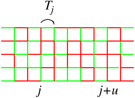
Figure 5: Transfer matrix along the disordered strip.

The following physical quantities are measured:

1. The quenched free energy density is given (up to a $k_{B}T$ factor) by the Lyapunov exponent of the product of an infinite number of transfer matrices ${\bf T}_{k}$ [97]

   $$\overline{f_{L}}=-L^{-1}\Lambda_{0}(L).$$ (27)

   $$\Lambda_{0}(L)=\lim_{m\to\infty}\frac{1}{m}\ln\left|\!\left|\left(\prod_{k=1}^{m}{\bf T}_{k}\right)\mid\!v_{0}\rangle\right|\!\right|,$$ (28)

   where $\mid\!v_{0}\rangle$ is a unit initial vector.

   For a pure system, the central charge $c$ is defined as the universal coefficient in the lowest-order correction to scaling of the free energy density ${f_{L}}$ of a strip of width $L$:

   $${f_{L}}=f_{\infty}-{\pi c\over 6L^{2}}+\mathop{O}\nolimits\left({1\over L^{4}}\right),$$ (29)

   where the regular contribution is $f_{\infty}=\lim_{L\rightarrow+\infty}{f_{L}}$. For a disordered system, $c$ is defined in the same way from the finite-size behaviour of the quenched average free energy density $\overline{f_{L}}$, and numerically, since the strip widths available are small, we can only expect to measure effective central charges which depend on the disorder strength, $c_{\rm eff}(g)$, and which would converge towards the true value $c$ in the thermodynamic limit [45, 96].

   $$\overline{f_{L}}=f_{\infty}-{\pi c_{\rm eff}\over 6L^{2}}+a_{4}L^{-4}.$$ (30)

2. The spin-spin correlation functions in the time-direction ($u$) of the strip are calculated using an extension of the Hilbert space that allows to keep track of the connectivity with a given spin. For a specific disorder realisation, the spin-spin correlation function along the strip

   $$G_{\sigma}(u)=\frac{q\langle\delta_{\sigma_{j}\sigma_{j+u}}\rangle-1}{q-1},$$ (31)

   is given by the probability that the spins along some row, at columns $j$ and $j+u$, are in the same state and is expressed, in the absence of long-range order, in terms of a product of non-commuting transfer matrices:

   $$\langle\delta_{\sigma_{j}\sigma_{j+u}}\rangle\sim\langle\Lambda_{0}\!\mid{\bf g}_{j}\left(\prod_{k=j}^{j+u-1}{\bf T}^{\prime}_{k}\right){\bf d}_{j+u}\mid\!\Lambda_{0}\rangle,$$ (32)

   where $\mid\!\Lambda_{0}\rangle$ is the ground state eigenvector and ${\bf T}_{k}^{\prime}$ is the transfer matrix in the extended Hilbert space. The operators ${\bf g}_{j}$ and ${\bf d}_{j+u}$ realise the mapping between the two connectivity spaces. The correlations were computed on strips of varying widths and then averaged over many disorder realisations.

4 Analysis of numerical data in $2D$

4.1 Location of the random fixed point

The transition line between ordered and disordered phases in the phase diagram starts at some point corresponding to the pure system and ends at another point where the critical properties are governed by the percolation universality class. Somewhere between, the random fixed point governs the critical behaviour of quenched randomness. Although this random fixed point is attractive, its precise location is an important preliminary step. Indeed, if the assumption of the existence of a unique stable random fixed point holds, one expects that the critical behaviour is asymptotically the same as the system is moved along the transition line. However, in finite systems, one generically has to deal with strong crossover effects due to the competition between the disordered fixed point and the pure and percolation fixed points, or to corrections to scaling linked to the appearance of irrelevant scaling variables. These latter effects are generally important in random systems and the corresponding corrections to scaling can be substantially reduced when one measures the critical exponents in the regime of the random fixed point, expected to be reached at the vicinity of the maximum of the effective central charge.

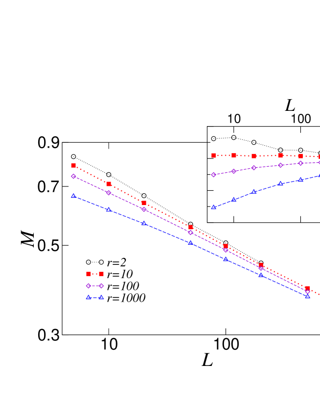
Figure 6: Finite-size scaling behaviour of the magnetisation ($q=8$, binary disorder) for different disorder amplitudes $r$ (binary distribution). The corrections to scaling are smaller close to $r=10$ (taken from Picco [28]).

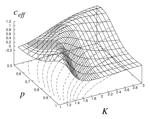
Figure 7: Dependence of the effective central charge $c_{\rm eff}$ with the exchange coupling $K$ and the bond probability $p$ for the 4-state Potts model. The maximum gives the location of the transition line and the absolute maximum corresponds to the optimal disorder strength.

Let us consider the finite-size behaviour of an observable $Q$ measured at a deviation $t=K-K_{c}(g)$ from the critical point on some system of characteristic size $L$, in the presence of disorder whose strength is measured by an amplitude $g$ (ratio $r$ between strong and weak interactions, probability $p$ of non vanishing bond,…). The variables $t$ and $L^{-1}$ play the role of relevant scaling fields (with positive RG eigenvalues $y_{t}=1/\nu$ and $y_{L}=1$ respectively), while close to the fixed point, disorder is supposed to be related to some irrelevant scaling variable with eigenvalue $y_{g}=-\omega<0$. At the fixed point there is no need that the irrelevant scaling field vanishes, so that one can write $g^{*}$ the corresponding disorder strength at the fixed point and the observable $Q$ obeys the following homogeneity assumption in the scaling region

$$Q(t,L^{-1},g)=L^{-x_{Q}}f(L^{1/\nu}t,L^{-\omega}(g-g^{*})).$$

An expansion of the last variable (keeping the leading term only) along the critical line (i.e. varying $g$ at $K_{c}(g)$) gives

$$Q(0,L^{-1},g)=\Gamma_{Q}L^{-x_{Q}}(1+\Gamma_{Q}^{(2)}(g-g^{*})L^{-\omega}+\dots),$$

where the $\Gamma$’s are non-universal critical amplitudes. It is thus possible to fix $g=g^{*}$ in order to minimise the corrections to scaling (see figure 6).

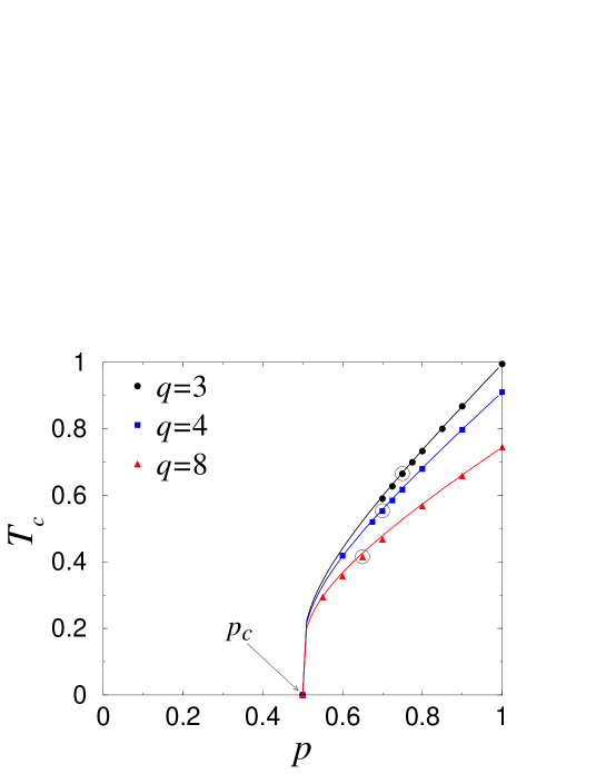
Figure 8: Phase diagram obtained from the condition of a maximum of the central charge for the dilute Potts model ($q=3$, 4, and 8). The optimal disorder strength (here $p^{*}$) is denoted by a larger circle and the full lines correspond to the single-bond effective medium approximation [100, 101, 102].

From a finite-size scaling analysis (see section 4.3), the optimal disorder strength $g^{*}$ is reached when a given quantity seems to be well fitted by a simple power-law (i.e. no bending in the the log-log plot). In the strip geometry, this value $g^{*}$ is found to coincide with the location of the maximum of the central charge along the critical line [43, 44], as a consequence of Zamolodchikov’s $c-$theorem [98] (see figure 7).

In the literature, different types of disorder distributions have been considered. In the most studied case, when self-duality holds, the exact transition curve is known and the optimal disorder strength $g^{*}$ has to be found while moving one parameter only, which simplifies the task. If one defines the variables $y_{ij}$ by ${\rm e}^{y_{ij}}=\frac{1}{\sqrt{q}}({\rm e}^{K_{ij}}-1)$, the duality relation can be written [16]

$${\rm e}^{y^{*}_{ij}}=\frac{{\rm e}^{K^{*}_{ij}}-1}{\sqrt{q}}=\frac{\sqrt{q}}{{\rm e}^{K_{ij}}-1}={\rm e}^{-y_{ij}}$$

and self-duality is satisfied when the probability of each coupling equals the probability of its dual coupling,

$${\cal P}(y_{ij}){\rm d}y_{ij}={\cal P}(y_{ij}^{*}){\rm d}y_{ij}^{*},$$ (33)

that is if the distribution ${\cal P}(y_{ij})$ is even. In the case of the bimodal distribution, the self-duality point

$$[\exp(K_{c}(r))-1][\exp(rK_{c}(r))-1]=q\;,$$ (34)

corresponds to the critical point of the model if only one phase transition takes place in the system as rigorously shown in Ref. [99].

In the case of dilution, self-duality does not work and the transition line has to be found numerically. The condition of a maximum of the central charge is again used as illustrated in figures 7 and 8. The result is in fair agreement with the effective medium approximation [100, 101, 102].

4.2 Temperature dependence

According to their definition, the critical exponents can be obtained from a temperature-dependence study. Using for example the case of the order parameter in the low temperature phase, one can write

$$M(t)=B_{-}|t|^{\beta}(1+\dots),\quad t=K_{c}-K<0.$$

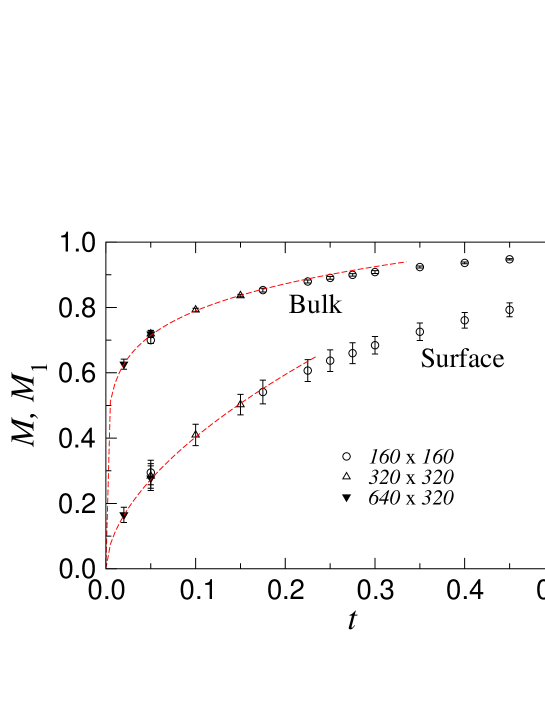
Figure 9: Temperature dependence of the bulk and boundary magnetisation ($q=8$, $r=10$, binary disorder).

The dots indicate the correction terms whose importance depend on the size of the system and on the distance from the transition temperature. Technically, one uses the definition of an effective temperature-dependent exponent, as illustrated in figures 9 and 10,

$$\beta_{\rm eff}(t)=\frac{{\rm d}\ln M(t)}{{\rm d}\ln t},\quad\beta=\lim_{t\to 0}\beta_{\rm eff}(t).$$

The precise value of the disorder strength $g$ of course also influences the value of $\beta_{\rm eff}(t)$ (playing a role in the corrections to scaling as mentioned above) but asymptotically the limit $t\to 0$ should be independent on $g$, since there is only one fixed point governing the disordered system.

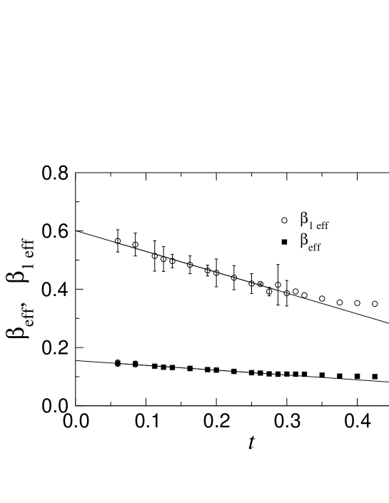
Figure 10: Temperature dependence of the exponents associated to the bulk and boundary magnetisation ($q=8$, $r=10$, binary disorder).

4.3 Finite-size scaling

One of the simplest method to extract critical exponents (once the critical temperature is known) is probably standard Finite-Size Scaling. On a finite system, the physical quantities cannot exhibit any singularity. They can be written as a singular term corrected by some scaling function which depends on the characteristic sizes of the problem, the correlation length $\xi$ and the size of the system $L$. In the case of the order parameter density for example we get $m_{L}(T)=|K-K_{c}|^{\beta}f(L/\xi)$. The function $f(x)$ of course depends on the geometry, but at the critical point $K_{c}$, the following behaviour is obtained:

$$M_{L}(K_{c})\mathop{\sim}_{L\to\infty}L^{-\beta/\nu}.$$ (35)

Here, the ratio $\beta/\nu$ is precisely the magnetic scaling dimension $x_{\sigma}$. An example is shown in figure 11 for the $8-$state Potts model. From the slopes of the curves, the values $\gamma/\nu=1.686(17)$, $\beta/\nu=0.152(4)$ and $\nu=1.005(30)$ can be obtained [64]. The results here are interesting as reference values that we shall compare with more sophisticated techniques later.

Figure 11: Finite-size scaling analysis of magnetisation, susceptibility and effective transition temperature shift for the critical self-dual binary disordered $8-$state Potts model.

4.4 Short-time dynamics scaling

It is commonly believed that universality can be found only in equilibrium stage of long-time regime in numerical simulations. For a magnetic system far from criticality, e.g. in the high temperature phase, suddenly quenched to the critical temperature, a universal dynamic scaling behaviour emerges already within the short-time regime, according to a simple generalisation of the homogeneity assumption for the order parameter [54, 55, 56, 59],

$$M(t,\tau,L,M_{0})=b^{-\beta/\nu}M(b^{1/\nu}t,b^{-z}\tau,b^{-1}L,b^{x_{0}}M_{0}),$$ (36)

where $z$ is the dynamic exponent (dependent on the choice of algorithm), $t=|K-K_{c}|$ is the deviation from the critical point, $M_{0}$ is the initial magnetisation with the associated scaling dimension $x_{0}$, and $\tau$ is the time (measured in MC sweeps). In the thermodynamic limit, $L\to\infty$, and at criticality, $t=0$, the expected evolution is given by $M(\tau,M_{0})=\tau^{-\beta/\nu z}f(M_{0}\tau^{-x_{0}/z})$ and allows the computation of the critical exponents. The main interest of short-time dynamics scaling is that it is not affected by critical slowing down, since only early time stages of the simulation are involved.

4.5 Conformal mappings

Monte Carlo simulations of two-dimensional spin systems are generally performed on systems of square shape while transfer matrix computations are done in strip geometries. In the following, we consider such a system of size $2N\times L$, and call $u$ and $v$ the corresponding directions (figure 12). The order parameter correlations between a point close to the surface, and a point in the bulk of the system should, in principle, lead to both surface and bulk critical exponents. Practically, it is not of great help for the accurate determination of critical exponents, since

i) strong surface effects (shape effects) occur which modify the large distance power-law behaviour,

ii) the universal scaling function entering the correlation function is likely to display a crossover before its asymptotic regime is reached (system-dependent effect).

                     

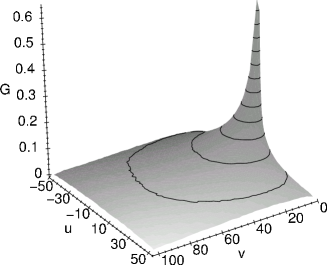
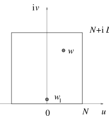
Figure 12: Monte Carlo simulations of the 2$d$ Ising model inside a square of $101\times 101$ lattice sites ($10^{6}$ MCS/spin, Swendsen-Wang cluster algorithm). The figure shows the correlation function between a point close to the surface ($w_{1}={i}$) and all other points $w$ in the square. The sketch on the right specifies the notations.

One can proceed as follows: systems of increasing sizes are successively considered, and the correlations are computed along $u$- (parallel to a square edge considered as the free surface) and $v$-axis (perpendicular to this edge). The order parameter correlation function for example is supposed to obey a scaling form which reproduces the expected power-law behaviour in the thermodynamic limit:

$$G_{\perp}(v)=\frac{1}{v^{x_{\sigma}+x_{\sigma}^{1}}}f_{\ \!{}_{sq.}}\left(\frac{v}{L}\right),\qquad G_{\parallel}(u)=\frac{1}{u^{2x_{\sigma}^{1}}}f^{\prime}_{\ \!{}_{sq.}}\left(\frac{u}{N}\right),$$ (37)

where $x_{\sigma}$ and $x_{\sigma}^{1}$ are, respectively, the bulk and surface order parameter scaling dimensions. The scaling functions $f_{\ \!{}_{sq.}}$ depends on the geometry, but have to satisfy asymptotic expansions including corrections to scaling e.g. $f_{\ \!{}_{sq.}}\left(\frac{v}{L}\right)\sim 1+{\rm const}\left(\frac{v}{L}\right)^{\epsilon}+\dots$ in the boundary region $v\to L$.

Figure 13: Monte Carlo simulations in the case of the two-dimensional Ising model. a) Log-log plot of the order parameter correlation function perpendicular to the surface ($v$-direction) and parallel to this surface ($u$-direction) for system sizes $101\times 101$ ($+$, $5.10^{6}$ MCS/spin) and $501\times 501$ ($\circ$, $2.10^{5}$ MCS/spin). The correlations are computed between a point $w_{1}={i}$ close to the surface and points $w={i}v$, and $w=u+{i}$ respectively. The corresponding estimations for $x_{\sigma}+x_{\sigma}^{1}$ and $2x_{\sigma}^{1}$ are written in the figure and the fit has been done in the range indicated by a dashed line. The figures correspond to power-law fits for the size $501^{2}$.b) Conformal rescaling of the perpendicular correlations for the two sizes (see below). The rescaled correlation function exhibits a true power-law in the whole range of variation of the new variable, and the value for $x_{\sigma}+x_{\sigma}^{1}$ is improved. The solid lines correspond to the theoretical asymptotic form while the dotted line is the exact expression in the continuum limit.

Equations (37) are not very useful for the determination of critical exponents, since at least five unknown quantities appear, and the correction terms in $f_{\ \!{}_{sq.}}(x)$ may have a large amplitude, resulting from the significance of finite-size corrections. Nevertheless, if the power-law fit is limited to the linear regions on a log-log scale (almost one decade in figure 13a), one gets correct estimations of the critical exponents, as long as condition ii) is fulfilled.

At a critical point, scale invariance coupled with rotation and translation invariance also implies covariance under local scale transformations, i.e. conformal transformations [6]. The conformal transformations are those general coordinate transformations which preserve the angle between any two vectors. They leave the metric invariant up to a scale change. The conformal group includes the Euclidean group as a subgroup, the dilatations and the special conformal transformations. In any dimension these conformal transformations are also called global conformal transformations because they map the infinite space onto itself. Consider a lattice model described in the continuum limit by a local theory defined by some action $S$. Conformal symmetry occurs when a local theory is scale invariant. In lattice systems, nearest–neighbour interactions ensure that physics is local and scale invariance holds at the critical point where a continuous limit description is allowed. For any local field (the energy density or the magnetisation for a spin system for example) the usual homogeneity assumption under a homogeneous rescaling ${\bf R}\to b{\bf R}$

$$\langle\phi(0)\phi(b{\bf R})\rangle=b^{-2x_{\phi}}\langle\phi(0)\phi({\bf R})\rangle$$ (38)

is extended to local transformations with a position dependent rescaling factor. In two dimensions conformal transformations are realized by the analytic functions in the complex plane (the conformal group is thus infinite-dimensional): $z\longrightarrow w(z)$ and equation (38) is thus generalised to a covariance law of transformation of the ($N-$point) correlators under conformal mappings:

$$\langle\phi(w_{1})\phi(w_{2})\rangle=\mid\!w^{\prime}(z_{1})\!\mid^{-x_{\phi}}\mid\!w^{\prime}(z_{2})\!\mid^{-x_{\phi}}\langle\phi(z_{1})\phi(z_{2})\rangle.$$ (39)

Here, $z_{1}$ and $z_{2}$ are two points in the original complex plane and $w_{1}$ and $w_{2}$ are the corresponding points in the transformed complex geometry under the mapping $w(z)$. This transformation law is very helpful in numerical analysis, since simulations or numerical computations are always performed on finite systems of particular shape, depending on the technique used. The critical properties of an infinite system $\langle\phi(z_{1})\phi(z_{2})\rangle\sim|z_{1}-z_{2}|^{-2x_{\phi}}$ can thus be obtained by fitting the numerical data to the transformed conformal expression which usually deviates significantly from a simple power law (although the algebraic decay at criticality must be recovered asymptotically in the limit of an infinite system of course). The situation is schematically sketched in figure 14

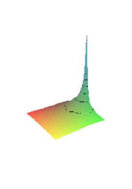
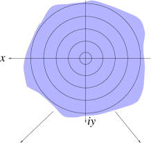
Figure 14: Conformal mapping of the infinite plane $z=x+iy$ inside a finite square $N\times N$ with free edges or a strip of width $L$ with periodic boundary conditions.

Among all the possible mappings, we shall here specify a few cases of interest:

i)

Mapping onto a cylinder: the logarithmic transformation

$$w(z)=\frac{L}{2\pi}\ln z=u+iv$$ (40)

is well known to map the infinite plane onto a strip of finite width $L$ with periodic boundary conditions and infinite length. This is the limit $N\to\infty$ in the rectangular geometry described above. Using the algebraic decay of the two-point correlator in the $z-$plane, one gets on the strip

$$\langle\phi(0,0)\phi(u,v)\rangle=\left(\frac{2\pi}{L}\right)^{2x_{\phi}}\left[2\cosh\left(\frac{2\pi u}{L}\right)-2\cos\left(\frac{2\pi v}{L}\right)\right]^{-x_{\phi}}.$$ (41)

In the long direction of the strip, at large distances it becomes an exponential decay

$$\langle\phi(0,0)\phi(u,0)\rangle_{\rm pbc}=\left(\frac{2\pi}{L}\right)^{2x_{\phi}}\exp\left({-\frac{2\pi ux_{\phi}}{L}}\right).$$ (42)

For sufficiently large strip widths, the transverse direction can also give some interesting results. Using the mapping $w(z)=\frac{L}{\pi}\ln z$, the half-infinite plane is mapped onto a strip with open boundaries in the transverse direction. If the boundary conditions are fixed (for example using an ordering surface field coupled to the order parameter) on one edge and free on the opposite edge (this is the meaning of the notation $+f$ below), the transverse profile of the order parameter density is given by the conformal expression

$$\langle\sigma(v)\rangle_{+f}={\rm const}\ \!\times\left[\frac{L}{\pi}\sin\left(\frac{\pi v}{L}\right)\right]^{-x_{\sigma}}F\left[\cos\left(\frac{\pi v}{2L}\right)\right].$$ (43)

The shape of the scaling function $F(x)$ is asymptotically constrained by simple scaling, $F(x)\sim x^{x_{\sigma}^{1}}$ (here, $x_{\sigma}^{1}$ is the boundary scaling dimension of the order parameter).

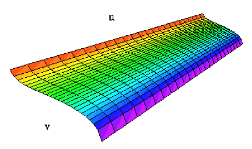
Figure 15: Transverse profiles of the order parameter in an infinitely long strip with fixed-free boundary conditions.

ii)

Mapping onto a square: the Schwarz-Christoffel transformation

$$w(z)={N\over 2{\rm K}}{\rm F}(z,k),\quad z={\rm sn}\left({2{\rm K}w\over N}\right)$$ (44)

maps the half-infinite plane $z=x+iy$ ($0\leq y<\infty$) inside a square $w=u+iv$ of size $N\times N$ ($-N/2\leq u\leq N/2$, $0\leq v\leq N$) with free boundary conditions along the four edges. Here, $F(z,k)$ is the elliptic integral of the first kind, ${\rm sn}\ \!(2{\rm K}w/N)$ the Jacobian elliptic sine, ${\rm K}=K(k)$ the complete elliptic integral of the first kind, and the modulus $k$ is solution of $K(k)/K(\sqrt{1-k^{2}})=\frac{1}{2}$.

In the semi-infinite geometry, the two-point correlator is fixed up to an unknown scaling function (apart from some asymptotic limits implied by scaling). Fixing one point $z_{1}$ close to the free surface ($z_{1}=i$) of the half-infinite plane, and leaving the second point exploring the rest of the geometry, $z_{2}=z$, the following behaviour is expected:

$$\langle\phi(z_{1})\phi(z)\rangle_{\frac{1}{2}\infty}\sim y^{-x_{\sigma}}\psi(\omega),$$ (45)

where the dependence on $\omega=\frac{y_{1}y}{\mid z_{1}-z\mid^{2}}$ of the universal scaling function $\psi$ is constrained by the special conformal transformation and its asymptotic behaviour, $\psi(\omega)\sim\omega^{x_{\phi}^{1}}$, in the limit $y\gg 1$, is implied by scaling.

Using the mapping (44), the local rescaling factor in equation (39) is obtained, $w^{\prime}(z)=\frac{N}{2{\rm K}}[(1-z^{2})(1-k^{2}z^{2})]^{-1/2}$, and inside the square the two-point correlation function becomes (see Ref. [44])

$$\langle\phi(w_{1})\phi(w)\rangle_{\rm sq.}\sim{\underbrace{\left(\Im[z].\left(|1-z^{2}|.|1-k^{2}z^{2}|\right)^{-1/2}\right)}_{\kappa(w)}}^{-x_{\phi}}\psi(\omega),$$ (46)

with $z(w)$ given by equation (44). This expression is correct up to a constant amplitude determined by $\kappa(w_{1})$ which is kept fixed, but the function $\psi(\omega)$ is still varying with the location of the second point, $w$.

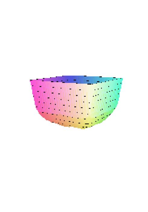
Figure 16: Profiles of the order parameter in a square with fixed boundary conditions.

In order to cancel the role of the unknown scaling function, it is more convenient to work with a density profile in the presence of ordering surface fields. This is a one-point correlator whose functional shape in the half-infinite geometry is determined by scaling apart from some amplitude:

$$\langle\sigma(z)\rangle_{\frac{1}{2}\infty}={\rm const\times}y^{-x_{\sigma}}$$ (47)

and it maps onto

$$\langle\sigma(w)\rangle_{\rm sq.}={\rm const\times}[\kappa(w)]^{-x_{\sigma}}$$ (48)

where the function $\kappa(w)$ again comes from the mapping.

The case of the mapping of the infinite complex plane inside a square with periodic boundary conditions was for example used in Ref. [73].

Other mappings can be convenient. Our choice here was motivated by the fact that Monte Carlo simulations are usually performed on samples of square shapes. On the other hand, the strip (with free or fixed boundary conditions) is the natural geometry generated in transfer matrix calculations.

4.6 Impact of rare events and non self-averaging

As we mentioned, the physical properties have to be averaged over many samples produced with a given probability distribution. One can typically encounter two opposite situations, depending on the quantities under interest. The average order parameter for example is defined as a sum of quantities affected by randomness,

$$\overline{\langle\sigma\rangle}=\frac{1}{N^{2}}\overline{\sum_{i}\langle\sigma_{i}\rangle}$$

while the correlation function

$$\langle\delta_{\sigma_{j}\sigma_{j+u}}\rangle\simeq\langle\Lambda_{0}\!\mid{\bf g}_{j}\left(\vphantom{\prod}\right.\prod_{k=j}^{j+u-1}{\bf T}^{\prime}_{k}\left.\vphantom{\prod}\right){\bf d}_{j+u}\mid\!\Lambda_{0}\rangle$$

essentially depends on a product of non-commuting matrices whose elements are determined by the disorder distribution. These two types of quantities definitely exhibit different properties as functions of the number of samples used to sample the probability distribution. When computing mean values, it is clear that the accuracy of the results for a given number of disorder realizations, does not have the same behaviour in the case of sums or of products of random variables. Consider as an example the sum and the product of random variables $\lambda_{i}$ taken from a binary distribution,

$$\Sigma_{\lambda}=\sum_{i=1}^{n}\lambda_{i},\quad\Pi_{\lambda}=\prod_{i=1}^{n}\lambda_{i},$$

and compute the moments (rescaled by a power $1/p$) $[\overline{(\Sigma_{\lambda})^{p}}]^{1/p}$ and $[\overline{(\Sigma_{\lambda})^{p}}]^{1/p}$ averaged over $N$ realizations of the $\lambda_{i}$’s (here we choose for this example $n=50$, so there are some $10^{15}$ configurations). Numerical results are given in the table 3 for some choice of parameters.

	$\Sigma_{\lambda}$				$\Pi_{\lambda}$
$N$	$p=1$	$p=5$	$p=20$	$p=50$	$p=1$	$p=5$	$p=20$	$p=50$
$10^{1}$	0.990	1.060	1.228	1.305	1.054	1.529	2.042	2.188
$10^{3}$	1.014	1.049	1.156	1.298	1.060	1.292	2.143	2.630
$10^{5}$	1.010	1.047	1.161	1.327	1.054	1.303	2.480	3.467
$10^{7}$	1.010	1.047	1.160	1.322	1.055	1.301	2.511	3.857

Table 3: Comparison between the moments of a sum and of a product of random variables distributed according to a bimodal probability distribution, as a function of the number of realizations.

It is particularly clear that the values obtained from the sum $\Sigma$ converge rapidly (the variations between results obtained at different number of realizations correspond to a statistical noise). This is due to the fact that $\Sigma$ is normally distributed, while in the case of the product $\Pi$, we note a continuous increase of the numerical estimate of a given moment as the number of samples increases and this effect is especially pronounced for high moment order $p$. This is due to the fact that the distribution of the $\Pi$’s is log-normal and thus there exist some events which have a dominant role in the average, but which are so rare that they are not scanned by a poor statistics which would essentially explore the region of typical values. In order to be more precise in the distinction between typical and average value, we rewrite $\ln\Pi$ as a sum of random variables, $\ln\Pi_{\lambda}=\sum_{i}\ln\lambda_{i}$, which, according to the central limit theorem, has a Gaussian distribution in the limit of large number of draws. The typical value corresponds to the maximum of the probability distribution, $\Pi_{\rm typ}={\rm e}^{\overline{\ln\Pi}}$ where the Gaussian is centered, and clearly differs from the average value $\overline{\Pi}=\overline{{\rm e}^{\ln\Pi}}$.

The same situation occurs when computing the spin-spin correlation function

$$\overline{\langle\sigma(0)\sigma(u)\rangle}_{\rm st}=\overline{G_{\sigma}(u)}.$$ (49)

Since it is almost log-normal (see figure 17), the logarithm of $G_{\sigma}(u)$ is self-averaging and the average $\overline{\ln G_{\sigma}(u)}$ as well as higher order moments are well behaved. A cumulant expansion is thus convenient to reconstruct the average $\overline{G_{\sigma}(u)}$ through

$$\overline{G_{\sigma}(u)}={\rm e}^{\overline{\ln G_{\sigma}(u)}+\frac{1}{2}(\overline{\ln^{2}G_{\sigma}(u)}-\overline{\ln G_{\sigma}(u)}^{2})+\dots}.$$ (50)

This is a test (see figure 17) which proves that the probability distribution is sufficiently well scanned with the large numbers of realizations used in this run.

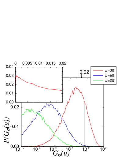
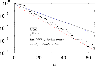
Figure 17: Top: Probability distribution of the spin-spin correlation function (8-state Potts model with bimodal disorder). The insert shows ${\cal P}(G_{\sigma}(u))$ (with a very long tail on the right), while it is shown on a logarithmic scale in the main frame, where one can notice the shape which is close to a log-normal distribution. Bottom: Reconstruction of the correlation function from the moments of its logarithm.

5 Numerical results and comparison with perturbative expansions in $2D$

5.1 Regime $q>4$

5.1.1 Randomness induces a second-order regime

Although there is no perturbation result for $q>4$, we shall start in the regime of first-order transition of the pure model. A first step was to prove that even for large numbers of states per spin, the transition was rounded to become continuous. That was done by different authors [39, 41]. Chen et al studied the free energy barrier $\Delta F(L)$, defined from the energy histogram ${\cal P}(E)$ in Monte Carlo simulations according to ${\rm e}^{-\beta\Delta F(L)}=P_{\rm max}/P_{\rm well}$, with $P_{\rm max}$ given by the maximum of ${\cal P}(E)$ and $P_{\rm well}$ corresponding to the value at the bottom of the well separating the two coexisting phases. They showed that the energy barrier $\Delta F(L)=-2\sigma_{\rm o.d.}L^{d-1}$ vanishes in the thermodynamic limit (figure 18)where $\sigma_{\rm o.d.}$ is the order-disorder interface tension between the two possibly coexisting phases.

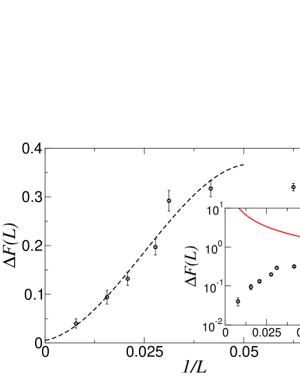
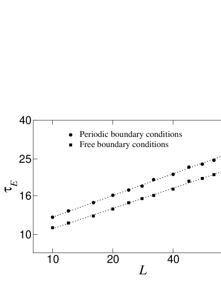
Figure 18: Top: Evolution of the free energy barrier with the size of the system for the $8-$state Potts model with binary disorder (at small disorder strength). The dotted line in the inset shows the case of the pure system (taken from Chen, Ferrenberg and Landau Ref. [39]). The dotted line is a guide for the eyes. Bottom: Power-law behaviour of the energy autocorrelation time in the $8-$state Potts model with binary disorder.

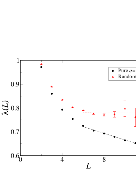
Figure 19: Evolution of the corrections to scaling to the free energy in a strip geometry (taken from Cardy and Jacobsen [41]).

The dynamics of the Monte Carlo simulations leads to compatible conclusions. The energy autocorrelation time $\tau_{E}$ is indeed exponentially large (with the system size) when a non vanishing order-disorder interface tension $\sigma_{\rm o.d.}$ exists,

$$\tau_{E}\sim L^{d/2}{\rm e}^{2\sigma_{\rm o.d.}L^{d-1}},$$

while it is only increasing as a power law at second-order transitions,

$$\tau_{E}\sim L^{z},$$

with a dynamical exponent $z$ which strongly depends on the algorithm used. This latter situation is indeed observed [64] in the disordered $8-$state Potts model (figure 18).

Cardy and Jacobsen on the other hand used transfer matrix calculations [41], measuring the free energy density $\bar{f}_{L}$ whose corrections to scaling behave at first-order transitions like $\bar{f}_{L}\sim l_{\infty}+O(L^{-d}{\rm e}^{-L/\xi})$. Plotting then $\lambda(L)=\ln(\bar{f}_{L}-f_{\infty})+d\ln L$ vs the strip width $L$ should give asymptotically a straight line with a slope given by the inverse correlation length $1/\xi$. In the presence of randomness, the curve corresponding to the $8-$state Potts model indicates a diverging correlation length as expected at a second-order phase transition (figure 19).

5.1.2 Comparison between finite-size scaling and conformal mappings

Conformal mappings provide quite efficient techniques for the determination of critical exponents. The validity of such an approach is nevertheless restricted to systems where scale invariance, translation invariance and rotation invariance do hold. This requirement is not obviously fulfilled in random systems, since disorder breaks the symmetries. Hopefully, one may expect that after averaging over many disorder realizations, one is led to some effective system for which these symmetries are restored. This assumption can be checked from numerical simulations. Studying the critical behaviour using an independent technique, namely finite-size-scaling which can safely be supposed to give the right results, we then compare to the exponents deduced from various mappings which are assumed to work. The comparison was performed carefully in the case of the $8-$state Potts model with binary disorder, and the technique was then applied in the regime $q>4$, and even to asymptotically large $q$’s [45]. The FSS results, which are considered here as the reference results, are shown in figure 11. In strip geometries, the correlation functions in the long direction and the order parameter profile in the transverse direction (figure 20) lead to compatible results.

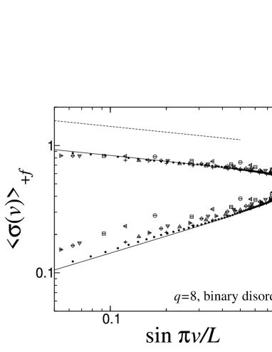
Figure 20: Fixed-free BC order parameter critical profile for the self-dual binary disordered $8-$state Potts model. The behaviour close to the fixed surface gives access to the bulk scaling dimension (the corresponding curve is shown in dotted line and the conformal expression is shown in full line while the symbols correspond to strips of various widths).

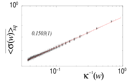
Figure 21: Fitting the correlation function (top) and the order parameter profile (bottom) in a square geometry. The different curves (top) correspond to different values of the variable $\omega$. This is the case $q=8$, with a binary distribution, at the optimal disorder strength estimated by the maximum of the central charge in strip geometry.

In the square geometry, the fit of the correlation function must be done along some curves inside the square where the scaling variable $\omega$ remains constant, which implies that the function $\psi(\omega)$ also remains constant and a simple power-law fit is then needed,

$$\overline{\langle\sigma(w_{1})\sigma(w)\rangle}_{\rm sq}\sim A_{\omega}|\kappa(w)|^{-x_{\sigma}},$$

where $A_{\omega}$ stands for the amplitude which contains $\psi(\omega)$ ($w_{1}$ is fixed and chosen equal to imaginary unit $w_{1}={i}$). A difficulty occurs due to discretization of the lattice Estimation of the correlation function along the continuous curve $\omega={\rm const.}$ is done using a Taylor expansion from the data taken at 4 neighbour points on each plaquette. This explains the non monotonic behaviour of the error bars in figure 21.

The case of the density profile is better to achieve, since it involves no unknown scaling function, but a single constant amplitude (it is a one-point correlator). All the points inside the square enter the power-law fit

$$\overline{\langle\sigma(w)\rangle}_{\rm sq}\sim{\rm const}\times|\kappa(w)|^{-x_{\sigma}}$$

and make it more accurate (and there is no need of any expansion around the lattice points). The number of points ($N^{2}$) being so large, we can even forget uncertainties on each point and simply take as error bar on the resulting exponent the standard deviation.

$x^{\prime}_{\sigma}$ for the $8-$state Potts model with binary disorder
Technique	Quantity	Scaling dimension	Ref.
Standard techniques
$t-$dependence	$\overline{M_{b}(t)}$	0.151(1)	[33]
FSS	$\overline{M_{b}(K_{c})}$	0.153(1)	[28, 29]
FSS	$\overline{\langle\sigma(0)\sigma(L/2)\rangle}$	0.159(3)	[34]
Short-time dynamics	$\overline{M_{b}(\tau)}$	0.151(3)	[54]
Conformal mappings
Periodic strip	$\overline{\langle\sigma(0)\sigma(u)\rangle}_{\rm st}$	0.1505(3)	[30, 44, 64]
Free BC square	$\overline{\langle\sigma(0)\sigma(w)\rangle}_{\rm sq}$	0.152(3)	[30, 44, 64]
Fixed-free strip	$\overline{\langle\sigma(v)\rangle}_{\rm st}$	0.150(1)	[33, 64]
Fixed BC square	$\overline{\langle\sigma(w)\rangle}_{\rm sq}$	0.1503(1)	[30, 44, 64]

Table 4: Comparison between temperature-dependence, FSS and short-time dynamics scaling results for the magnetic exponent $\beta^{\prime}/\nu^{\prime}$ and the scaling dimension $x^{\prime}_{\sigma}$ at the random fixed point deduced from the logarithmic and the Schwarz-Christoffel mappings for the $8-$state Potts. In the first line, the exponent $\beta^{\prime}$ deduced from the temperature dependence is close to $x^{\prime}_{\sigma}$, since the value of the correlation length exponent is found very close to 1 ($\nu^{\prime}\simeq 1.01(1)$). We note also that in all these references but Ref. [34], a binary distribution of disorder was used.

The results for the magnetic scaling dimension measured using Finite-Size Scaling techniques, compared to the mappings onto strips or square geometries, are compared in table 4 in the case of the $8-$state Potts model with a self-dual binary probability distribution of coupling strengths. First we note that the transition is second-order, even in the regime $q>4$, as predicted by the Imry-Wortis agreement. More important for the following is the fact that the agreement between different techniques is quite fair and leads to the conclusion that conformal techniques can be applied here, in spite of the lack of the symmetry properties which should in principle be required. This is due to the fact that we are interested in average quantities. The system thus becomes, on average, translationnaly, rotationally invariant, as well as scale invariant at the critical point. This is an important point, because the use of conformal mappings is more accurate than standard FSS methods, and the comparison between different schemes in the $2\leq q\leq 4$ regime will require a great accuracy, as already noticed in table 2.

5.2 Regime $q\leq 4$

5.2.1 Tests of replica symmetry

First of all, the fitting procedure has to be validated. From the exponential decay of the average spin-spin correlation function, the exponent $x^{\prime}_{\sigma}$ is deduced and presented as a function of $q$ for the case of a binary disorder in Fig. 22. These results were first reported by Cardy and Jacobsen in Ref. [41]. The agreement with the third order expansion in equation (20) is extremely good especially in the region where the expansion is supposed to be valid when $q$ is not too far from the Ising model value $q=2$. The quality of the data confirms the reliability of the averaging procedure (table 5). Even close to the marginally irrelevant case of the Ising model where logarithmic corrections are known to be present for some quantities, we note that the numerical data are quite satisfactorily in agreement with the perturbative results. The agreement is made better by the absence of logarithmic corrections for the average correlation function at $q=2$, and we will see that this observation is no longer true in the following study of other moments.

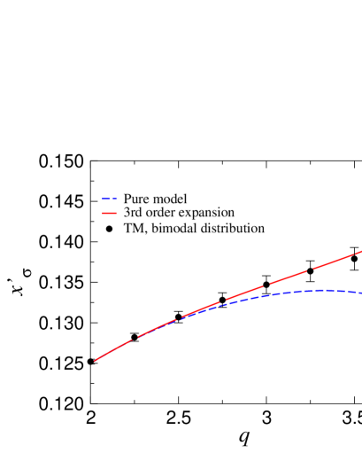
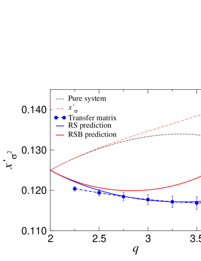
Figure 22: Top: Scaling dimension of the order parameter (binary disorder) compared to the third order expansion of Dotsenko and co-workers [20]. The scaling dimension corresponding to the pure model is shown for comparison. Bottom: Exponent of the second moment of the spin-spin correlation function as a function of the number of states of the disordered Potts model (binary disorder). The comparison is done with Replica Symmetry and Replica Symmetry Breaking scenarios [25]. The agreement with the RS result is quite good around $q=3$. When $q$ is close to 2, the discrepancy can be attributed to the weak relevance of disorder. We indeed used a simple exponential fit as can be expected at a stable disordered FP, but at $q=2$, one knows from Ludwig’s results that logarithmic corrections must be added. These corrections can also influence the vicinity of $q=2$ in a numerical approach.

The question of a possible breaking of replica symmetry in disordered systems is very controversial and far from being settled, especially in spin glasses (see e.g Refs. [103, 104, 105, 106, 107]). In the context of disordered Potts ferromagnets, the question was first addressed by Dotsenko et al [25]. In order to test between Replica Symmetry and Replica Symmetry Breaking schemes, Dotsenko et al performed a second order expansion of the exponent of the second moment of the spin-spin correlation function decay in both cases (Equations (24)). MC simulations were first performed at $q=3$ but were not completely conclusive, although in favour of Replica Symmetry: the perturbation expansion leads to $x^{\prime}_{\sigma^{2}}(3)=0.1176$ and $x^{\prime\prime}_{\sigma^{2}}(3)=0.1201$ according to equations (24), while previous numerical results lead to $0.113(1)$ [25], $0.1140(5)$ [63], $0.116(1)$ [33] and $0.119(2)$ [34].

$q$	$x^{\prime}_{\sigma}$
	Expansion (20)	TM result (Ref. [46])
2	0.12500	0.1252(3)
2.25	0.12800	0.1282(5)
2.5	0.13051	0.1307(7)
2.75	0.13269	0.1328(9)
3.	0.13465	0.1347(11)
3.25	0.13653	0.1364(13)
3.5	0.13845	0.1379(14)

Table 5: Comparison of the numerical results for the magnetic scaling dimension (bimodal probability distribution) $x^{\prime}_{\sigma}$ with the third order expansion of Dotsenko and co-workers [20]. The error bars systematically contain the analytical value.

$q$	Perturbative results		TM result
	$x^{\prime}_{\sigma^{2}}$	$x^{\prime\prime}_{\sigma^{2}}$	(Ref. [46])
2.25	0.12213	0.12229	0.1204(5)
2.5	0.12002	0.12067	0.1194(8)
2.75	0.11854	0.11997	0.1185(10)
3.	0.11761	0.12011	0.1177(12)
3.25	0.11718	0.12110	0.1172(14)
3.5	0.11723	0.12304	0.1169(16)
	$x^{\prime}_{\varepsilon}$	$x^{\prime\prime}_{\varepsilon}$	(Ref. [47])
2.5	1.006	1.000	1.00(1)
2.75	1.013	1.000	1.01(1)
2.5	1.023	1.000	1.02(1)

Table 6: Decay exponent of the second moment of the spin-spin correlation function compared to Replica Symmetry and Replica Symmetry Breaking expressions of Eqs. (24). The results written in bold face correspond to the range of values of $q$ where the agreement is particularly satisfactory. The second part of the table presents Jacobsen’s results [47] for the exponent of the average energy correlation function.

Conclusive results for different values of $q$ were then obtained using transfer matrices. Close to $q=2$, the proximity of the marginally irrelevant Ising FP will surely alter the data, as a reminiscent effect of the logarithmic corrections present exactly at $q=2$ for the second moment [17, 108]. Too large values of $q$ on the other hand are not very helpful in order to check perturbation expansions which break down when one explores higher values of the expansion parameter. One thus has to balance between these two extreme situations and the comparison between numerical data and perturbation results should be conclusive around $q=3$ or slightly below. The TM technique thus appears to be well adapted, since it is capable to deal with non integer values of $q$. The comparison is shown in Fig. 22 for the bimodal probability distribution and the results are also given in table 6. In the convenient domain for the test, around $q=3$, results are written in bold face. The agreement with Replica Symmetry is quite convincing. The results for the exponent associated to the average energy-density correlations [47] confirm this conclusion.

5.2.2 Multiscaling

The multiscaling behaviour of the spin-spin correlation functions is noticeable in the $p-$dependent set of exponents of the reduced moments

$$\overline{\langle\sigma(0)\sigma(R)\rangle^{p}}^{1/p}.$$

In Ref. [46], exhaustive computation of 50 different moments in the range $0\leq p\leq 5$ were performed in the strip geometry, and the associated scaling dimensions followed from a semi-log fit $\ln\overline{\langle\sigma(0)\sigma(u)\rangle^{p}}$ vs $\ln u$, followed by an extrapolation to $L\to\infty$. The numerical results were compared to the first order expansion of Ludwig and to the second order expansion in the RS scheme in Eq. (26). The second order result is clearly very good up to values of $p$ close to 3 and then breaks down as already noticed by Lewis [63].

An alternate presentation of the results (used e.g. by Ludwig [19]) is given by the scaling dimension of the moment of the correlation function itself, $\overline{\langle\sigma(0)\sigma(R)\rangle^{p}}$ (not the reduced function $\overline{\langle\sigma(0)\sigma(R)\rangle^{p}}^{1/p}$). The scaling dimension is thus simply $px^{\prime}_{\sigma^{p}}(q)$, hereafter denoted by $X^{\prime}_{\sigma^{p}}(q)$. An example, with $q=3$, is shown in Fig. 23 where we have shown the results obtained with the bimodal and the continuous self-dual probability distributions at the optimal disorder amplitude as well as the dilution case at optimal dilution. Once again, we find a fair agreement between the numerical data and the perturbative result which confirms universality, i.e. the exponent associated to a given moment of the correlation function does not depend on the detailed probability distribution of the coupling strengths.

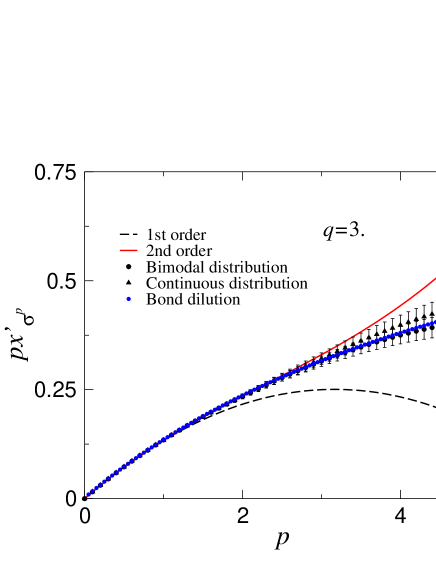
Figure 23: Comparison of the multi-fractal exponents (moment of the correlation function $\overline{\langle\sigma(0)\sigma(u)\rangle^{p}}$) with the second order expansion of Lewis in the RS scheme [26] for both the bimodal and the continuous probability distributions.

	average		typical
$q$	$x^{\prime}_{\varepsilon^{1}}$	TM	$x^{\prime}_{\varepsilon^{0}}$	TM
2.5	1.006	1.00(1)	1.023	1.02(1)
2.75	1.013	1.01(1)	1.051	1.04(2)
3.	1.023	1.02(1)	1.090	1.06(3)

Table 7: Decay exponent of the average and typical energy-energy correlation functions: comparison between perturbative expansion from Ref. [27] and transfer matrix computation (from Jacobsen [47]).

5.2.3 Probability distribution of correlation functions

In Ref. [19], Ludwig presented a remarquable discussion of the spin-spin correlation function probability distribution. The relevant information on the large distance behaviour is encoded in the multiscaling function $H(\alpha)$, which is simply the Legendre transform of the set of independent scaling indexes $X^{\prime}_{\sigma^{p}}(q)$. Setting ${\rm d}X^{\prime}_{\sigma^{p}}(q)=\alpha{\rm d}p$, this function is simply obtained by

$$H(\alpha)=X^{\prime}_{\sigma^{p}}(q)-\alpha p.$$

The geometrical interpretation of this Legendre transform follows from the relation $\frac{\partial H}{\partial\alpha}=-p$ where $\alpha$ is defined by $\frac{\partial X^{\prime}_{\sigma^{p}}(q)}{\partial p}=\alpha$. The scaling dimension $x^{\prime}_{\sigma^{p}}(q)$ is obtained on the plot of $H(\alpha)$ by the intercept of the tangent of slope $-p$ with the abscissa axis. An example of multiscaling function $H(\alpha)$ deduced from the numerical data with the bimodal probability distribution is shown in Fig. 24.

In this section, we follow Ludwig’s arguments and report a numerical study of the correlation function probability distribution in the cylinder geometry.

According to the results of the previous section, the moments of the spin-spin correlation function along the strip asymptotically behaves as follows:

$$\overline{G^{p}(u)}\equiv\overline{\langle\sigma(0)\sigma(u)\rangle^{p}}\sim B_{p}{\rm e}^{-\frac{2\pi u}{L}X^{\prime}_{\sigma^{p}}}$$ (51)

and are defined in terms of the probability distribution ${\cal P}[G(u)]$:

$$\overline{G^{p}(u)}=\int_{0}^{1}{\rm d}G(u){\cal P}[G(u)]G^{p}(u).$$ (52)

Following Ludwig, we introduce the variable $Y(u)=-\ln G(u)$ and write $G^{p}(u)={\rm e}^{-pY(u)}$. Using the identity ${\cal P}[G(u)]{\rm d}G={\cal P}[Y(u)]{\rm d}Y$ and equations (51) and (52), one obtains

$$\int_{0}^{\infty}{\rm d}Y(u){\cal P}[Y(u)]{\rm e}^{-pY(u)}\sim B_{p}{\rm e}^{-\frac{2\pi u}{L}X^{\prime}_{\sigma^{p}}}$$

which leads to the expression of the probability distribution by inverting the Laplace transform ($\delta>0$):

$${\cal P}[Y(u)]=\frac{1}{2{i}\pi}\lim_{\delta\to 0}\int_{\delta-{i}\infty}^{\delta+{i}\infty}{\rm d}pB_{p}{\rm e}^{-\frac{2\pi u}{L}\left[X^{\prime}_{\sigma^{p}}-\frac{Y(u)}{2\pi u/L}p\right]}.$$

The amplitude $B_{p}$ is assumed to be smoothly dependent on $p$ (this can be checked numerically), and its dependence can be forgotten with respect to the exponential, since it only introduces a correction when $2\pi u/L\to\infty$. Let us define the function $h(p)=X^{\prime}_{\sigma^{p}}-\frac{Y(u)}{2\pi u/L}p$. In the large distance limit $2\pi u/L\to\infty$, the integral can be evaluated by the saddle-point approximation at the minimum $p_{0}$ of $h(p)$:

$$\left(\frac{\partial}{\partial p}X^{\prime}_{\sigma^{p}}\right)_{p_{0}}=\frac{Y(u)}{2\pi u/L}$$

Instead of $Y(u)$, we define the scaled variable $\alpha=\frac{Y(u)}{2\pi u/L}$, and the saddle point value at $p_{0}$ only depends on this variable $h(p_{0})=H(\alpha)$. We thus obtain the probability distribution

$${\cal P}[Y(u)]\sim\exp\left[{-\frac{2\pi u}{L}H\left(\frac{Y(u)}{2\pi u/L}\right)}\right],$$ (53)

or, using ${\cal P}[Y(u)]{\rm d}Y={\cal P}(\alpha){\rm d}\alpha$,

$${\cal P}(\alpha)\sim\frac{2\pi u}{L}\exp\left[{-\frac{2\pi u}{L}H(\alpha)}\right].$$ (54)

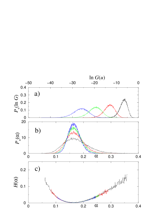
Figure 24: Fitting the probability distribution of the spin-spin correlation function to get a collapse onto a universal multiscaling function.

The multi-fractal function contains the essential information on the probability distribution. A correction to the leading behaviour given by the saddle-point approximation is needed here to improve the data collapse onto a single multiscaling function. If we expand the function $h(p)$ close to $p_{0}$, $h(p)\simeq H(\alpha)+\frac{1}{2}h^{\prime\prime}(p_{0})(p-p_{0})^{2}$, with $h^{\prime\prime}(p_{0})>0$ we obtain, instead of Eq. (53), the following result for the probability distribution ${\cal P}[Y(u)]$ [109]:

$${\cal P}[Y(u)]\sim\left(\frac{2\pi u}{L}\right)^{-1/2}\exp\left[{-\frac{2\pi u}{L}H\left(\frac{Y(u)}{2\pi u/L}\right)}\right]$$ (55)

and a correction appears in ${\cal P}(\alpha)$:

$${\cal P}(\alpha)\sim\left(\frac{2\pi u}{L}\right)^{1/2}\exp\left[{-\frac{2\pi u}{L}H(\alpha)}\right].$$ (56)

which enables to extract $H(\alpha)$ at fixed $\alpha$ by fitting the probability distribution to the expression

$$\ln{\cal P}(\alpha)-\frac{1}{2}\ln\frac{2\pi u}{L}={\rm const}-\frac{2\pi u}{L}H(\alpha).$$ (57)

It is shown in Fig. 24 where the probability distribution of the spin-spin correlation function was obtained after collecting the results over $96\ 000$ disorder realizations in 50 classes [46]. All the data collapse onto a single multiscaling function $H(\alpha)$, for different distances $u$ and this is even the case with still good accuracy for different strip widths or different probability distributions [46, 48].

6 Conclusion and summary of the main results

The two-dimensional Potts model is the ideal framework to test the influence of quenched randomness on phase transitions and critical behaviour. It exhibits a second-order phase transition completely characterised by conformal invariance when the number of states per spin is lower or equal to 4 and a first-order transition above. The transition line is exactly known, and it is easy to build in the random case probability distributions of coupling strengths which preserve the self-duality relation.

With respect to these advantages, many results concerning the effect of a weak disorder were obtained during the last decade using perturbations expansions around the pure fixed point. Different solutions were considered, first replica symmetric solutions where the symmetry between all the replicas is supposed to be preserved in the renormalization equations, then the case of a spontaneous breaking of the replica symmetry was also studied perturbatively.

Numerical studies were also performed from different sides. First of all, Monte Carlo simulations coupled to finite-size scaling analysis, then transfer matrices and sophisticated graph and loop algorithms coupled to extensive use of conformal mappings in order to extract the values of the critical exponents with a pretty good accuracy. All the results were in a fair agreement with the perturbative expansions close to the Ising model limit and concluded in favour of replica symmetric scenarios. The multiscaling properties of the order-parameter and energy density were also analysed, and a characterisation of the probability distributions of the correlation functions was made in terms of universal multiscaling functions. The regime $q>4$ where the pure model exhibits a first order transition was also extensively studied, but did not display any particular features compared to the regime $q\leq 4$ in the presence quenched randomness.

The most important question which remains open up to now is the identification of the conformal field theories which could describe the random fixed point. This is a delicate program, since in the replica limit of coupled models, the theory is not unitary (with a central charge which evolves continuously with the value of $q$). We may hope some progress in this direction for the near future, which would undoubtedly achieve a considerable progress in the understanding of two-dimensional disordered systems.

Acknowledgement

The material discussed here was partly presented at the Helsinki SPHINX ESF Conference 2002 on Disordered systems at low temperatures and their topological properties, and at the Ising lectures 2002 at Lviv. BB greatly acknowledges the organisers of the Helsinki workshop, M. Alava and H. Rieger and of the Lviv lectures, Y. Holovatch, I. Mryglod, and K. Tabunshchyk, for the opportunity given to present this review.

References

- [1] A.B. Harris, J. Phys. C 7, 1671 (1974).
- [2] Y. Imry and M. Wortis, Phys. Rev. B 19, 3580 (1979).
- [3] M. Aizenman and J. Wehr, Phys. Rev. Lett. 62, 2503 (1989).
- [4] K. Hui and A.N. Berker, Phys. Rev. Lett. 62, 2507 (1989).
- [5] S.K. Ma, Modern theory of critical phenomena, Benjamin Inc., Reading 1976.
- [6] J.L. Cardy,Scaling and renormalization in statistical physics, Cambridge University Press, Cambridge 1996.
- [7] Vik. Dotsenko, Introduction to the replica theory of disordered statistical systems, Cambridge University Press, Cambridge 2001.
- [8] R.B. Stinchcombe (1983), In Phase Transitions and Critical Phenomena vol. 7, C. Domb and J.L. Lebowitz eds. (London: Academic Press), p. 152.
- [9] A. Aharony, Phys. Rev. B 18, 3318 (1978).
- [10] Y. Imry and S.K. Ma, Phys. Rev. Lett 35, 1399 (1975).
- [11] G. Grinstein and S.K. Ma, Phys. Rev. Lett 49, 684 (1982).
- [12] J. Bricmont and A. Kupiainen, Phys. Rev. Lett 59, 1829 (1987).
- [13] Y.S. Shapir and A. Aharony, J. Phys. C 14, L905 (1981).
- [14] A. Aharony, Phys. Rev. B 12, 1038 (1975).
- [15] M. Dudka, R. Folk and Yu. Holovatch, 4 77, 2001 (Cond. Matt. Phys.).
- [16] F.Y. Wu, Rev. Mod. Phys. 54, 235 (1982).
- [17] A.W.W. Ludwig, Nucl. Phys. B 285 [FS19], 97 (1987).
- [18] A.W.W. Ludwig and J.L. Cardy, Nucl. Phys. B 330 [FS19], 687 (1987).
- [19] A.W.W. Ludwig, Nucl. Phys. B 330, 639 (1990).
- [20] Vl. Dotsenko, M. Picco and P. Pujol, Nucl. Phys. B 455 [FS], 701 (1995), hep-th/9501017.
- [21] Vl. Dotsenko, M. Picco and P. Pujol, Phys. Lett. B 347, 113 (1995), hep-th/9405003.
- [22] Vik. Dotsenko, Vl. Dotsenko, M. Picco and P. Pujol, Europhys. Lett. 32, 425 (1995), hep-th/9502134.
- [23] Vl. Dotsenko, M. Picco and P. Pujol, Nucl. Phys. B, Proceedings-Supplements 45 A, 145 (1996), cond-mat/9509149.
- [24] G. Jug and B.N. Shalaev, Phys. Rev. B 54, 3442 (1996).
- [25] Vik. Dotsenko, Vl. Dotsenko and M. Picco, Nucl. Phys. B250, 633 (1998), hep-th/9709136.
- [26] M.A. Lewis, Europhys. Lett. 43, 189 (1998), Erratum, Europhys. Lett. 47, 129 (1999), cond-mat/9710312.
- [27] M. Jeng and A.W.W. Ludwig, Nucl. Phys. B594, 685 (2001), cond-mat/9910181.
- [28] M. Picco, e-print cond-mat/9802092.
- [29] C. Chatelain and B. Berche, Phys. Rev. Lett 80, 1670 (1998), cond-mat/9801028.
- [30] C. Chatelain and B. Berche, Phys. Rev. E 58, R6899 (1998), cond-mat/9810270.
- [31] F. Yaa̧sar, Y. Gündüç and T. Çelik, Phys. Rev. E 58, 4210 (1998).
- [32] B. Berche and C. Chatelain, Comp. Phys. Comm. 121-122, 191 (1999).
- [33] G. Palágyi, C. Chatelain, B. Berche and F. Iglói, Eur. Phys. J. B 13, 357 (2000), cond-mat/9906067.
- [34] T. Olson and A.P. Young, Phys. Rev. B 60, 3428 (1999), cond-mat/9903068.
- [35] R. Paredes and J. Valbuena, Phys. Rev. E 59, 6275 (1999).
- [36] S. Wiseman and E. Domany, Phys. Rev. E 51, 3074 (1995), cond-mat/9411046.
- [37] J.K. Kim, Phys. Rev. B 53, 3388 (1996), cond-mat/9506117.
- [38] S. Chen, A.M. Ferrenberg and D.P. Landau, Phys. Rev. Lett. 69, 1213 (1992).
- [39] S. Chen, A.M. Ferrenberg and D.P. Landau, Phys. Rev. E 52, 1377 (1995).
- [40] U. Glaus, J. Phys. A 20, L595 (1987).
- [41] J.L. Cardy and J.L. Jacobsen, Phys. Rev. Lett. 79, 4063 (1997), cond-mat/9705038.
- [42] M. Picco, Phys. Rev. Lett. 79, 2998 (1997).
- [43] J.L. Jacobsen and J.L. Cardy, Nucl. Phys. B 515, 701 (1998), cond-mat/9711279.
- [44] C. Chatelain and B. Berche, Phys. Rev. E 60, 3853 (1999), cond-mat/9902212.
- [45] J.L. Jacobsen and M. Picco, Phys. Rev. E 61, R13 (2000), cond-mat/9910071.
- [46] C. Chatelain and B. Berche, Nucl. Phys. B 572, 626 (2000), cond-mat/9911221.
- [47] J.L.L. Jacobsen, Phys. Rev. E 61, R6060 (2000), cond-mat/9912304.
- [48] C. Chatelain, B. Berche and L.N. Shchur, J. Phys. A 34, 9593 (2001), cond-mat/0108014.
- [49] A. Roder, J. Adler, and W. Janke, Phys. Rev. Lett 80, 4697 (1998).
- [50] A. Roder, J. Adler, and W. Janke, Physica A 265, 28 (1999).
- [51] M. Hellmund and W. Janke, Nucl. Phys. B (Proc. Suppl.) 106, 923 (2002).
- [52] M. Hellmund and W. Janke, e-print cond-mat/0206400.
- [53] W. Janke, private communication.
- [54] H.P. Ying and K. Harada, Phys. Rev. E 62, 174 (2000), arXiv: cond-mat/0001284.
- [55] Z.Q. Pan, H.P. Ying and D.W. Gu, arXiv: cond-mat/0103130.
- [56] H.P. Ying, B.J. Bian, D.R. Ji, H.J. Luo and L. Schuelke arXiv: cond-mat/0103355.
- [57] H.P. Ying, Z.Q. Pan, H.J. Luo, S. Marculsecu and L. Schülke, Nucl. Phys. (Proc. Suppl.) 106, 920 (2002).
- [58] H.P. Ying, H. Ren, H.J. Luo and L. Schülke, Phys. Lett. A 298, 60 (2002).
- [59] C. Deroulers and A.P. Young, arXiv: cond-mat/0202135.
- [60] R. Juhasz, H. Rieger and F. Iglói, Phys. Rev. E 64, 056122 (2001), cond-mat/0106217.
- [61] P. Pujol, Théories conformes et systèmes désordonnés, Ph.D. dissertation, Université Pierre et Marie Curie, Paris VI, 1996, http://thesesENligne.ccsd.cnrs.fr/.
- [62] J.L. Jacobsen, Frustration and disorder in discrete lattice models, Ph.D. dissertation , Åarhus University 1998, http://ipnweb.in2p3.fr/ lptms/membres/jacobsen.
- [63] M.-A Lewis, Théorie des champs conformes: Systèmes désordonnés, couplés et modèle d’Ising sur variétés à bords, Ph.D. dissertation, Université Pierre et Marie Curie, Paris VI, 1999.
- [64] C. Chatelain, Influence du désordre sur les propriétés critiques du modèle de Potts, Ph.D. dissertation , Université Henri Poincaré, Nancy 1, 2000, http://thesesENligne.ccsd.cnrs.fr/.
- [65] T. Davis, Effects of quenched disorder on the behaviour of low-dimensional systems, Ph.D. dissertation, Oxford University, 2001.
- [66] Vik.S. Dotsenko and Vl.S. Dotsenko, Adv. Phys. 32, 129 (1983).
- [67] B.N. Shalaev, Phys. Rep. 237, 129 (1994).
- [68] W. Selke, L.N. Shchur and A.L. Talapov (1994), In Annual Reviews of Computational Physics vol 1, D. Stauffer ed. (Singapore: World Scientific), p. 17
- [69] J.S. Wang, W. Selke, Vl.S. Dotsenko and V.B. Andreichenko, Physica A 164, 221 (1990).
- [70] J.S. Wang, W. Selke, Vl.S. Dotsenko and V.B. Andreichenko, Europhys. Lett. 11, 301 (1990).
- [71] V.B. Andreichenko, Vl.S. Dotsenko, W. Selke and J.S. Wang, Nucl. Phys. B344, 531 (1990).
- [72] A.L. Talapov and L.N. Shchur, Europhys. Lett. 27, 193 (1994).
- [73] A.L. Talapov and Vl.S. Dotsenko, e-print cond-mat/9306027.
- [74] B. Derrida, Phys. Rep. 103, 29 (1984).
- [75] A. Aharony and A.B. Harris, Phys. Rev. Lett 77, 3700 (1996).
- [76] S. Wiseman and E. Domany, Phys. Rev. Lett 81, 22 (1998).
- [77] S. Wiseman and E. Domany, Phys. Rev. E 58, 2938 (1998).
- [78] Ch. V. Mohan, H. Kronmüller and M. Kelsch, Phys. Rev. B 57, 2701 (1998).
- [79] L. Schwenger, K. Budde, C. Voges and H. Pfnür, Phys. Rev. Lett 73, 296 (1994).
- [80] E. Domany, M. Schick, J.S. Walker and R.B. Griffiths, Phys. Rev. B 18, 2209 (1978).
- [81] C. Rottman, Phys. Rev. B 24, 14821 (1981).
- [82] M. Sokolowski and H. Pfnür, Phys. Rev. B 49, 7716 (1994).
- [83] K. Budde, L. Schwenger, C. Voges, and H. Pfnür, Phys. Rev. B 52, 9275 (1995).
- [84] C. Voges and H. Pfnür, Phys. Rev. B 57, 3345 (1998).
- [85] J.L. Cardy, M. Nauenberg and D.J. Scalapino, Phys. Rev. B 22, 2560 (1980).
- [86] M.E. Fisher, Phys. Rev. 176, 257 (1968).
- [87] D. Friedan, Z. Qiu and S. Shenker, Phys. Rev. Lett 52, 1575 (1984).
- [88] A.Z. Patashinskii and V.L. Prokowskii, Fluctuation theory of phase transitions, Pergamon Press, Oxford 1979.
- [89] A.M. Polyakov, Sov. Phys. JETP 36, 12 (1973).
- [90] W. Janke, in Computational Physics: Selected Methods - Simple Exercises - Serious Applications, edited by K.H. Hoffmann and M. Schreiber (Springer, Berlin, 1996).
- [91] G.T. Barkema and M.E.J. Newmann, in Monte Carlo Methods in Chemical Physics, Advances in Chemical Physics 105 edited by D. Ferguson, J. I. Siepmann, and D. G. Truhlar (Wiley, New York, 1999).
- [92] P.W. Kasteleyn and C.M. Fortuin, J. Phys. Soc. Japan 26 Suppl., 11 (1969).
- [93] R.H. Swendsen and J.S. Wang, Phys. Rev. Lett. 58, 86 (1987).
- [94] U. Wolff, Phys. Rev. Lett 62, 361 (1989).
- [95] H.W.J. Blöte and M.P. Nightingale, Physica (Amsterdam) 112A, 405 (1982).
- [96] V. Dotsenko, J.L. Jacobsen, M.-A. Lewis and M. Picco, Nucl. Phys. B 546, 507 (1999).
- [97] H. Furstenberg, Trans. Am. Math. Soc. 108, 377 (1963).
- [98] A.B. Zamolodchikov, JETP Lett. 43, 730 (1986).
- [99] L. Chayes and K. Shtengel, e-print cond-mat/981103.
- [100] L. Turban, Phys. Lett. 75A, 307 (1980).
- [101] L. Turban, J. Phys. C 13, L13 (1980).
- [102] P. Guilmin and L. Turban, J. Phys. C 13, 4077 (1980).
- [103] M. Mézard, G. Parisi and M.A. Virasoro, Spin Glass Theory and beyond, World Scientific (Singapore, 1987).
- [104] E. Marinari, G. Parisi, J. Ruiz-Lorenzo and F. Ritort, Phys. Rev. Lett. 76, 843 (1996).
- [105] E. Marinari, C. Naitza, F. Zuliani, G. Parisi, M. Picco and F. Ritort, Phys. Rev. Lett. 81, 1698 (1999).
- [106] H. Bokil, A.J. Bray, B. Drossel and M.A. Moore, Phys. Rev. Lett. 82, 5174 (1999).
- [107] E. Marinari, C. Naitza, F. Zuliani, G. Parisi, M. Picco and F. Ritort, Phys. Rev. Lett. 82, 5175 (1999).
- [108] S.L.A. de Queiroz and R.B. Stinchcombe, Phys. Rev. E 54, 190 (1996), cond-mat/9604053.
- [109] N.G. De Bruijn, Asymptotic methods in analysis, Dover, New-York, 1981.
- [110] B. Fourcade and A.-M.S. Tremblay, Phys. Rev. A 36, 2352 (1987).
- [111] A. Aharony and R. Blumenfeld, Phys. Rev. B 47, 5756 (1993).