First principles approach to the electronic structure of strongly correlated systems: combining GW and DMFT

Abstract

We propose a dynamical mean field approach for calculating the electronic structure of strongly correlated materials from first principles. The scheme combines the GW method with dynamical mean field theory, which enables one to treat strong interaction effects. It avoids the conceptual problems inherent to conventional “LDA+DMFT”, such as Hubbard interaction parameters and double counting terms. We apply a simplified version of the approach to the electronic structure of nickel and find encouraging results.

For systems with moderate Coulomb correlations the GW method (and its refinements) Hedin (1965); Aryasetiawan and Gunnarsson (1998); Onida et al. (2002) is the tool of choice for the determination of excited states properties from first principles. It is a Green’s function-based method, in which the effective screened interaction is treated at the RPA level, and used to construct an approximation to the electronic self-energy. This approach cures many of the artifacts encountered when the Kohn-Sham orbitals are interpreted as physical excited states, while they are actually auxiliary quantities within Density Functional Theory (DFT).

Although the GW approximation (GWA) has provided successful treatments of weakly to moderately correlated systems such as $sp$ metals and semiconductors, applications to more strongly correlated systems with localized orbitals indicate a need to go beyond the GWA. For example, in ferromagnetic nickel, it was found Aryasetiawan (1992) that the GWA is successful at predicting the quasiparticle band-narrowing, but does not improve the (too large) exchange splitting found in DFT calculations in the local density approximation (LDA). The GWA also fails to reproduce the $6\mbox{eV}$ satellite observed in photoemission Mårtensson and Nilsson (1984).

Recently, a new approach to electronic structure calculations of strongly correlated materials involving $d-$ or $f-$ orbitals, has been developed. This approach, dubbed “LDA+DMFT”, combines the dynamical mean-field theory (DMFT) DMF of correlated electron models with DFT-LDA calculationsLDA . It is also a Green’s function technique, but – unlike GWA – it does not treat the Coulomb interaction from first principles. Instead, an effective Hamiltonian involving Hubbard-like interaction parameters in the restricted subset of correlated orbitals is used as a starting point. It is thus necessary to introduce a “double-counting” correction term. The strength of DMFT however is that the onsite electronic interactions are treated to all orders, by using a mapping onto a self-consistent quantum impurity problem. DMFT has led to remarkable advances on electronic structure calculations of materials in which the Mott phenomenon or the formation of local moments play a key role. This is the case, e.g. for the satellite structure in Ni, which has recently been shown to be correctly described by LDA+DMFT Lichtenstein et al. (2001).

The aim of this letter is to take a new step towards a first-principles electronic structure calculation method for strongly correlated materials. We propose a scheme in which the GW treatment of the screened Coulomb interaction and exchange self-energy is combined with a DMFT calculation for the onsite components of these two quantities, in a self-consistent manner Savrasov and Kotliar (2001). The frequency-dependence of the onsite effective interaction (or polarization) actually requires an extended DMFT scheme (E-DMFT), as introduced in earlier work in a model context for both the charge and spin channels Si and Smith (1996); Kotliar and Kajueter (1995); Kajueter (1996); Sengupta and Georges (1995). This combined GW $+$ (E)DMFT scheme does not make use of Hubbard-like interaction parameters and bypasses the need for a double-counting correction when implemented in a self-consistent dynamical manner. In fact, using LDA is in principle no longer necessary within such a self-consistent implementation. In this work however, we implement a simplified version of this scheme on the example of ferromagnetic nickel, which serves as a test for the feasibility of realistic calculations using this approach.

We consider the Hamiltonian for electrons in a solid interacting via the Coulomb potential $V({\bf r}-{\bf r}^{\prime})=e^{2}/|{\bf r}-{\bf r}^{\prime}|$. The general strategy of our approach is to construct a functional of the one-electron Green’s function $G({\bf r},{\bf r}^{\prime};\tau-\tau^{\prime})\equiv-\langle T_{\tau}\,\psi({\bf r},\tau)\psi^{\dagger}({\bf r}^{\prime},\tau^{\prime})\rangle$ and the screened Coulomb interaction $W$ Almbladh et al. (1999); Chitra and Kotliar (2001). Here, $T_{\tau}$ denotes the time ordering operator in imaginary time and $\psi({\bf r},\tau)$ [$\psi^{\dagger}({\bf r},\tau)$] the annihilation [creation] operator of an electron at point ${\bf r}$ at time $\tau$. The screened Coulomb interaction is defined using the (connected) density-density response function: $\chi({\bf r},{\bf r}^{\prime};\tau-\tau^{\prime})\equiv\langle T_{\tau}[\hat{\rho}({\bf r},\tau)-n({\bf r})][\hat{\rho}({\bf r}^{\prime},\tau^{\prime})-n({\bf r}^{\prime})]\rangle$

$$W({\bf r},{\bf r}^{\prime};i\omega_{n}) = V({\bf r}-{\bf r}^{\prime})-$$

$$- \int d{\bf r}_{1}d{\bf r}_{2}V({\bf r}-{\bf r}_{1})\chi({\bf r}_{1},{\bf r}_{2};i\omega_{n})V({\bf r}_{2}-{\bf r}^{\prime})$$

Following Almbladh et al. (1999) and Chitra and Kotliar (2001) we introduce the free-energy functional (which generalizes the Luttinger-Ward construction)

$$\Gamma[G,W]\,\,=\,\,\mbox{Tr}\ln G-\mbox{Tr}[({G_{H}}^{-1}-G^{-1})G]$$

$$-\frac{1}{2}\mbox{Tr}\ln W+\frac{1}{2}\mbox{Tr}[(V^{-1}-W^{-1})W]+\Psi[G,W]$$ (2)

In this expression ${G_{H}}^{-1}=i\omega_{n}+\mu+\nabla^{2}/2-v_{c}-v_{H}$ is the bare Green’s function of the solid including the Hartree potential $v_{H}({\bf r})\equiv\int d{\bf r}^{\prime}V({\bf r}-{\bf r}^{\prime})n({\bf r}^{\prime})$. $\Psi$ is the contribution to the functional due to electronic correlations beyond Hartree. It corresponds to the sum of skeleton diagrams which are irreducible with respect to both the one-electron propagator and the interaction.

A formal construction of this functional can be given (following Chitra and Kotliar (2001)) by making a Hubbard-Stratonovich transformation, using auxiliary bosonic fields $\phi({\bf r},\tau)$ conjugate to the density fluctuations $[\psi^{\dagger}({\bf r},\tau)\psi({\bf r},\tau)-n({\bf r})]$. The effective interaction precisely corresponds to the boson correlator: $W({\bf r},{\bf r}^{\prime},\tau-\tau^{\prime})=\langle T_{\tau}\phi({\bf r},\tau)\phi({\bf r}^{\prime},\tau^{\prime})\rangle$. The functional $\Gamma$ is then constructed by a Legendre transformation with respect to both $G$ and $W$. A formal expression of the correlation functional $\Psi[G,W]$ (generalizing the Luttinger-Ward $\Phi[G]$) can be given, using an integration over a coupling constant parameter $\alpha$ between the bosonic and fermionic variables: $\Psi[G,W]=i\,\int_{0}^{1}d\alpha\int d{\bf r}\,d\tau\langle\phi({\bf r},\tau)[\psi^{\dagger}({\bf r},\tau)\psi({\bf r},\tau)-n({\bf r})]\rangle$. The GW approximation retains only the first order contribution to this functional in the $\alpha$-expansion, corresponding to the exchange diagram $\Psi_{GW}=-\frac{1}{2}\mbox{Tr}GWG$ Almbladh et al. (1999).

The equilibrium state of the system corresponds to a stationary point of the functional $\Gamma$, which leads to the identification of the exchange and correlation self-energy $\Sigma^{xc}$ and of the polarization operator $P$:

$$\frac{\delta\Gamma}{\delta G}=0\Rightarrow G^{-1}={G_{H}}^{-1}-\Sigma^{xc}\,\,\,,\,\,\,\Sigma^{xc}=\frac{\delta\Psi}{\delta G}$$

$$\frac{\delta\Gamma}{\delta W}=0\Rightarrow W^{-1}=V^{-1}-P\,\,\,,\,\,\,P=-2\frac{\delta\Psi}{\delta W}$$ (3)

In the (self-consistent) GW approximation: $\Sigma^{xc}_{GW}=-G~{}W$ and $P_{GW}=G~{}G$ (the signs result from the use of the Matsubara formalism).

In order to proceed further, we need to specify a basis set. One-particle quantities like $G$ or $\Sigma$ are represented as $G({\bf r},{\bf r}^{\prime},i\omega_{n})=\sum_{LL^{\prime}{\bf R}{\bf R}^{\prime}}\phi_{L}^{\bf R}({\bf r})G_{LL^{\prime}}^{{\bf R}{\bf R}^{\prime}}(i\omega_{n})\phi_{L^{\prime}}^{{\bf R}^{\prime}}({\bf r}^{\prime})^{*}=\sum_{LL^{\prime}{\bf k}}\phi_{L}^{\bf k}({\bf r})G_{LL^{\prime}}({\bf k},i\omega_{n})\phi_{L^{\prime}}^{\bf k}({\bf r}^{\prime})^{*}$ where $\phi$ are localized basis functions (e.g. LMTO’s) Andersen (1975), centered at an atomic position R (and for simplicity assumed to be orthogonal). Two-particle quantities such as P or W are represented as $W({\bf r},{\bf r}^{\prime},i\nu_{n})=\sum_{\alpha\beta{\bf R}{\bf R}^{\prime}}B_{\alpha}^{\bf R}({\bf r})W_{\alpha\beta}^{{\bf R}{\bf R}^{\prime}}(i\nu_{n})B_{\beta}^{{\bf R}^{\prime}}({\bf r}^{\prime})^{*}$. Here B’s are linear combinations of $\phi\phi$ and form an orthonormal set Aryasetiawan and Gunnarsson (1998). Note that the set $\phi\phi$ is in general overcomplete so that the number of B’s is smaller or equal to the number of $\phi\phi$. Matrix elements in products of LMTOs are then given by

$$W_{L_{1}L_{2}L_{3}L_{4}}^{{\bf R}{\bf R}^{\prime}}\equiv\langle\phi_{L_{1}}^{{\bf R}}\phi_{L_{2}}^{{\bf R}}|W|\phi_{L_{3}}^{{\bf R}^{\prime}}\phi_{L_{4}}^{{\bf R}^{\prime}}\rangle=\sum_{\alpha\beta}O_{L_{1}L_{2}}^{\alpha}W_{\alpha\beta}^{{\bf R}{\bf R}^{\prime}}O_{L_{3}L_{4}}^{\beta*}$$ (4)

with the overlap matrix $O_{L_{1}L_{2}}^{\alpha}\equiv\langle\phi_{L_{1}}\phi_{L_{2}}|B^{\alpha}\rangle$. We note that in general we cannot obtain $W_{\alpha\beta}$ from $W_{L_{1}L_{2}L_{3}L_{4}}$, while the converse is true.

The functionals $\Gamma[G,W]$ and $\Psi[G,W]$ can thus be viewed as functionals of the matrix elements $G_{L_{1}L_{2}}^{{\bf R}{\bf R}^{\prime}}(i\omega_{n})$ and $W_{\alpha\beta}^{{\bf R}{\bf R}^{\prime}}(i\omega_{n})$. The main idea behind the present work is that the dependence of the $\Psi$-functional upon the off-site components (${\bf R}\neq{\bf R}^{\prime}$) of $G^{{\bf R}{\bf R}^{\prime}}$ and $W^{{\bf R}{\bf R}^{\prime}}$ can be treated within the GW approximation, while the dependence on the onsite components (${\bf R}={\bf R}^{\prime}$) requires a more accurate treatment. For strongly correlated systems, the onsite effective interaction will enter the strong-coupling regime in which an RPA treatment is insufficient. We thus approximate the functional $\Psi$ as:

$$\Psi\,=\,\Psi_{GW}^{\rm{non-loc}}[G^{{\bf R}{\bf R}^{\prime}},W^{{\bf R}{\bf R}^{\prime}}]+\Psi_{\text{imp}}[G^{{\bf R}{\bf R}},W^{{\bf R}{\bf R}}]$$ (5)

In this expression, the first term corresponds to the GW-functional (written in the specified basis set) and restricted to off-site components of $G$ and $W$ (i.e associated with distinct spheres ${\bf R}\neq{\bf R}^{\prime}$), namely:

$$\Psi_{GW}^{\rm{non-loc}} =-\frac{1}{2}\int d\tau\sum_{L_{1}\cdots L_{2}^{\prime}}\sum_{{\bf R}\neq{\bf R}^{\prime}}$$ (6)

$$G^{{\bf R}{\bf R}^{\prime}}_{L_{1}L^{\prime}_{1}}(\tau)W^{{\bf R}{\bf R}^{\prime}}_{L_{1}L_{2}L^{\prime}_{1}L^{\prime}_{2}}(\tau)G^{{\bf R}^{\prime}{\bf R}}_{L_{2}^{\prime}L_{2}}(-\tau)$$

with $W^{{\bf R}{\bf R}^{\prime}}_{L_{1}L_{2}L^{\prime}_{1}L^{\prime}_{2}}$ given by (4). Let us note that $\Psi_{GW}^{\rm{non-loc}}$ can also be written as the difference between the complete GW-functional, and the contributions from the onsite components: $\Psi_{GW}^{\rm{non-loc}}=\Psi_{GW}-\Psi_{GW}^{\rm{loc}}[G^{{\bf R}{\bf R}},W^{{\bf R}{\bf R}}]$. All the dependence on these onsite components is gathered into $\Psi_{imp}$. Following (extended) DMFT, this onsite part of the functional is generated from a local quantum impurity problem (defined on a single atomic site), with effective action:

$$S =\int d\tau d\tau^{\prime}\left[-\sum c^{\dagger}_{L}(\tau){\cal G}^{-1}_{LL^{\prime}}(\tau-\tau^{\prime})c_{L^{\prime}}(\tau^{\prime})\right.$$

$$+ \frac{1}{2}\left.\sum:c^{\dagger}_{L_{1}}(\tau)c_{L_{2}}(\tau):{\cal U}_{L_{1}L_{2}L_{3}L_{4}}(\tau-\tau^{\prime}):c^{\dagger}_{L_{3}}(\tau^{\prime})c_{L_{4}}(\tau^{\prime}):\right]\hskip-28.45274pt$$

where the sums run over all orbital indices $L$. In this expression, $c_{L}^{+}$ is a creation operator associated with orbital $L$ on a given sphere, and the double dots denote normal ordering (taking care of Hartree terms). This can be viewed as a representability assumption, namely that the local components of $G$ and $W$ can be obtained from (First principles approach to the electronic structure of strongly correlated systems: combining GW and DMFT) with suitably chosen values of the auxiliary (Weiss) functions ${\cal G}$ and ${\cal U}$. This is formally analogous to the Kohn-Sham representation of the local density in a solid. This construction defines the (frequency-dependent) Hubbard interactions ${\cal U}_{L_{1}L_{2}L_{3}L_{4}}(\omega)$, for a specific material, in a unique manner (for a given basis set). Note that ${\cal U}_{L_{1}L_{2}L_{3}L_{4}}$ must correspond to an interaction matrix ${\cal U}_{\alpha\beta}$ in the two-particle basis $B^{\alpha}$ via a transformation identical to (4). Taking derivatives of (5) as in (First principles approach to the electronic structure of strongly correlated systems: combining GW and DMFT) it is seen that the complete self-energy and polarization operators read:

$$\Sigma^{xc}({\bf k},i\omega_{n})_{LL^{\prime}} = \Sigma_{GW}^{xc}({\bf k},i\omega_{n})_{LL^{\prime}}$$

$$- \sum_{\bf k}\Sigma_{GW}^{xc}({\bf k},i\omega_{n})_{LL^{\prime}}+[\Sigma^{xc}_{imp}(i\omega_{n})]_{LL^{\prime}}$$

$$P({\bf q},i\nu_{n})_{\alpha\beta} = P^{GW}({\bf q},i\nu_{n})_{\alpha\beta}$$

$$- \sum_{\bf q}P^{GW}({\bf q},i\nu_{n})_{\alpha\beta}+P^{imp}(i\nu_{n})_{\alpha\beta}$$

The meaning of (First principles approach to the electronic structure of strongly correlated systems: combining GW and DMFT) is transparent: the off-site part of the self-energy is taken from the GW approximation, whereas the onsite part is calculated to all orders from the dynamical impurity model. This treatment thus goes beyond usual E-DMFT, where the lattice self-energy and polarization are just taken to be their impurity counterparts. The second term in (First principles approach to the electronic structure of strongly correlated systems: combining GW and DMFT) substracts the onsite component of the GW self-energy thus avoiding double counting. As explained below, at self-consistency this term can be rewritten as:

$$\sum_{\bf k}\Sigma_{GW}^{xc}(\tau)_{LL^{\prime}}=-\sum_{L_{1}L_{1}^{\prime}}W^{imp}_{LL_{1}L^{\prime}L^{\prime}_{1}}(\tau)G_{L^{\prime}_{1}L_{1}}(\tau)$$ (10)

(where, again, $W^{imp}_{LL_{1}L^{\prime}L^{\prime}_{1}}$ is related to $W^{imp}_{\alpha\beta}$ by an equation of the type (4)) so that it precisely substracts the contribution of the GW diagram to the impurity self-energy. Similar considerations apply to the polarization operator.

We now outline the iterative loop which determines ${\cal G}$ and ${\cal U}$ self-consistently (and, eventually, the full self-energy and polarization operator):

• The impurity problem (First principles approach to the electronic structure of strongly correlated systems: combining GW and DMFT) is solved, for a given choice of ${\cal G}_{LL^{\prime}}$ and ${\cal U}_{\alpha\beta}$: the “impurity” Green’s function $G_{imp}^{LL^{\prime}}\equiv-\langle T_{\tau}c_{L}(\tau)c^{+}_{L^{\prime}}(\tau^{\prime})\rangle_{S}$ is calculated, together with the impurity self-energy $\Sigma^{xc}_{imp}\equiv\delta\Psi_{imp}/\delta G_{imp}={\cal G}^{-1}-G_{imp}^{-1}$. The two-particle correlation function $\chi_{L_{1}L_{2}L_{3}L_{4}}=\langle:c^{\dagger}_{L_{1}}(\tau)c_{L_{2}}(\tau)::c^{\dagger}_{L_{3}}(\tau^{\prime})c_{L_{4}}(\tau^{\prime}):\rangle_{S}$ must also be evaluated.

• The impurity effective interaction is constructed as follows:

  $$W_{imp}^{\alpha\beta}={\cal U}_{\alpha\beta}-\sum_{L_{1}\cdots L_{4}}\sum_{\gamma\delta}{\cal U}_{\alpha\gamma}O^{\gamma}_{L_{1}L_{2}}\chi_{L_{1}L_{2}L_{3}L_{4}}[O^{\delta}_{L_{3}L_{4}}]^{*}{\cal U}_{\delta\beta}$$ (11)

  Here all quantities are evaluated at the same frequency. The polarization operator of the impurity problem is then obtained as: $P_{imp}\equiv-2\delta\Psi_{imp}/\delta W_{imp}={\cal U}^{-1}-W_{imp}^{-1}$, where the matrix inversions are performed in the two-particle basis $B^{\alpha}$.

• From Eqs. (First principles approach to the electronic structure of strongly correlated systems: combining GW and DMFT) and (First principles approach to the electronic structure of strongly correlated systems: combining GW and DMFT) the full ${\bf k}$-dependent Green’s function $G({\bf k},i\omega_{n})$ and effective interaction $W({\bf q},i\nu_{n})$ can be constructed. The self-consistency condition is obtained, as in the usual DMFT context, by requiring that the onsite components of these quantities coincide with $G_{imp}$ and $W_{imp}$. In practice, this is done by computing the onsite quantities

  $$G_{loc}(i\omega_{n}) = \sum_{\bf k}[{G_{H}}^{-1}({\bf k},i\omega_{n})-\Sigma^{xc}({\bf k},i\omega_{n})]^{-1}$$ (12)

  $$W_{loc}(i\nu_{n}) = \sum_{\bf q}[V_{{\bf q}}^{-1}-P({\bf q},i\nu_{n})]^{-1}$$ (13)

  and using them to update the Weiss dynamical mean field ${\cal G}$ and the impurity model interaction ${\cal U}$ according to:

  $${\cal G}^{-1}=G_{loc}^{-1}+\Sigma_{imp}$$ (14)

  $${\cal U}^{-1}=W_{loc}^{-1}+P_{imp}$$ (15)

This cycle is iterated until self-consistency for ${\cal G}$ and ${\cal U}$ is obtained (as well as on $G$, $W$, $\Sigma^{xc}$ and $P$). Eventually, self-consistency over the local electronic density can also be implemented, (in a similar way as in LDA+DMFT Savrasov and Kotliar (2001); Savrasov et al. (2000)) by recalculating $\rho(\vec{r})$ from the Green’s function at the end of the convergence cycle above, and constructing an updated Hartree potential. This new density is used as an input of a new GW calculation, and convergence over this external loop must be reached. While implementing self-consistency within the GWA is known to yield unsatisfactory spectra Holm and von Barth (1998), we expect a more favorable situation in the proposed GW$+$DMFT scheme since part of the interaction effects are treated to all orders.

The practical implementation of the proposed approach in a fully dynamical and self-consistent manner is an ambitious task, which we regard as a major challenge for future research. Here, we only demonstrate the feasibility and potential of the approach within a simplified implementation, which we apply to the electronic structure of Nickel. The main simplifications made are: (i) The DMFT local treatment is applied only to the $d$-orbitals, (ii) the GW calculation is done only once, in the form Aryasetiawan and Gunnarsson (1998): $\Sigma^{xc}_{GW}=G_{LDA}\cdot W[G_{LDA}]$, from which the non-local part of the self-energy is obtained, (iii) we replace the dynamical impurity problem by its static limit, solving the impurity model (First principles approach to the electronic structure of strongly correlated systems: combining GW and DMFT) for a frequency-independent ${\cal U}={\cal U}(\omega=0)$. Instead of the Hartree Hamiltonian we start from a one-electron Hamiltonian in the form: $H_{LDA}-V_{xc,\sigma}^{nonlocal}-\frac{1}{2}\mbox{\bf Tr}\Sigma_{\sigma}^{imp}(0)$. The non-local part of this Hamiltonian coincides with that of the Hartree Hamiltonian while its local part is derived from LDA, with a double-counting correction of the form proposed in Lichtenstein et al. (2001) in the DMFT context. With this choice the self-consistency condition (12) reads:

$$G_{loc}^{\sigma}(i\omega_{n}) = \sum_{\bf k}[{G_{H}}^{-1}({\bf k},i\omega_{n})-(\Sigma^{xc}_{GW})_{non-loc}$$

$$- (\Sigma_{imp,\sigma}-\frac{1}{2}\mbox{\bf Tr}_{\sigma}\Sigma_{imp,\sigma}(0)+V_{xc}^{loc})\,]^{-1}$$

We have performed finite temperature GW and LDA+DMFT calculations (within the LMTO-ASAAndersen (1975) with 29 irreducible ${\bf k}$-points) for ferromagnetic nickel (lattice constant 6.654 a.u.), using 4s4p3d4f states, at the Matsubara frequencies $i\omega_{n}$ corresponding to $T=630K$, just below the Curie temperature. The resulting self-energies are inserted into Eq. (First principles approach to the electronic structure of strongly correlated systems: combining GW and DMFT), which is then used to calculate a new Weiss field according to (14). The Green’s function $G^{\sigma}_{loc}(\tau)$ is recalculated from the impurity effective action by QMC and analytically continued using the Maximum Entropy algorithm. The resulting spectral function is plotted in Fig.(1). Comparison with the LDA+DMFT results in Lichtenstein et al. (2001) shows that the good description of the satellite structure, exchange splitting and band narrowing is indeed retained within the (simplified) GW+DMFT scheme.

Figure 1: Partial density of states of d-orbitals of nickel (solid [dashed] lines give the majority [minority] spin contribution) as obtained from the combination of GW and DMFT (see text). For comparison with LDA and LDA+DMFT results see Lichtenstein et al. (2001), for experimental spectra see Mårtensson and Nilsson (1984).

We have also calculated the quasiparticle band structure, from the poles of (First principles approach to the electronic structure of strongly correlated systems: combining GW and DMFT), after linearization of $\Sigma({\bf k},i\omega_{n})$ around the Fermi level . Fig. (2) shows a comparison of GW+DMFT with the LDA and experimental band structure. It is seen that GW+DMFT correctly yields the bandwidth reduction compared to the (too large) LDA value and renormalizes the bands in a (${\bf k}$-dependent) manner.

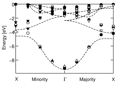
Figure 2: Band structure of Ni (minority and majority spin) as obtained from the linearization procedure of the GW+DMFT self-energy described in the text (dots) in comparison to the LDA band structure (dashed lines) and the experimental data of Bünemann et al. (2002) (triangles down) and Mårtensson and Nilsson (1984) (triangles up).

We now discuss further the simplifications made in our implementation. Because of the static approximation (iii), we could not implement self-consistency on $W_{loc}$ (Eq. (13)). We chose the value of ${\cal U}(\omega=0)$ ($\simeq 3.2eV$) by calculating the correlation function $\chi$ and ensuring that Eq. (11) is fulfilled at $\omega=0$, given the GW value for $W_{loc}(\omega=0)$ ($\simeq 2.2eV$ for Nickel Springer and Aryasetiawan (1998)). This procedure emphasizes the low-frequency, screened value, of the effective interaction. Obviously, the resulting impurity self-energy $\Sigma_{imp}$ is then much smaller than the local component of the GW self-energy (or than $V_{xc}^{loc}$), especially at high frequencies. It is thus essential to choose the second term in (First principles approach to the electronic structure of strongly correlated systems: combining GW and DMFT) to be the onsite component of the GW self-energy rather than the r.h.s of Eq. (10). For the same reason, we included $V_{xc}^{loc}$ in Eq.(First principles approach to the electronic structure of strongly correlated systems: combining GW and DMFT) (or, said differently, we implemented a mixed scheme which starts from the LDA Hamiltonian for the local part, and thus still involves a double-counting correction). We expect that these limitations can be overcome in a self-consistent implementation with a frequency-dependent ${\cal U}(\omega)$ (hence fulfiling Eq. (10)). In practice, it might be sufficient to replace the local part of the GW self-energy by $\Sigma_{imp}$ for correlated orbitals only. Alternatively, a downfolding procedure could be used.

In conclusion, we have proposed an ab initio dynamical mean field approach for calculating the electronic structure of strongly correlated materials, which combines GW and DMFT. The scheme aims at avoiding the conceptual problems inherent to “LDA+DMFT” methods, such as double counting corrections and the use of Hubbard parameters assigned to correlated orbitals. A full practical implementation of the GW$+$DMFT scheme is a major goal for future research, which requires further work on impurity models with frequency-dependent interaction parameters Motome and Kotliar (2000); Freericks et al. (1993); Sun and Kotliar (2002) as well as studies of various possible self-consistency schemes.