Effects of nonlinear sweep in the Landau-Zener-Stueckelberg effect

Abstract

We study the Landau-Zener-Stueckelberg (LZS) effect for a two-level system with a time-dependent nonlinear bias field (the sweep function) $W(t)$. Our main concern is to investigate the influence of the nonlinearity of $W(t)$ on the probability $P$ to remain in the initial state. The dimensionless quantity $\varepsilon=\pi\Delta^{2}/(2\hbar v)$ depends on the coupling $\Delta$ of both levels and on the sweep rate $v$. For fast sweep rates, i.e., $\varepsilon\ll 1,$ and monotonic, analytic sweep functions linearizable in the vicinity of the resonance we find the transition probability $1-P\cong\varepsilon(1+a)$, where $a>0$ is the correction to the LSZ result due to the nonlinearity of the sweep. Further increase of the sweep rate with nonlinearity fixed brings the system into the nonlinear-sweep regime characterized by $1-P\cong\varepsilon^{\gamma}$ with $\gamma\neq 1,$ depending on the type of sweep function. In case of slow sweep rates, i.e., $\varepsilon\gg 1$, an interesting interference phenomenon occurs. For analytic $W(t)$ the probability $P=P_{0}e^{-\eta}$ is determined by the singularities of $\sqrt{\Delta^{2}+W^{2}(t)}$ in the upper complex plane of $t$. If $W(t)$ is close to linear, there is only one singularity, that leads to the LZS result $P=e^{-\varepsilon}$ with important corrections to the exponent due to nonlinearity. However, for, e.g., $W(t)\propto t^{3}$ there is a pair of singularities in the upper complex plane. Interference of their contributions leads to oscillations of the prefactor $P_{0}$ that depends on the sweep rate through $\varepsilon$ and turns to zero at some $\varepsilon$. Measurements of the oscillation period and of the exponential factor would allow to determine $\Delta,$ independently.

I
Introduction

We will study the Landau-Zener-Stueckelberg (LZS) problem of quantum-mechanical transitions between the levels of a two-level system at the avoided level crossing (see Fig. 1) caused by the time dependence of the Hamiltonian lan32 ; zen32 ; stu32 ; akusch92 ; dobzve97

$$\widehat{H}=-\frac{1}{2}W(t)\sigma_{z}+\frac{1}{2}\Delta\sigma_{x},$$ (1)

where $\sigma_{\alpha},$ $\alpha=x,y,z$ are the Pauli matrices and

$$W(t)\equiv E_{1}(t)-E_{2}(t)$$ (2)

is the time-dependent bias of the two bare ($\Delta=0)$ energy levels. Because of its generality, the LZS problem is pertinent to many areas of physics. In particular, the time-dependent model of Eq. (1) is a simplification of the two-channel scattering problem with the curve crossing in the theory of molecular collisions (see, e.g., Refs. chi74, ; nak02, and references therein). An appropriate choice of $W(t)$, including oscillative time dependences, groditjunhae91 ; kay93 ; kay94 ; miysairae98 ; ternak98 may allow to manipulate the evolution of the system in a controlled way.groditjunhae91 ; ternak98 ; garsch02 The most important case is probably that of the linear energy sweep:

$$W(t)=vt,\qquad v={\rm const>0}$$ (3)

that can be solved exactly. If the system at $t\rightarrow-\infty$ was in the bare ground state $\psi_{1}=|\downarrow\rangle$ before crossing the resonance, the probability to stay in this state after crossing the resonance at $t\rightarrow\infty$  is given by zen32 ; stu32 ; dobzve97

$$P(\infty)\equiv P=e^{-\varepsilon},\qquad\varepsilon\equiv\frac{\pi\Delta^{2}}{2\hbar v}$$ (4)

for all $\varepsilon$.LZFoot Solution of the LZS problem with linear sweep for a general initial condition (the complete scattering matrix) and for multilevel systems can be found in Refs. nak87, ; poksin00, .

\begin{picture}(11.0,6.0)\centerline{\hbox{\psfig{angle=-90,width=256.0748pt}}} \end{picture}

Figure 1: A pair of tunnel-splitted levels vs. energy bias $W(t)$. Here $E_{1}$ and $E_{2}$ are the bare energy levels ($\Delta=0$), whereas $E_{\pm}$ are the exact adiabatic energy levels of Eq. (23). $P$ denotes the probability to remain in the (bare) state 1 after crossing the resonance.

Arguing that a typical smooth sweep function $W(t)$ crossing the resonance only one time can be linearized close to the resonancelanlif3 ; dobzve97 ; poksin00 and that the $t$-dependence of $W(t)$ far enough from the resonance does not matter, the LZS problem has been in most cases solved for linear sweeps $W(t)=vt$ (see, however, Ref. ternak97, ). Recently, however, there has been a great deal of interest to the LZS effect in systems of interacting tunneling species (see, e.g., Ref. hamraemiysai00, ) initiated by experiments on molecular magnets.weretal00epl In Ref. hamraemiysai00, the LZS effect has been investigated for an interacting system of $N$ particles with spin $S=1/2$. Since in this model each spin interacts with all the others with the same coupling constant, one can use a mean-field approach which becomes exact for $N\rightarrow\infty$. Therefore in general the effective field becomes nonlinear in time, due to the nonlinear $t$-dependence of the field on a given spin acting from other spins.

It is thus of principal interest to investigate the two-level Landau-Zener-Stueckelberg problem for a nonlinear energy sweep. First, for a weakly nonlinear sweep there will be corrections to Eq. (4) that should be especially pronounced in the slow-sweep region $\varepsilon\gg 1.$ Since an experimental realization of a linear sweep can only be approximate it is important to determine these corrections. Second, essentially nonlinear sweeps, including those with multiple crossing the resonance, are becoming technically feasible for such objects as magnetic molecules, where the Hamiltonian can be easily tuned by the external magnetic field (see, e.g., Ref. werses99, ). These nonlinear energy sweeps could be used to manipulate the system in a desired way, say to ensure $P=0$ for the finite sweep rates.

In our recent Letter garsch02 we have solved the inverse Landau-Zener-Stueckelberg problem, i.e., we have found such sweep functions $W(t)$ that ensure the required time-dependent probabilities $P(t)$ to stay in the initial state. Among the solutions are those corresponding to the time-symmetric $P(t)$ satisfying $P(-\infty)=1$ and $P(\infty)\equiv P=0.$ The functions $W(t)$ are more complicated than corresponding $P(t)$ and they become cumbersome for more sophisticated forms of $P(t).$ An interesting task is to find general criteria for the complete conversion $\psi_{1}\rightarrow\psi_{2},$ i.e., for $P=0,$ for the direct LZS problem and to apply it to the simplest nonlinear forms of $W(t).$ This is a further aim of our paper. We will obtain analytical solutions for fast and slow sweep as well as numerical solutions in the whole range of parameters.

The outline of the paper is as follows. In the next section we will describe the LZS problem  for a general sweep. Sec. III contains the discussion of the fast sweep, whereas results for slow sweep are presented in Sec. IV. We will show that in the slow-sweep case different kinds of singularities that characterize $W(t)$ sensitively influence the propability $P.$ The final section contains a summary and some conclusions.

For numerical calculation throughout the paper we use Wolfram Mathematica 4.0 that employs a very accurate differential equation solver needed for dealing with strongly oscillating solutions over large time intervals.

II LZS problem for general sweep

The Schrödinger equation for the coefficients of the wave function $\psi(t)=c_{1}(t)\psi_{1}+c_{2}(t)\psi_{2}$ can be written as

$$i\hbar\frac{d}{dt}\tilde{c}_{1}(t) = \frac{\Delta}{2}\tilde{c}_{2}(t),$$

$$i\hbar\frac{d}{dt}\tilde{c}_{2}(t) = -W(t)\tilde{c}_{2}(t)+\frac{\Delta}{2}\tilde{c}_{1}(t),$$ (5)

where $\tilde{c}_{1,2}(t)\equiv c_{1,2}(t)\exp\left[-\frac{i}{2\hbar}\int_{-\infty}^{t}dt^{\prime}W(t^{\prime})\right]$ satisfy the initial conditions

$$\tilde{c}_{1}(-\infty)=1,\qquad\tilde{c}_{2}(-\infty)=0,$$ (6)

and $W(t)\equiv E_{1}(t)-E_{2}(t)$ satisfies $W(-\infty)=-\infty$. A general nonlinear sweep function $W(t)$ can be parametrized as follows

$$W(t)=\Delta w(u),\qquad u\equiv vt/\Delta.$$ (7)

The corresponding dimensionless form of Eq. (5) is

$$\tilde{c}_{1}^{\prime}(u) = -\frac{i\tilde{\varepsilon}}{2}\tilde{c}_{2}(u),$$

$$\tilde{c}_{2}^{\prime}(u) = i\tilde{\varepsilon}w(u)\tilde{c}_{2}(u)-\frac{i\tilde{\varepsilon}}{2}\tilde{c}_{1}(u)$$ (8)

where ^′ denotes differentiation with respect to $u$ and the sweep-rate parameter $\tilde{\varepsilon}$ is defined by

$$\tilde{\varepsilon}\equiv\frac{\Delta^{2}}{\hbar v}=\frac{2}{\pi}\varepsilon.$$ (9)

(The reader should not confuse $\tilde{\varepsilon}$ and $\varepsilon$ that differ by a numerical factor; Whereas $\tilde{\varepsilon}$ arises in a natural way, $\varepsilon$ is used to represent most of the final results.)

It is convenient to represent dimensionless analytical functions $w(u)$ that behave linearly near $u=0$ in the form

$$w(u)=\alpha^{-1}f(\alpha u)\cong u+\frac{\alpha}{2!}f_{0}^{\prime\prime}u^{2}+\frac{\alpha^{2}}{3!}f_{0}^{\prime\prime\prime}u^{3}+\ldots$$ (10)

where $f_{0}^{\prime}=1$ and, in general, $f_{0}^{\prime\prime}\sim f_{0}^{\prime\prime\prime}\sim 1$. Whereas $v$ in Eq. (7) stands for the sweep rate, the parameter $\alpha$ in (10) controls the nonlinearity of the sweep. Below we will work out explicit results for the analytical sweep function

$$w(u)=\alpha^{-1}\sinh(\alpha u)$$ (11)

that satisfies $w(-u)=-w(u)$. A more general  analytical sweep function is

$$w(u)=\frac{1}{\alpha+\beta}\left(e^{\alpha u}-e^{-\beta u}\right)$$ (12)

that is characterized by $w(-u)\neq-w(u)$ for $\alpha\neq\beta.$ An interesting property of the corresponding LZS problem is that for $\alpha\neq\beta$ interchanging $\alpha$ and $\beta$ leads to essentially different solutions of the corresponding Schrödinger equation while $P$ being the same in both cases. This can be proven by considering the general scattering matrix of the problem, similarly to the proof of the reflection and transmission coefficients for scattering on a nonsymmetric one-dimensional potential being the same for both directions of the ongoing particle.lanlif3

Also we would like to consider nonanalytical sweep functions like the power-law $w(u)=u^{\alpha}$ with $\alpha>0.$  It is convenient to put this problem into a more general form and to introduce crossing and returning sweeps

$$w(u)=\left\{\begin{array}[]{ll}{\rm sign}(u)|u|^{\alpha},&\text{crossing}\\ -|u|^{\alpha},&\text{returning.}\end{array}\right.$$ (13)

Note that returning sweeps (with double crossing the resonance) are naturally realized in atomic and molecular collisions where the distance between the colliding species at first decreases and than increases again. stu32

III Fast sweep

In this section we will discuss the behavior of $P$ for fast sweep for which the propability $P$ should stay close to 1. The form of Eq. (8) is convenient to perform the fast-sweep approximation $\tilde{\varepsilon}\ll 1.$ In zeroth order of the perturbation theory one has $\tilde{c}_{1}(u)=1$ which can be used to obtain $\tilde{c}_{2}(u)$ from the second line of Eq. (8). The resulting equation for $\tilde{c}_{2}(u)$ can easily be solved. Using this result, the probability to stay in the initial state 1 can be expressed as

$$P\cong 1-|\tilde{c}_{2}(\infty)|^{2}$$

$$=1-\frac{\tilde{\varepsilon}^{2}}{4}\left|\int_{-\infty}^{\infty}du\exp\left[-i\tilde{\varepsilon}\int_{0}^{u}du^{\prime}w(u^{\prime})\right]\right|^{2}.$$ (14)

One can see that this is not a standard perturbation theory that would yield a correction of order $\tilde{\varepsilon}^{2}$ to $P.$ The integral over $u$ in Eq. (14) assumes large values for $\tilde{\varepsilon}\ll 1$ and is in general non-analytic in $\tilde{\varepsilon}.$ Since $u\sim u_{\varepsilon}\sim\varepsilon^{-1/2}\gg 1$ contribute to this integral for $\tilde{\varepsilon}\ll 1,$ the latter is very sensitive to the nonlinearity of $w(u).$ For weakly-nonlinear $w(u)$ that can be expanded into the Taylor series of Eq. (10) one has

$$\int_{0}^{u}duw(u)\cong\frac{1}{2!}u^{2}+\frac{\alpha}{3!}f_{0}^{\prime\prime}u^{3}+\frac{\alpha^{2}}{4!}f_{0}^{\prime\prime\prime}u^{4}+\ldots$$

If $\alpha\ll u_{\varepsilon}^{-1}\sim\tilde{\varepsilon}^{1/2},$ it is the first term of this expansion that is dominating. One can transform this condition into the dimensional form if one writes $W(t)\cong\dot{W}_{0}t+\ddot{W}_{0}t^{2}/2!+\ldots$ and makes comparison with Eq. (10). This yields the weak-nonlinearity condition

$$\alpha\ll\tilde{\varepsilon}^{1/2}\qquad\Longleftrightarrow\qquad\hbar\ddot{W}_{0}^{2}\ll\dot{W}_{0}^{3}.$$ (15)

With the help of Eqs. (7) and (9) one can establish that the LZS transition takes place not in the range $W(t)\cong vt\sim\Delta$ around the resonance, as could be expected, but in the much wider range

$$W(t)\sim\Delta/\sqrt{\tilde{\varepsilon}}=\sqrt{\hbar v}\gg\Delta$$ (16)

for the fast sweep. In the weakly nonlinear regime the main contribution to the integral in Eq. (14) stems from $u\sim u_{\varepsilon}$ and one obtains

$$P\cong 1-\varepsilon\left\{1+\left[\frac{\pi}{32}\left(f_{0}^{\prime\prime\prime}-\frac{5}{3}f_{0}^{\prime\prime 2}\right)\right]^{2}\left(\frac{\alpha^{2}}{\varepsilon}\right)^{2}\right\}.$$ (17)

Since $\alpha^{2}\ll\varepsilon,$ the leading-order result for $P$ does not depend on the nonlinearity, as expected. But Eq. (17) also demonstrates that the next-to-leading order in the nonlinearity reduces the probability $P,$ independently on whether the sweep function $w(u)$ [or $W(t)$] grows slower or faster than linear, in contrast to the expectation. This effect that dependes on $f_{0}^{\prime\prime}$ and $f_{0}^{\prime\prime\prime}$ can be rather small, though (see Fig. 2).

If $\alpha\gg\varepsilon^{1/2}$ and $w(u)$ is a power series that terminates at finite order $u^{n},$ then it is this latter term that dominates, and the main contribution to the integral in Eq. (14) comes from $u_{\varepsilon}\sim{\varepsilon}^{-1/(n+1)}$ that yields

$$1-P\sim\left(\varepsilon/\alpha^{2}\right)^{2n/(n+1)}.$$ (18)

The range of the energy bias $W(t)$ that is responsible for tunneling is given by

$$W(t)\sim\Delta/{\varepsilon}^{n/(n+1)}\gg\Delta$$ (19)

[cf. Eq. (16)].

A particular case of the above is the crossing power-law sweep described by Eq. (13) that contains the linear sweep as a particular case. Here one has $\int_{0}^{u}duw(u)=|u|^{\alpha+1}/(\alpha+1)$  and Eq. (14) yields

$$P\cong 1-\Gamma^{2}\left(\frac{1}{1+\alpha}\right)\left(\frac{\tilde{\varepsilon}}{1+\alpha}\right)^{2\alpha/(1+\alpha)},$$ (20)

where $\Gamma(x)$ is the gamma function. In the case $\alpha=1$ the familiar expansion $P\cong 1-\varepsilon$ of Eq. (4) for $\varepsilon\ll 1$ is recovered. For $\alpha>1$ the transition probability $1-P$ is smaller than that for the linear sweep. The opposite result is obtained for $\alpha<1,$ e.g., $1-P\propto\sqrt{\tilde{\varepsilon}}$ for $\alpha=1/3.$ For the returning power-law sweep of Eq. (13) one has $\int_{0}^{u}duw(u)=-{\rm sign}(u)|u|^{\alpha+1}/(\alpha+1)$ and the result has the form

$$P\cong 1-\Gamma^{2}\left(\frac{1}{1+\alpha}\right)\cos^{2}\left(\frac{\pi}{2(1+\alpha)}\right)\left(\frac{\tilde{\varepsilon}}{1+\alpha}\right)^{2\alpha/(1+\alpha)}.$$ (21)

\begin{picture}(11.0,6.0)\centerline{\hbox{\psfig{angle=-90,width=256.0748pt}}} \end{picture}

Figure 2: Dependence of the transition probability $1-P$ on the nonlinearity parameter $\alpha$ for the sweep function $w(u)=\alpha^{-1}\sinh(\alpha u)$ in the fast-sweep regime, $\varepsilon\ll 1$. The dashed lines are the asymptotes of Eqs.  (17) and (22).

For the sweep described by Eq. (11) one has $\int_{0}^{u}duw(u)=(\cosh\alpha u-1)/\alpha^{2}.$ In the case $\alpha^{2}\ll\tilde{\varepsilon}$ Eq. (14) yields the well known result for the linear sweep $P\cong 1-\varepsilon,$ as it should be for small enough nonlinearity. In the opposite case one can use the approximation $\int_{0}^{u}du^{\prime}w(u^{\prime})\cong e^{\alpha u}/(2\alpha^{2})$ to obtain

$$P\cong 1-\frac{\tilde{\varepsilon}^{2}}{\alpha^{2}}\left(\ln\frac{2\alpha^{2}}{\tilde{\varepsilon}}-\gamma\right)^{2},\qquad\tilde{\varepsilon}\ll\alpha^{2},$$ (22)

where $\gamma=0.577216.$ This is in accord with Eq. (18) in the limit $n\rightarrow\infty,$ up to the logarithm. The crossover between the linear and nonlinear regimes for the sweep function of Eq. (11) on $\alpha/\sqrt{\varepsilon}$ is shown in Fig. 2.

IV Slow sweep

In this section we will study the asymptotic behavior of $P$ for $\varepsilon\gg 1,$ i.e., for slow sweeps. This behavior will strongly depend on the analytical properties of $w(u).$ Let us first describe the general situation in case of slow sweep.

IV.1 General

It is convenient to solve the Schrödinger equation in the adiabatic basis formed of the states $\psi_{\pm}(t)$ that are solutions of the stationary Schrödinger equation at the time $t$. The evolution of the system nearly follows the lowest, i.e., $E_{-}(t),$ of the adiabatic energy levels (see Fig. 1)

$$E_{\pm}(t)=\pm\frac{1}{2}\Omega(t)=\pm\frac{1}{2}\sqrt{W^{2}(t)+\Delta^{2}},$$ (23)

whereas the probability of the transition to the upper level $E_{+}$ is small. The explicit form of the adiabatic states is garsch02

$$\psi_{\pm}(t)=\frac{1}{\sqrt{2}}\left[\pm K_{\pm}(t)\psi_{1}+K_{\mp}(t)\psi_{2}\right],$$

where $K_{\pm}(t)\equiv\sqrt{1\pm W(t)/\Omega(t)}.$ Writing the wave function in the form $\psi=c_{+}(t)\psi_{+}(t)+c_{-}(t)\psi_{-}(t)$ one obtains the equations for $\tilde{c}_{\pm}(t)\equiv\exp\left(i\int dtE_{-}(t)/\hbar\right)c_{\pm}(t).$ The dimensionless form of these equations reads [see Eq. (7)]

$$\tilde{c}_{-}^{\prime}(u)=\frac{w^{\prime}(u)}{2\overline{\Omega}^{2}(u)}\tilde{c}_{+}(u),\qquad\overline{\Omega}(u)\equiv\sqrt{1+w^{2}(u)}$$

$$\tilde{c}_{+}^{\prime}(u)=-i\tilde{\varepsilon}\overline{\Omega}(u)\tilde{c}_{+}(u)-\frac{w^{\prime}(u)}{2\overline{\Omega}^{2}(u)}\tilde{c}_{-}(u)$$ (24)

and the initial condition is $\tilde{c}_{-}(-\infty)=1,$ $\tilde{c}_{+}(-\infty)=0.$ The probability $\ P$ to stay in state 1 is given by

$$P=\left\{\begin{array}[]{ll}|\tilde{c}_{+}(\infty)|^{2},&\text{crossing}\\ |\tilde{c}_{-}(\infty)|^{2}=1-|\tilde{c}_{+}(\infty)|^{2},&\text{returning}\end{array}\right.$$ (25)

and it is small for crossing sweeps and close to 1 for returning sweeps. In fact, for returning sweeps $P$ tends to 1 in the limits of both fast and slow sweeps, as is illustrated in Fig. 3. Indeed, from Fig. 1 one can see that for a fast sweep the system practically remains on the bare level $E_{1}$, whereas for a slow sweep it travels along the adiabatic level $E_{-}$ and thus returns to $E_{1}$ for $W(\infty)=-\infty$.

One possible way of solving Eq. (7) is to transform it to a single second-order differential equation and then to apply the WKB approximation to the corresponding overbarrier-reflection problem with a complex potential. The result is a linear combination of two solutions that can be interpreted as ongoing and reflected waves. Then the (exponentially small) factor in front of the reflected-wave solution can be found from the analysis of Stokes lines in the complex plane (see, e.g., Ref. nak02, and references therein). This analysis is rather involved, however. Below we will present an alternative and more simple method of solving Eq. (7) that does not rely on the WKB approximation.

One can immediately write down the formal solution of Eq. (7) for $|\tilde{c}_{+}(\infty)|^{2}$ that contains yet to be determined $\tilde{c}_{-}(u)$

$$|\tilde{c}_{+}(\infty)|^{2}=\left|\frac{1}{2}\int_{-\infty}^{\infty}du\frac{w^{\prime}(u)}{\overline{\Omega}^{2}(u)}\tilde{c}_{-}(u)\exp\left[i\tilde{\varepsilon}\Phi(u)\right]\right|^{2}$$ (26)

with

$$\Phi(u)\equiv\int_{0}^{u}du^{\prime}\,\overline{\Omega}(u^{\prime}).$$ (27)

Since for the slow sweep $\tilde{c}_{-}(u)$ remains close to 1, $\tilde{c}_{-}(u)\Rightarrow 1$ is a reasonable approximation. We will see below that this approximation is sufficient to obtain the correct exponential in the exponentially small $P$, as well as the prefactor with better than 10% accuracy. On the top of it, the approximation will be refined to obtain the exact prefactor. The asymptotic $\tilde{\varepsilon}$ dependence of the rhs of Eq. (26) depends strongly on the analytical properties of $\Phi(u).$ Even if $w(u)$ is chosen to be an analytical function, the integrand $\overline{\Omega}(u)$ in Eq. (27) is not analytical but has singularities at the branch points at which $w^{2}(u)=-1.$ We will see that these singularities determine the large-$\varepsilon$ dependence of $P,$ for analytical sweep functions $w(u).$

IV.2 Non-analytic sweep functions

We consider for the beginning the simpler case of sweep functions that are non-analytic at cros$\sin$g the resonance, $u=0,$ namely the power-law sweep functions of Eq. (13) with a general $\alpha.$ For $\tilde{\varepsilon}\gg 1$ the integral in Eq. (26) with $\tilde{c}_{-}(u)\Rightarrow 1$ is dominated by small $u$ for which $w(u)\ll 1,$ and thus $\overline{\Omega}(u)\cong 1.$ After taking advantage of the symmetry of Eq. (13) it simplifies to

$$|\tilde{c}_{+}(\infty)|^{2}=\mathrel{\mathop{\lim}\limits_{\delta\rightarrow 0}}\left|\int_{0}^{\infty}du\,e^{-\delta u}\alpha u^{\alpha-1}\left\{\begin{array}[]{l}\cos\left(\tilde{\varepsilon}u\right)\\ \sin(\tilde{\varepsilon}u)\end{array}\right\}\right|^{2}$$

for crossing and returning sweeps, respectively. The final result for $P$ of Eq. (25) reads

$$P\cong\left\{\begin{array}[]{ll}\displaystyle\frac{\Gamma^{2}(1+\alpha)}{\tilde{\varepsilon}^{2\alpha}}\cos^{2}\left(\frac{\pi\alpha}{2}\right),&\text{crossing}\\ \displaystyle 1-\frac{\Gamma^{2}(1+\alpha)}{\tilde{\varepsilon}^{2\alpha}}\sin^{2}\left(\frac{\pi\alpha}{2}\right),&\text{returning.}\end{array}\right.$$ (28)

The nonanalytic $\varepsilon$ dependent contribution here stems from the nonanalytic behavior of $w(u)$ at $u=0$ and it vanishes for analytic functions such as $w(u)=u$ or $w(u)=u^{3}$ for the crossing sweep and $w(u)=u^{2}$ for the returning sweep. Numerical results for $P(\varepsilon)$ along with the asymptotes of Eqs. (20), (21), and (28) are shown for $\alpha=1/2$ and $\alpha=1$ in Fig. 3. One can see that the slow-sweep asymptote of Eq. (28) works well starting from relatively low values of $\varepsilon$ for crossing sweeps and from larger $\varepsilon$ for returning sweeps. $P(\varepsilon)$ for $\alpha=1,2,3,4$ and $5$ are shown in Fig. 4. In this case the asymptotes of Eq. (28) require rather large values of $\varepsilon$ and they can be seen on the log plot only (see Fig. 5) With increasing $\alpha$ oscillations of $P(\varepsilon)$ develop; the reason for this will be explained below.

\begin{picture}(11.0,6.0)\centerline{\hbox{\psfig{angle=-90,width=256.0748pt}}} \end{picture}

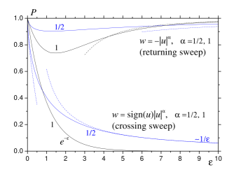
Figure 3: Staying probability $P(\varepsilon)$ for power-law sweep functions with exponents $\alpha=1/2$ and $\alpha=1$. Solid lines are numerical results and dashed lines are some of the analytical asymptotes.

\begin{picture}(11.0,6.0)\centerline{\hbox{\psfig{angle=-90,width=256.0748pt}}} \end{picture}

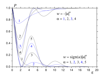
Figure 4: $P(\varepsilon)$ for power-law sweep functions with exponents $\alpha=1,2,3,4$ and $5$.

\begin{picture}(11.0,6.0)\centerline{\hbox{\psfig{angle=-90,width=256.0748pt}}} \end{picture}

Figure 5: $P(\varepsilon)$ for crossing power-law sweep functions with exponents $\alpha=1.5,2$ and $2.5$. Dashed lines are high-$\varepsilon$ asymptotes of Eq. (28).

IV.3 Analytic sweep functions

As we will see, the form of the probability $P$ for $\varepsilon\gg 1$ crucially depends on the number of singularities of $\overline{\Omega}(u)=\sqrt{1+w^{2}(u)}$ in the upper complex plane. In the next subsection we will discuss sweep functions $w(u)$ for which there is only one singularity, starting from the weakly nonlinear case. For strongly nonlinear sweep with retardation in the resonance region, there is a pair of singularities symmetric with respect to the imaginary axis, that dominate $P$ for $\varepsilon\gg 1$. In this case $P$ can be represented in the form of a small exponential with a prefactor oscillating as a function of $\varepsilon$.

IV.3.1 One singularity: Exponent

For analytic sweep functions $w(u)$ the value of $|\tilde{c}_{+}(\infty)|^{2}$ given by Eq. (26) is exponentially small for $\tilde{\varepsilon}\gg 1,$ and it is defined by the singularities of the integrand in the upper complex half-plane that are closest to the real axis. These singularities are combinations of poles and branching points at $w^{2}(u)=w_{c}^{2}=-1.$ Let us consider at first sweep functions $w(u)$ that are monotonic and close to the linear function, $w(u)$ $\approx u.$ In this case there is only one singularity at $u\approx w(u)=w_{c}=i,$ and it is convenient to use $w$ as the sweep variable instead of $u$ in Eq. (26):

$$P\cong\left|\frac{1}{2}\int_{-\infty}^{\infty}\frac{dw}{\overline{\Omega}^{2}(w)}\tilde{c}_{-}(w)e^{i\tilde{\varepsilon}\Phi(w)}\right|^{2}$$

$$\Phi(w)\equiv\int_{0}^{w}dw\frac{du(w)}{dw}\overline{\Omega}(w).$$ (29)

We deform the integration line into the contour ${\cal C}$ that goes down along the left side of the cut $[i,i\infty],$ then around the pole at $w=i,$ and finally along the right side of the cut to $i\infty.$ Then the phase $\Phi(w)$ can be written in the form

$$\Phi(w)=\Phi_{c}+\delta\Phi(w)$$

$$\Phi_{c}=\int_{0}^{i}dw\frac{du(w)}{dw}\overline{\Omega}(w)=i\int_{0}^{1}dy\,u^{\prime}(y)\sqrt{1-y^{2}}$$

$$\delta\Phi(y)=i\int_{1}^{y}dy\,u^{\prime}(y)\sqrt{1-y^{2}},\qquad w=iy.$$ (30)

Accordingly the result of integration in Eq. (29) can be represented in the form

$$P=P_{0}e^{-\eta},\qquad\eta=2\tilde{\varepsilon}\mathop{\rm Im}\Phi_{c},$$ (31)

where the prefactor $P_{0}$ follows from

$$P_{0}=\left|\frac{1}{2}\int_{{\cal C}}\frac{dy}{1-y^{2}}\tilde{c}_{-}(y)e^{i\tilde{\varepsilon}\delta\Phi(y)}\right|^{2}.$$ (32)

Large values of $\tilde{\varepsilon}$ in our case ensure exponential smallness of $P$ in Eq. (31). Let us at first calculate the exponent $\eta$ for a weakly-nonlinear sweep described by Eq. (10). Inverting Eq. (10) for $\alpha\ll 1$ one obtains

$$u^{\prime}(y)\cong 1-i\alpha f_{0}^{\prime\prime}y+\frac{\alpha^{2}}{2}\left[f_{0}^{\prime\prime\prime}-3\left(f_{0}^{\prime\prime}\right)^{2}\right]y^{2}$$

and accordingly

$$\eta=2\tilde{\varepsilon}\mathop{\rm Im}\Phi_{c}\cong\varepsilon\left\{1+\frac{\alpha^{2}}{8}\left[f_{0}^{\prime\prime\prime}-3\left(f_{0}^{\prime\prime}\right)^{2}\right]\right\}.$$ (33)

For the time-antisymmetric sweep, $W(-t)=-W(t),$ one has $f_{0}^{\prime\prime}=0.$ Then for $f_{0}^{\prime\prime\prime}>0$ the exponent $\eta$ increases and the probability $P$ to stay in state 1 decreases. This result seems counterintuitive since in this case the system spends less time in the vicinity of the resonance than in the case of a linear sweep and one could expect that $P$ should increase. In fact, however, for a slow sweep the (small) probability to occupy state (+) oscillates many times during the resonance crossing and thus decreasing of $P$ is a coherence effect that cannot be explaned by simple kinetic arguments.

IV.3.2 One singularity: Prefactor

Now we turn to the calculation of the prefactor $P_{0}$ in Eq. (31) setting $\tilde{c}_{-}(y)\Rightarrow 1$ in Eq. (32) [see comment below Eq. (27)]. For $\tilde{\varepsilon}\gg 1$ the values of $y$ in the vicinity of $1$ dominate the integrals. Thus one can introduce $t=y-1\ll 1$ and simplify Eq. (32) to

$$P_{0}\cong\left|\frac{1}{4}\int_{{\cal C}_{t}}\frac{dt}{t}\exp\left[\tilde{\varepsilon}u_{c}^{\prime}\sqrt{2}\frac{2}{3}(-t)^{3/2}\right]\right|^{2},$$ (34)

where $u_{c}^{\prime}\equiv u^{\prime}(1)$ and the contour ${\cal C}_{t}$ goes from $\infty$ to 0 above the cut $[0,\infty]$ around the pole at $t=0$ and then to $\infty$ below the cut. At the upper and lower sides of the cut one has $(-t)_{\pm}^{3/2}=\pm it^{3/2}.$ Thus Eq. (34) yields

$$P_{0} \cong \left|\frac{1}{4}\left[2\pi i-2i\int_{0}^{\infty}\frac{dt}{t}\sin\left(\tilde{\varepsilon}u_{c}^{\prime}\sqrt{2}\frac{2}{3}t^{3/2}\right)\right]\right|^{2}$$ (35)

$$= \left(\frac{\pi}{2}-\frac{\pi}{6}\right)^{2}=\left(\frac{\pi}{3}\right)^{2}\simeq 1.096.$$

Note that this prefactor is a number and it does not depend on the argument of sin, i.e., on $\tilde{\varepsilon}$ and on the constant $u_{c}^{\prime}$ that encapsulates the nonlinearity of the sweep. One can notice that this prefactor slightly deviates from the exact prefactor 1 for the linear sweep. zen32 ; dobzve97 This is the consequence of the approximation $\tilde{c}_{-}(w)\Rightarrow 1$ in Eq. (29).

The reason for that wrong prefactor of Eq. (35) is the following. Although $\tilde{c}_{-}(u)$ only slightly deviates from 1 along the real axis, it becomes singular at the relevant point $w=i$ in the complex plane. This singularity can be worked out and the prefactor can be corrected. To this end, we note that the solution of Eq. (24) for $\tilde{\varepsilon}\gg 1$ can be expanded in powers of $1/\tilde{\varepsilon}.$ This expansion captures only the analytical part of the solution that yields $P=0$ in all orders in $1/\tilde{\varepsilon}$ while the nonanalytic part of the solution that yields $P\sim e^{-\varepsilon}$ cannot be found by this method. Nevertheless, the $1/\tilde{\varepsilon}$ expansion is sufficient to determine $\tilde{c}_{-}(w)$ that enters Eq. (32) to correct the prefactor. So we write down the expansions for $\tilde{c}_{\pm}(w)$ in the form

$$\tilde{c}_{\pm}(w)=\sum_{n=0}^{\infty}\frac{\tilde{c}_{\pm,n}(w)}{\left(i\tilde{\varepsilon}\right)^{n}},$$ (36)

where $\tilde{c}_{-,n}(-\infty)=\delta_{n0},$ and $\tilde{c}_{+,n}(-\infty)=0.$ From Eq. (24) that can be rewritten in the form

$$\frac{d\tilde{c}_{-}(w)}{dw} = \frac{\tilde{c}_{+}(w)}{2\overline{\Omega}^{2}(w)},$$

$$\frac{d\tilde{c}_{+}(w)}{dw} = -i\tilde{\varepsilon}\frac{du(w)}{dw}\overline{\Omega}(w)\tilde{c}_{+}(w)-\frac{\tilde{c}_{-}(w)}{2\overline{\Omega}^{2}(w)}$$ (37)

follows the infinite set of equations ($u^{\prime}\equiv du(w)/dw$)

$$\frac{d\tilde{c}_{-,n}(w)}{dw} = \frac{\tilde{c}_{+,n}(w)}{2\overline{\Omega}^{2}}$$

$$\tilde{c}_{+,n}(w) = -\frac{1}{u^{\prime}\overline{\Omega}}\left[\frac{d\tilde{c}_{+,n-1}(w)}{dw}+\frac{\tilde{c}_{-,n-1}(w)}{2\overline{\Omega}^{2}}\right]$$ (38)

This set of equations can be solved recurrently:

$$\tilde{c}_{+,0}(w) = 0,\qquad\qquad\tilde{c}_{-,0}(w)=1,$$

$$\tilde{c}_{+,1}(w) = -\frac{1}{2u^{\prime}\overline{\Omega}^{3}},\qquad\tilde{c}_{-,1}=-\frac{1}{4}\int_{-\infty}^{w}\frac{dw^{\prime}}{u^{\prime}\overline{\Omega}^{5}},$$ (39)

etc. In Figs. 6a and 6b we compare the dependence $|\tilde{c}_{+}(w)|^{2}$ obtained by the numerical solution of Eq. (37) and that using the $n=1$ term of Eq. (36) with $\tilde{c}_{+,1}$ from Eq. (39)  for the linear sweep [$w(u)=u$] with $\varepsilon=15$. Whereas the agreement in the region $w\approx 0$ can be improved by taking into account further terms of Eq. (36), the corresponding smooth and even functions $|\tilde{c}_{+}(w)|_{{\rm pert}}^{2}$ do not yield the asymptotic value $P=|\tilde{c}_{+}(\infty)|^{2}$ at any order of $1/\tilde{\varepsilon}.$ The latter is due to the singular part of the solution that oscillates and tends to the exponentially small value $P=e^{-\varepsilon}$ [see Fig. 6b].

\begin{picture}(11.0,6.0)\centerline{\hbox{\psfig{angle=-90,width=256.0748pt}}} \end{picture}

\begin{picture}(11.0,6.0)\centerline{\hbox{\psfig{angle=-90,width=256.0748pt}}} \end{picture}

Figure 6: Lowest-order $1/\tilde{\varepsilon}$ expansion for $|\tilde{c}_{+}(w)|_{{\rm pert}}^{2}$ compared with the exact numerical solution. $a$-General view; $b$-Right-wing magnification.

To obtain the solution of the problem that is improved by use of the $1/\tilde{\varepsilon}$ expansion while not losing the singular contribution at $w\rightarrow\infty,$ one should substitute Eq. (36) into Eq. (29). After multiple integration by parts the latter takes up the form

$$P\cong\left|\frac{1}{2}\int_{-\infty}^{\infty}dw\,e^{i\tilde{\varepsilon}\Phi(w)}\sum_{n=0}^{\infty}\left(-u^{\prime}(w)\overline{\Omega}(w)\hat{I}\right)^{n}\frac{\tilde{c}_{-,n}(w)}{\overline{\Omega}^{2}(w)}\right|^{2},$$ (40)

$\hat{I}$ being the integration operator. The integration by parts eliminated the powers of $1/\tilde{\varepsilon}$ that are present in Eq. (36). On the other hands, it is clear that contributions of the terms with $n>0$ in Eq. (40) should be small for $\tilde{\varepsilon}\gg 1$ unless these terms have singularities at $w=i.$ These singularitities do exist, as can be seen from Eq. (39). So in the leading order in $1/\tilde{\varepsilon}$ it is sufficient to take into account only the most singular contributions in $\tilde{c}_{\pm n}(w)$ near $w=i$ that allows to simplify Eqs. (38) using

$$w = i+z,\qquad|z|\ll 1,$$

$$\qquad\overline{\Omega} \cong \sqrt{2iz},\qquad u^{\prime}=u_{c}^{\prime}={\rm const.}$$ (41)

Then Eqs. (38) become

$$\frac{d\tilde{c}_{-,n}(z)}{dz} = \frac{\tilde{c}_{+,n}(z)}{4iz}$$

$$\tilde{c}_{+,n}(z) = -\frac{1}{u_{c}^{\prime}\sqrt{2iz}}\left[\frac{d\tilde{c}_{+,n-1}(z)}{dz}+\frac{\tilde{c}_{-,n-1}(z)}{4iz}\right].$$ (42)

The solution of these equations can be searched in the form

$$\tilde{c}_{\pm,n}(z)=\left\{\begin{array}[]{c}i\\ 1\end{array}\right\}\frac{\beta_{\pm,n}}{(2i)^{n/2}\left(u_{c}^{\prime}\right)^{n}z^{3n/2}},$$ (43)

where the coefficients $\beta_{\pm,n}$ satisfy

$$-6n\beta_{-,n} = \beta_{+,n},\qquad\beta_{-0}=1$$

$$\beta_{+,n} = \frac{3}{2}(n-1)\beta_{+,n-1}+\frac{1}{4}\beta_{-,n-1}$$ (44)

and can be obtained recurrently. Under the same conditions, the sum in Eq. (40) simplifies to

$$\sum_{n=0}^{\infty}\left(-u^{\prime}\overline{\Omega}\hat{I}\right)^{n}\frac{\tilde{c}_{-,n}}{\overline{\Omega}^{2}}$$

$$\qquad{}\cong\sum_{n=0}^{\infty}\left(-u_{c}^{\prime}\sqrt{2iz}\hat{I}\right)^{n}\frac{\beta_{-,n}}{(2i)^{n/2+1}\left(u_{c}^{\prime}\right)^{n}z^{3n/2+1}}$$

$$\qquad{}=\frac{1}{2iz}\sum_{n=0}^{\infty}\left(\frac{2}{3}\right)^{n}\frac{\beta_{-,n}}{n!}=\frac{1}{2iz}\sum_{n=0}^{\infty}\delta_{n},$$ (45)

where we used $\hat{I}z^{a}=z^{a+1}/(a+1)$ and defined $\delta_{n}=(2/3)^{n}\beta_{-,n}/n!$ For $\delta_{n}$ one obtains from Eqs. (44) the recurrence relation

$$\delta_{n}=\left(1-\frac{5}{6n}\right)\left(1-\frac{7}{6n}\right)\delta_{n-1},\qquad\delta_{0}=1.$$

Its solution is

$$\delta_{n} = \prod_{k=1}^{n}\left(1-\frac{5}{6k}\right)\left(1-\frac{7}{6k}\right)$$

$$= \frac{\left(1/6\right)_{n}\left(-1/6\right)_{n}}{\left(n!\right)^{2}}=\frac{\left(1/6\right)_{n}\left(-1/6\right)_{n}}{\left(1\right)_{n}}\frac{1}{n!},$$

where $(a)_{n}\equiv\Gamma(n+a)/\Gamma(a).$ The sum $\sum_{n=0}^{\infty}\delta_{n}$ in Eq. (45) is a hypergeometric function of argument 1:

$$\sum_{n=0}^{\infty}\delta_{n} = \sum_{n=0}^{\infty}\left.\frac{\left(1/6\right)_{n}\left(-1/6\right)_{n}}{\left(1\right)_{n}}\frac{x^{n}}{n!}\right|_{x=1}$$

$$= \left.{}_{2}F_{1}(1/6,-1/6;1;x)\right|_{x=1}$$

$$= \frac{1}{\Gamma(1+1/6)\Gamma(1-1/6)}=\frac{3}{\pi}.$$

Note that the approximation $\tilde{c}_{-}(w)\Rightarrow 1$ in Eq. (29) that leads to Eq. (35) for the prefactor amounts to neglection of all the terms of this sum except for the zeroth term $\delta_{0}=1.$ Summing up all the most singular terms of the $1/\tilde{\varepsilon}$ expansion, as was done above, compensates for the wrong factor $(\pi/3)^{2}$ in Eq. (35) and renders the prefactor the correct value 1. This value of the prefactor is valid for both linear and nonlinear sweep, if $P$ is dominated by only one singularity in the complex plane. It is the consequence of cancelling of the quantity $u_{c}^{\prime}$, which describes the nonlinearity of the sweep, in Eqs. (35) and (45).

We thus have obtained the formula for the probability to stay in the initial unperturbed state 1 after a slow ($\tilde{\varepsilon}\gg 1$) energy sweep through the resonance

$$P\cong e^{-\eta},\qquad\eta=2\tilde{\varepsilon}\mathop{\rm Im}\Phi_{c},\qquad\Phi_{c}=\int^{u_{c}}du\overline{\Omega}(u),$$ (46)

where $\tilde{\varepsilon}$ is given by Eq. (9), $\overline{\Omega}(u)=\sqrt{1+w^{2}(u)}$ is the dimensionless energy gap at the avoided level crossing. Note that $\Phi_{c}$ does not depend on $\tilde{\varepsilon}.$ The integral in Eq. (46) is taken from the real axis to the singularity point $u_{c}$ in the upper complex plane that is defined by $\overline{\Omega}(u_{c})=0$. This formula can be found in the textbook by Landau and Lifshitz. lanlif3 Pokrovsky, Savvinykh, and Ulinich poksavuli58 showed for a similar problem of the overbarrier reflection of a quantum-mechanical particle that the prefactor is equal to 1, using a different method. For a weakly-nonlinear sweep described by Eq. (10) the exponent $\eta$ is given by Eq. (33). In contrast, as we have seen in Sec. IV.2, for non-analytic sweep functions $W(t)$ the result is not exponentially small and is given by Eq. (28) for a particular case of crossing and returning power-law sweep functions of Eq. (13).

IV.3.3 A pair of singularities

In many important cases the behavior of $P$ is more complicated than the well-known formula Eq. (46) does suggest. For essentially nonlinear time-antisymmetric (crossing) or symmetric (returning) sweep functions $W(t)$ typically there are two singularities at $u_{c\pm}$ in the upper complex plane that are closest to the real axis and symmetric with respect to the imaginary axis. It can be shown with the same method that $P$ has the form ($\tilde{\varepsilon}\gg 1$)

$$P\cong\left|e^{i\tilde{\varepsilon}\Phi_{c+}}+e^{i\tilde{\varepsilon}\Phi_{c-}}\right|^{2},\qquad\Phi_{c\pm}=\pm\Phi_{c}^{\prime}+i\Phi_{c}^{\prime\prime},$$ (47)

i.e., both contributions have prefactors 1. This is not surprising since for $\tilde{\varepsilon}\gg 1$ contributions from different singularities are well separated from each other and the method used above applies to each of them. Eq. (47) can be rewritten in the form

$$P\cong P_{0}e^{-\eta},\qquad P_{0}=4\cos^{2}\left(\tilde{\varepsilon}\Phi_{c}^{\prime}\right),\qquad\eta=2\tilde{\varepsilon}\Phi_{c}^{\prime\prime}$$ (48)

that contains an oscillating prefactor $P_{0}$ with $\Phi_{c}^{\prime}\sim$ $1,$ according to the definition of the phase $\Phi$ in Eq. (29). These results pertain to the crossing sweep. For the returning sweep one obtains

$$P\cong 1-P_{0}e^{-\eta}.$$ (49)

Turning the prefactor $P_{0}$ to zero for some (finite!) sweep rates is the so-called complete conversion from state 1 to state 2 that was mentioned in the introduction. In Ref. garsch02, we have found this phenomenon for specially chosen sweep functions $W(t)$ of a more complicated form. Here we demonstrated that the full conversion at finite sweep rates is a general phenomenon for a nonlinear sweep. Whereas an oscillating prefactor can be found in earlier publications (see, e.g., Ref. ternak97, ), here we have shown its simple relation to the relevant singularities of the LZS problem.

\begin{picture}(11.0,5.0)\centerline{\hbox{\psfig{angle=-90,width=256.0748pt}}} \end{picture}

Figure 7: Integration contour in the complex plane $u$ in Eq. (29) for the sweep function $w(u)=u^{3}$. A pair of singularities at $u=(\pm\sqrt{3}+i)/2$ dominate the probability $P$ for slow sweep, $\varepsilon\gg 1$.

IV.4
Particular cases

Let us now consider particular cases of the LZS effect with nonlinear energy sweep, which will allow to explore the role of the singularities in the prefactor in more detail. For the power-law sweeps of Eq. (13) with natural $\alpha=n$, such as $w(u)=u^{2},$ $w(u)=u^{3},$ etc., there are $n$ singularities in the upper complex plane at $u=u_{k}=\exp\left[i\pi(1/2+k)/n\right]$ with $k=0,1,\ldots,n-1$ (see Fig. 7 for $\alpha=3$). Closest to the real axis are those with $k=0$ and $k=n-1$. The integration contour in Fig. 7 goes along both sides of the cuts initiating at the singularity points. These cuts are chosen so that $\delta\Phi$ in Eq. (30) is real on both sides of the cut (i.e., the cuts are the so-called anti-Stokes lines), so that $P$ is determined by purely oscillating integrals. For all other directions of the cuts, one has exponentially converging integrals on one side of the cut but exponentially diverging integrals on another side of the cut. After calculation of $\Phi_{c}$ in Eq. (46) one obtains

$$\left\{\begin{array}[]{l}\Phi_{c}^{\prime}\\ \Phi_{c}^{\prime\prime}\end{array}\right\}=\left\{\begin{array}[]{l}\cos\frac{\pi}{2n}\\ \sin\frac{\pi}{2n}\end{array}\right\}2^{1/n}\frac{\Gamma^{2}\left(1+\frac{1}{2n}\right)}{\Gamma\left(2+\frac{1}{n}\right)}.$$ (50)

Note that for $n=1$ there is only one pole, and Eq. (50) yields $\Phi_{c}^{\prime}=0$ and $\eta=2\tilde{\varepsilon}\Phi_{c}^{\prime\prime}=(\pi/2)\tilde{\varepsilon}=\varepsilon,$ so that one returns to the LZS result $P=e^{-\varepsilon}.$ In other cases the prefactor $P_{0}$ like in Eqs. (48) and (49) oscillates and turns to zero at some values of the sweep rate, where contributions of the two singularities in Eq. (47) cancel each other. In the latter case, a complete Landau-Zener-Stueckelberg transition is achieved for crossing sweeps. We have shown the prefactor $P_{0}$ for $w=u^{3}$ in Fig. 8, where the solid line is $e^{\eta}P$ with numerically computed $P$ and $\eta=2\tilde{\varepsilon}\Phi_{c}^{\prime\prime}$ and the dashed line is the analytical result $P_{0}=4\cos^{2}\left(\tilde{\varepsilon}\Phi_{c}^{\prime}\right)$. It is seen that Eqs. (48) and (50) work well for large $\varepsilon$. Plotting $P_{0}$ reveals oscillations that are not seen at large $\varepsilon$ in Fig. 4.

\begin{picture}(11.0,6.0)\centerline{\hbox{\psfig{angle=-90,width=256.0748pt}}} \end{picture}

Figure 8: Prefactor $P_{0}$ in $P(\varepsilon)=P_{0}e^{-\eta}$ for power-law sweep function $w=u^{3}$. The solid line is $e^{\eta}P$ with numerically computed $P$ and $\eta=2\tilde{\varepsilon}\Phi_{c}^{\prime\prime}$ and the dashed line is the analytical result $P_{0}=4\cos^{2}\left(\tilde{\varepsilon}\Phi_{c}^{\prime}\right)$ [see Eqs. (48) and (50)].

\begin{picture}(11.0,6.0)\centerline{\hbox{\psfig{angle=-90,width=256.0748pt}}} \end{picture}

Figure 9: Real and imaginary parts of the quantum-mechanical phase $\Phi$ at symmetric singularities in the complex plane [see Eq. (47)] for the sweep function $w=\alpha^{-1}\sinh(\alpha u)$ vs $\alpha$, given by Eqs. (52) and (54).

\begin{picture}(11.0,6.0)\centerline{\hbox{\psfig{angle=-90,width=256.0748pt}}} \end{picture}

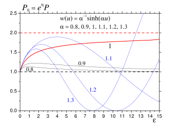
Figure 10: Prefactor $P_{0}$ in $P=P_{0}e^{-\eta}$ for the sweep function $w=\alpha^{-1}\sinh(\alpha u)$ defined as $P_{0}=e^{\eta}P$ with numerically computed $P$ for $\alpha$ in the vicinity of 1. The dotted lines at $P_{0}=1$ and at $P_{0}=2$ correspond to the analytical results for $\alpha<1$ and $\alpha=1$, respectively.

\begin{picture}(11.0,6.0)\centerline{\hbox{\psfig{angle=-90,width=256.0748pt}}} \end{picture}

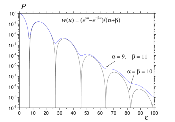
Figure 11: Staying probability $P$ vs the inverse sweep rate for the sweep with slightly broken antisymmetry $w(-u)=-w(u)$. For $\alpha=9$ and $\beta=11$ (same results for $\alpha=11$ and $\beta=9$) interference of the two poles closest to the real axis is not complete and $P$ does not turn to zero.

The next interesting case is that of the sinh sweep function of Eq. (11). This model allows to track the changes of $P$ as function of the continuous parameter $\alpha$ (which is the measure of nonlinearity) keeping the sweep function $w(u)$ analytical. The singularities depend on $\alpha.$ For $\alpha<1$ the singularity closest to the real axis is at

$$u=u_{c}=i\ \frac{\arcsin\alpha}{\alpha},$$ (51)

whereas the next singularity is at $u=i\left(\pi-\arcsin\alpha\right)/\alpha.$ Keeping only the singularity at $u_{c}$ for $\tilde{\varepsilon}\gg 1$ one obtains from Eq. (46)

$$\eta=\frac{2\tilde{\varepsilon}}{\alpha}{\bf E}\left(\arcsin\alpha,\frac{1}{\alpha^{2}}\right),\qquad(\alpha<1),$$ (52)

where ${\bf E}(\varphi,m)$ is the incomplete elliptic integral of second kind. In the region $\alpha>1$ there is a pair of singularities at

$$u=u_{c\pm}=\pm\frac{1}{\alpha}\ln\left(\sqrt{\alpha^{2}-1}+\alpha\right)+\frac{i\pi}{2\alpha}$$ (53)

that are closest to the real axis. In this case one obtains Eq. (48) with

$$\eta = \frac{2\tilde{\varepsilon}}{\alpha}{\bf E}\left(\frac{1}{\alpha^{2}}\right)$$

$$\Phi_{c}^{\prime} = \frac{1}{\alpha}\left[{\bf K}\left(1-\frac{1}{\alpha^{2}}\right)-{\bf E}\left(1-\frac{1}{\alpha^{2}}\right)\right].$$ (54)

Note that $\Phi_{c}^{\prime}=0$ for $0\leq\alpha\leq 1.$ The $\alpha$ dependences of $\eta$ and $\Phi_{c}^{\prime\prime}$ above are shown in Fig. 9. In the special case $\alpha=1$ both singularities join in one and the phase $\Phi(u)$ of Eq. (27) becomes a holomorphic function of a complex argument:

$$\Phi(u)=w(u).$$

In this case one could be puzzled by the attempt to apply the general Landau’s arguments lan32 ; lanlif3 leading to Eq. (46). Nevertheless, the pole in Eq. (26) due to $1/\overline{\Omega}^{2}(u)$ remains and it determines the exponentially small $P.$ It is again convenient to consider $w$ as the sweep variable and to use Eq. (29). The coefficient $\tilde{c}_{-}(w)$ near the pole at $w=i$ is obtained from Eqs. (37) with the Ansatz of Eq. (36), this time taking into account the singularity of $du/dw=1/\sqrt{1+w^{2}}.$ As the result one arrives at Eq. (48) with the prefactor

$$P_{0}=2,\qquad(\alpha=1).$$ (55)

Oscillations of the prefactor $P_{0}$ in the region $\alpha>1$ for this model can be illustrated in the same way as was done in Fig. 8. More interesting here is to plot $P_{0}$ in the vicinity of $\alpha=1$ where the crossover between oscillating and non-oscillating regimes takes place (see Fig. 10). Although the asymptotic numerical behavior of $P_{0}$ for $\alpha<1$ and $\alpha=1$ at $\varepsilon\gg 1$ is in accord with the analytical results above, one can see deviations from this picture at smaller $\varepsilon$ because of the contribution of the more distant pole at $\alpha<1$.

One can also consider sweep functions that are not time-symmetric or antisymmetric, such as Eq. (12). If $\alpha$ and $\beta$ slightly deviate from each other, there are two singularities that are at slightly different distances from the real axis. In this case one can observe oscillations of $P$ in some range of $\varepsilon$ without exactly turning to zero (see Fig. 11). At larger $\varepsilon$ the singularity closest to the real axis dominates and oscillations disappear. Note that the probability $P$ is symmetric with respect to the interchange of $\alpha$ and $\beta$ in Eq. (12).

V Conclusions and summary

Our main concern has been the investigation of the LZS effect for nonlinear sweep. There were three main points we wanted to clarify. First, what are the corrections to the LZS propability $P,$ due to weak nonlinearity of analytical functions $W(t)?$ This question is of primary interest since an experimental sweep can be linear only approximately. Second, are there any qualitatively new features for analytic but strongly nonlinear $W(t)$ and, third, how does $P$ look like for nonanalytical sweep functions? Of course, the answers to these questions depend on whether the sweep is fast or slow.

Concerning the first point, we have found for fast sweep rates, i.e., $\varepsilon\ll 1,$ that $\varepsilon$ sets the scale for the relevance of nonlinearities of $W(t)$ measured by a dimensionless parameter $\alpha$ of Eq. (10). For fast sweep and weak nonlinearity $\alpha^{2}\ll\varepsilon\ll 1,$ one obtains the expected result $1-P\cong\varepsilon$ with positive corrections of order $\left(\alpha^{2}/\varepsilon\right)^{2}$. For still faster sweeps and/or stronger nonlinearities, $\varepsilon\ll\min(1,\alpha^{2})$, and for $w(u)$ that is a power series terminating at finite order $u^{n},$ the leading-order result is $1-P\sim\left(\varepsilon/\alpha^{2}\right)^{2n/(n+1)}$. This implies that the $\varepsilon$-dependent transition probability $1-P$ for the fast sweep changes from $\varepsilon$ for a linear sweep to $\varepsilon^{2}$ for a nonlinear sweep with $n\rightarrow\infty,$ in leading order in $\varepsilon.$ This conclusion, of course, also follows from the result of Eq. (20) for the pure power-law sweep defined by Eq. (13) since $\alpha$ corresponds to $n.$

The most interesting results follow for slow sweeps, i.e., $\varepsilon\gg 1.$  For several qualitatively different sweep functions $W(t)$ we have shown that $P$ can exhibit quite different $\varepsilon$-dependence. For the power-law sweep of Eq. (13) which is a nonanalytical function one obtains a power-law behavior for $P,$ i.e., $P\sim\varepsilon^{-2\alpha}$ in case of the crossing sweep. It would be interesting to experimentally realize such a sweep  because it should be much easier to measure the $\varepsilon^{-2\alpha}$ dependence than an exponential dependence $e^{-\varepsilon},$ for large $\varepsilon.$ For analytical sweep functions we have demonstrated that $P$ can always be decomposed into an exponential factor $e^{-\eta}=\exp\left(-2\tilde{\varepsilon}\mathop{\rm Im}\Phi_{c}\right)$ and a prefactor $P_{0}=4\cos^{2}\left(\tilde{\varepsilon}\mathop{\rm Re}\Phi_{c}\right),$ where $\Phi_{c}$ is determined by the singularities $u_{c}$ following from

$$w^{2}(u_{c})=-1.$$ (56)

If $w(u)$ does not deviate strongly from the linear function [see the exact criteria in the main text] then there is one singularity in the upper complex plane, only, and one obtains the LZS result with $P_{0}=1$ and $\eta=\varepsilon.$ However, a new feature occurs if the energy sweep $W(t)$ exhibits a significant retardation in the vicinity of the resonance. In this case we have shown that the prefactor $P_{0}$ becomes oscillatory as function of $\varepsilon$ and turns to zero at some $\varepsilon$. The latter corresponds to the complete conversion from state 1 to state 2. garsch02 Since the period of the oscillations of $P_{0}$ is proportional to $\varepsilon^{-1}\sim v/\Delta^{2},$ its measurements would allow independent determination of $\Delta$ for a given sweep rate $v,$ besides the measurement of the exponential factor. Of course, to determine $\Delta$ from the oscillation’s period one must calculate $\mathop{\rm Re}\Phi_{c}$ which is determined by $W(t)$, only. We mention that oscillations of $P$ were already found for different nonlinear-sweep models (see, e.g., Ref. ternak97, ), as well as for the exactly solvable tight-binding electron model on one-dimensional chain driven by an electric field.poksin02

Oscillations of the prefactor $P_{0}$ in Eq. (48) for essentially nonlinear energy sweeps find physical explanation. Consider, for instance, the sinh sweep of Eq. (11). The system is in the vicinity of the resonance for $-u_{0}\lesssim u\lesssim u_{0},$ where $u_{0}$ satisfies $w(u_{0})=1$ and is given by $u_{0}=\ln\left(\sqrt{\alpha^{2}+1}+\alpha\right)/\alpha.$ For $\alpha\gg 1$ one has $u_{0}\ll 1$ and the derivative $w^{\prime}(u_{0})=\cosh\left(\alpha u_{0}\right)=\sqrt{\alpha^{2}+1}$ is large, thus $w(u)\ll 1$ in the main part of the interval $-u_{0}\lesssim u\lesssim u_{0}.$ This means that for $\alpha\gg 1$ the system rapidly comes into the vicinity of the resonance, stays practically at resonance for some time, and then rapidly leaves the resonance region. During this stay, the system can oscillate between states 1 and 2, so that the value of $P$ depends on the time spent at resonance and at some values of $\tilde{\varepsilon}$ it turns to zero. The time spent at resonance $t_{0}=\left(\Delta/v\right)u_{0}$ [see Eq. (7)] is controlled by the sweep rate $v$ or by the parameter $\tilde{\varepsilon}=\Delta^{2}/(\hbar v)$. Note, however, that for finite $\alpha$ oscillations between states 1 and 2 are not complete and thus $P<1$ and it becomes exponentially small for $\tilde{\varepsilon}\gg 1.$ The same physical explanation is valid for power-law sweeps $w(u)=u^{n}$ with $n\gg 1$, although the effect is already seen for $n\gtrsim 1$.

Similar situation should be realized in the case of the overbarrier reflection of a quantum-mechanical particle. If the potential barrier is parabolic (which corresponds to the linear sweep in the LZS problem) then the problem has an exact solution and the reflection coefficient $R$ determined by a single singularity in the complex plane is a monotonic function of the particle’s energy $E$. lanlif3 If, however, the potential $U(x)$ has a flat top, say $U(x)=-x^{2n}$ with $n=2,3,\ldots,$ then there is a pair of singularities nearest to the real axis that causes $R(E)$ to oscillate and turn to zero for some values of $E$. This behavior is well-known for the rectangular potential that is the limiting case of $U(x)=-x^{2n}$ with $n\rightarrow\infty.$

Finally, the $1/\varepsilon$ expansion of Eq. (36) that was applied to obtain the prefactor in the LZS formula for analytical sweep functions and slow sweeps might be interesting from the technical point of view.

References

- (1) L. D. Landau, Phys. Z. Sowjetunion 2, 46 (1932).
- (2) C. Zener, Proc. R. Soc. London A 137, 696 (1932).
- (3) E. C. G. Stueckelberg, Helv. Phys. Acta 5, 369 (1932).
- (4) V. M. Akulin and W. P. Schleich, Phys. Rev. A 46, 4110 (1992).
- (5) V. V. Dobrovitski and A. K. Zvezdin, Europhys. Lett. 38, 377 (1997).
- (6) M. S. Child, Molecular Collision Theory (Academic Press, London and New York, 1974).
- (7) H. Nakamura, Nonadiabatic Transitions (World Scientific, Singapore, 2002).
- (8) F. Grossmann, T. Dittrich, P. Jung, and P. Hänggi, Phys. Rev. Lett. 67, 516 (1991).
- (9) Y. Kayanuma, Phys. Rev. B 47, 9940 (1993).
- (10) Y. Kayanuma, Phys. Rev. A 50, 843 (1994).
- (11) S. Miyashita, K. Saito, and H. de Raedt, Phys. Rev. Lett. 80, 1525 (1998).
- (12) Y. Teranishi and H. Nakamura, Phys. Rev. Lett. 81, 2032 (1998).
- (13) D. A. Garanin and R. Schilling, Europhys. Lett. 59, 7 (2002).
- (14) Landau lan32 obtained this formula without the prefactor in the adiabatic case ; Zener’s exact result zen32 is wrong by a factor in the exponential; Akulin and Schleichakusch92 included decay from state 2 that, in a remarcable way, does not change the result.
- (15) H. Nakamura, J. Chem. Phys. 87, 4031 (1987).
- (16) V. L. Pokrovsky and N. A. Sinitsyn, (cond-mat/0012303).
- (17) L. D. Landau and E. M. Lifshitz, Quantum Mechanics (Pergamon, London, 1965).
- (18) Y. Teranishi and H. Nakamura, J. Chem. Phys. 107, 1904 (1997).
- (19) A. Hams, H. De Raedt, S. Miyashita, and K. Saito, Phys. Rev. B 62, 13880 (2000).
- (20) W. Wernsdorfer, R. Sessoli, A. Caneshi, D. Gatteschi, and A. Cornia, Europhys. Lett. 50, 552 (2000).
- (21) W. Wernsdorfer and R. Sessoli, Science 284, 133 (1999).
- (22) V. L. Pokrovskii, S. K. Savvinykh, and F. R. Ulinich, JETP 34, 879 (1958).
- (23) V. L. Pokrovsky and N. A. Sinitsyn, Phys. Rev. B 65, 153105 (2002).