Quantum Narrowing Effect in a Spin-Peierls System
with Quantum Lattice Fluctuation

Abstract

We investigate a one-dimensional $S=1/2$ antiferromagnetic Heisenberg model coupled to quantum lattice vibration using a quantum Monte Carlo method. We study the ground-state lattice fluctuation where the system shows a characteristic structure factor. We also study the mass dependence of magnetic properties such as the magnetic susceptibility and the magnetic excitation spectrum. For heavy mass, the system shows the same behavior as the case of classical lattice vibration. On the other hand, for light mass, magnetic properties coincide with those of the static uniform chain. We investigate the physical mechanism of this behavior and propose the picture of quantum narrowing.

1 Introduction

The spin-Peierls transition is one of the most fascinating features derived from cooperative phenomena of spin and lattice degrees of freedom due to the spin-phonon coupling in the one-dimensional antiferromagnetic Heisenberg model. [1] The lattice shows a spontaneous dimerization which accompanies the bond alternation at low temperature, because a pair of spins tends to form a local singlet state on each strong bond to lower the magnetic energy which competes with the elastic energy of the lattice. An energy gap opens in the spin excitation spectrum. The magnetic susceptibility in all directions exponentially drops to zero due to the spin gap as the temperature decreases. These phenomena have been observed in materials such as TTFCuS₄C₄(CF₃)₄ [2] and CuGeO₃. [3]

Theoretical investigations have revealed ground state properties with an adiabatic approximation for the lattice. Usually, the exchange coupling is assumed to change in proportion to the lattice distortion amplitude $\epsilon$. Namely, the bond alternation is given in the form $J_{i}=J[1+(-1)^{i}\delta]$ and $\delta=\alpha\epsilon$. It has been shown by a bosonization method [4, 5] that the bond alternation brings about the magnetic energy gain proportional to $\delta^{4/3}$ for $S=1/2$, which overcompensates the elastic energy loss proportional to $\delta^{2}$. Thus the system dimerizes in the ground state for an arbitrarily small spin-phonon coupling. The adiabatic treatment for the lattice is valid when the mass of the magnetic ion is so heavy that the kinetic energy of the lattice vibration can be neglected. Put another way, the phonon energy $\omega$ is much small compared to the spin-Peierls gap and the exchange coupling. Recently we have studied finite temperature properties of the adiabatic lattice case neglecting the kinetic energy term of the lattice by a quantum Monte Carlo method. [6] We have observed how the bond alternation develops as the temperature decreases.

On the other hand, quantum lattice fluctuation becomes remarkable for the light mass case. It has been revealed that quantum lattice fluctuation disarranges the lattice dimerization in the ground state below a critical spin-phonon coupling. [7, 8, 9] The quantum phase transition between the dimerized phase and the uniform phase has been investigated with various methods such as an exact diagonalization method, [10] a density matrix renormalization group method, [7, 11] a quantum Monte Carlo method [12, 13, 14] and an analytical method. [8, 9, 15, 16] In analytical investigations, the lattice degree of freedom is integrated out for small $\omega$ and the effect of the spin-phonon coupling is transposed to the dimerization and the geometrical frustration of the spin interaction in an effective spin Hamiltonian. [9, 15] Thermodynamic properties have been investigated by a quantum Monte Carlo method taking account of thermal fluctuation of the quantum phonon. [12, 14] For small $\omega$, the lattice fluctuation can be regarded as the adiabatic motion and the lattice dimerization occurs at low temperature. There the magnetic susceptibility decays exponentially. In addition, it has been pointed out that thermal fluctuation of the lattice causes deviation of the magnetic susceptibility from that of the static uniform chain even at high temperature where the spin-Peierls correlation is not relevant. As $\omega$ becomes larger, the magnetic susceptibility approaches that of the original spin chain of the static lattice, which suggests that spin and lattice degrees of freedom decouple and lattice fluctuation does not affect the spin state.

In this paper, we pay attention to the mass dependence of the effect of quantum lattice fluctuation. In §2 we explain a model and a numerical method. In §3 we study the mass dependence of the lattice configuration. For heavy mass, the lattice is uniform on the thermal average at high temperature and dimerizes at low temperature. For light mass, the spin-Peierls correlation does not appear even at low temperature. We find distinctive dependence of the structure factor on the mass. In §4 we study the effect of quantum lattice fluctuation from a viewpoint of the world-line configuration of the lattice. In §5 we study the mass dependence of magnetic properties such as the magnetic susceptibility and the magnetic excitation spectrum. For light mass, we find no effect of lattice fluctuation on magnetic properties, even though the lattice strongly fluctuates. In §6 we study the reason why the largely fluctuating lattice gives the same magnetic behavior as that of the static uniform chain. It can be interpreted as a narrowing effect due to quantum lattice fluctuation. In §7 we summarize and discuss our results.

2 Model and Method

We investigate a one-dimensional $S=1/2$ antiferromagnetic Heisenberg model coupling with quantum lattice vibration, in which the lattice displacement produces the distortion of the exchange coupling between spins. The Hamiltonian is described by

$$H=\sum_{i=1}^{N}J\left[1+\alpha(u_{i}-u_{i+1})\right]\mbox{\boldmath$S$}_{i}\cdot\mbox{\boldmath$S$}_{i+1}$$

$$\ \ \ \ \ \ +\sum_{i=1}^{N}\left[\frac{1}{2m}p_{i}^{2}+\frac{k}{2}(u_{i}-u_{i+1})^{2}\right],$$ (1)

where the distortion of the exchange coupling is assumed to be proportional to the lattice distortion. Here $\alpha$ is the spin-phonon coupling constant, $m$ is the mass of the magnetic ion and $k$ is the elastic constant. The periodic boundary condition is adopted for both spin and lattice degrees of freedom. In the simulation, we fix the total length of the lattice. We set the uniform exchange coupling $J=1$ and take it as the energy unit. We consider a parameter set of $\alpha=1$ and $k=1$ and investigate the behavior for various values of $m$.

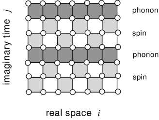
Figure 1: The schematic representation of the ($1+1$)-dimensional lattice of $N=6$ and $M=2$.

We use a quantum Monte Carlo method in order to investigate thermodynamic properties. We adopt the recipe introduced by Hirsch to deal with the spin-phonon coupled system. [20, 21] The partition function is expressed in the path-integral formula including both spin and lattice degrees of freedom,

$$Z={\rm Tr}_{\rm spin}\left(\prod_{i,j}\int{\rm d}u_{i,j}\right)\prod_{j=1}^{M}$$

$$\times\exp\left[-\Delta\tau\sum_{i={\rm odd}}J\left[1+\alpha(u_{i,j}-u_{i+1,j})\right]\mbox{\boldmath$S$}_{i,j}\cdot\mbox{\boldmath$S$}_{i+1,j}\right]$$

$$\times\exp\left[-\Delta\tau\sum_{i={\rm even}}J\left[1+\alpha(u_{i,j}-u_{i+1,j})\right]\mbox{\boldmath$S$}_{i,j}\cdot\mbox{\boldmath$S$}_{i+1,j}\right]$$

$$\times\exp\left[-\Delta\tau\sum_{i=1}^{N}\left[\frac{m}{2}\left(\frac{u_{i,j+1}-u_{i,j}}{\Delta\tau}\right)^{2}\right.\right.$$

$$\hskip 56.9055pt\left.\left.+\frac{k}{2}(u_{i,j}-u_{i+1,j})^{2}\right]\right],$$ (2)

where $M$ is the Trotter number and $\Delta\tau=\beta/M$ with the inverse temperature $\beta$. In Fig. 1 we show an example of the transformed ($1+1$)-dimensional lattice. There are three layers in a unit for the imaginary-time axis, namely, two checkerboard layers for the spin-spin part and one layer for the phonon part. The unit of layers is heaped in $M$ layers.

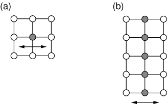
Figure 2: The schematic representation of the change of the lattice configuration. (a) the local flip and (b) the global flip in which the lattice points denoted by solid circles are flipped together.

We perform Monte Carlo simulations in the ($1+1$)-dimensional classical system. The spin configuration is updated by the loop algorithm [17, 18] with the fixed lattice configuration. The loop algorithm is powerful to calculate physical quantities at considerable low temperature. Therefore it is useful to observe the spin-Peierls correlation at low temperature. In the loop algorithm, a graph element is assigned to each plaquette with a probability which depends on the value of the exchange coupling on the plaquette. In the present case, the value of the exchange coupling varies along the imaginary-time axis due to quantum lattice fluctuation. Hence we can not take the limit of continuous imaginary time. [19] In this study, the lattice configuration is updated by the Metropolis algorithm with the fixed spin configuration. We perform a local flip and a global flip for the update of the lattice as shown in Fig. 2. The local flip updates the lattice state at a point in the ($1+1$)-dimensional space, which causes a curved world line of the lattice configuration. For convenience of the calculation, the change of the lattice displacement is discretized by a small value $u_{\rm unit}$. First, whether the lattice point moves right or left is chosen with a probability $1/2$. Next, whether the move takes place or not is chosen according to the Boltzmann weight. The local flip is efficient for the case where quantum lattice fluctuation is large. When quantum lattice fluctuation is small and the lattice tends to move adiabatically, we adopt the global flip of the lattice state. The global flip updates the lattice states by a parallel shift of all the points in a world line. We perform the spin update and the lattice update alternately. Therefore we obtain the thermal distribution of both spin and lattice degrees of freedom. Typically, the initial $10^{5}$ Monte Carlo steps (MCS) are discarded for thermalization, and the following $10^{6}$ MCS are used to calculate physical quantities. The sampled data is divided into 10 bins, and the errorbar is estimated from the standard deviation for the data set of these 10 bins.

For the simplicity of the notation, we use the bond distortion,

$$\Delta_{i}=\alpha(u_{i}-u_{i+1}),$$ (3)

as a variable instead of the lattice displacement $u_{i}$ itself. We provide a cutoff for the bond distortion $|\Delta_{i}|\leqslant\Delta_{\rm cutoff}=0.6$, i.e., $0.4\leqslant J_{i}\leqslant 1.6$, to confine the exchange coupling to be antiferromagnetic. As we have pointed out, [6] the variation of the bond is very large at finite temperature if we use the Hamiltonian of eq. (1). Such large deviation is not realistic and we need some nonlinear suppression of the bond deviation. The cutoff plays the role of this suppression.

3 Lattice Configuration

The bond configuration characterizes the spin-Peierls state, because the bond takes either a uniform configuration in the uniform state or an alternating configuration in the spin-Peierls state. We investigate the effect of both thermal fluctuation and quantum fluctuation on the bond configuration.

Figure 3: The bond correlation function along the real-space axis for (a) $m=10000$, (b) $m=100$ and (c) $m=1$. The left figures are the data at $T=0.5$ for the system of $N=64$ and $M=12$. The right figures are the data at $T=0.02$ for the system of $N=64$ and $M=384$.

In Figs. 3 we show the bond correlation function from the left edge bond,

$$C_{\rm bond}(1,j)=\langle\Delta_{1}\Delta_{j}\rangle,$$ (4)

where $\langle\cdots\rangle$ denotes the thermal average. For a heavy mass $m=10000$, the bond correlation function depicted in Fig. 3(a) agrees with our previous results without quantum fluctuation of the bond. [6] At a high temperature $T=0.5$, each bond fluctuates with no correlation and the bond takes a uniform configuration on the thermal average due to thermal fluctuation of the bond. At a very low temperature $T=0.02$, the bond alternation occurs with strong correlation extending over the chain. When the mass decreases, the effect of quantum lattice fluctuation becomes remarkable. As we show in Figs. 3(b) and 3(c), the alternating structure at low temperature disappears. We find no alternating pattern for a light mass $m=1$, where the bond takes a uniform configuration because the bond alternation is disarranged by quantum fluctuation of the bond.

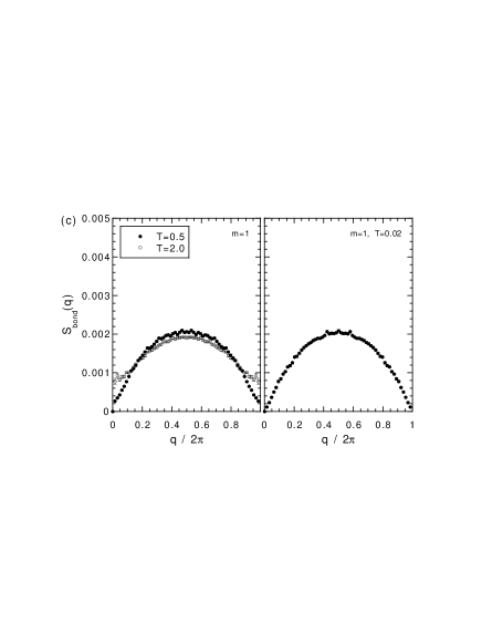
Figure 4: The bond structure factor for (a) $m=10000$, (b) $m=100$ and (c) $m=1$. The left figures are the data at $T=0.5$ for the system of $N=64$ and $M=12$. The right figures are the data at $T=0.02$ for the system of $N=64$ and $M=384$. The open circle in (c) denotes the data at $T=2.0$ for the system of $N=64$ and $M=4$.

Thus the uniform bond configuration is realized due to thermal fluctuation at high temperature and due to quantum fluctuation at low temperature. The shape of the bond correlation function is simply flat for both cases. Therefore the bond correlation function is insufficient to characterize the difference of the nature of the bond fluctuation in both cases. For the purpose of clarifying the distinction between the classical bond fluctuation and the quantum one, we investigate the bond structure factor,

$$S_{\rm bond}(q)=\langle|\Delta_{q}|^{2}\rangle,$$ (5)

where

$$\Delta_{q}=\frac{1}{N}\sum_{j=1}^{N}\Delta_{j}{\rm e}^{{\rm i}qj}.$$ (6)

In Fig. 4(a) we show the bond structure factor for $m=10000$. At $T=0.5$, $S_{\rm bond}$ is flat as a result of the mixture of various modes of the motion, which means that each bond fluctuates independently. At $T=0.02$, the lattice forms the bond-alternate structure and $S_{\rm bond}$ has a Bragg peak at $q=\pi$. Except for $q=\pi$, $S_{\rm bond}$ is very small and the fluctuation is independent of the position of the bond. These structures are consistent with the results of the classical lattice system.

On the other hand, when the mass decreases, the bond structure factor shows characteristic dependence on the temperature. In Fig. 4(b) we show the bond structure factor for $m=100$. $S_{\rm bond}$ remains flat at $T=0.5$. At $T=0.02$, comparing with the data for $m=10000$, the amplitude of the Bragg peak becomes small and the fluctuation of various modes grows in addition to $q=\pi$. This structure factor with the mixture of various modes corresponds to the correlation function shown in the right of Fig. 3(b), where the alternate structure is hardly detected.

When the mass decreases furthermore, $m=1$, $S_{\rm bond}$ has a sinusoidal shape at both $T=0.5$ and $T=0.02$ as shown in Fig. 4(c). The sinusoidal structure factor is interpreted as follows. For light mass, the second term of eq. (1) is much larger than the first one. Namely, the lattice moves almost independently of the spin configuration. Therefore, in the following, we investigate the lattice part of eq. (1),

$$H_{\rm phonon}=\sum_{j=1}^{N}\left[\frac{1}{2m}p_{j}^{2}+\frac{k}{2}(u_{j}-u_{j+1})^{2}\right].$$ (7)

The operators of the lattice displacement $u_{j}$ and the momentum $p_{j}$ are expressed by the creation operator $a_{q}^{{\dagger}}$ and the annihilation operator $a_{q}$ of the phonon,

$$u_{j} = \sum_{q}\sqrt{\frac{1}{2Nm\omega_{q}}}(a_{-q}^{{\dagger}}+a_{q}){\rm e}^{{\rm i}qj},$$ (8)

$$p_{j} = \sum_{q}{\rm i}\sqrt{\frac{m\omega_{q}}{2N}}(a_{-q}^{{\dagger}}-a_{q}){\rm e}^{{\rm i}qj},$$ (9)

where

$$\omega_{q}^{2}=4\omega^{2}\sin^{2}\frac{q}{2}.$$ (10)

Then eq. (7) is transformed into

$$H_{\rm phonon}=\sum_{q}\omega_{q}\left(a^{{\dagger}}_{q}a_{q}+\frac{1}{2}\right).$$ (11)

The Fourier component of the bond distortion is expressed by

$$\Delta_{q}=2{\rm i}\alpha\sqrt{\frac{1}{2Nm\omega_{q}}}(a_{q}^{{\dagger}}+a_{-q}){\rm e}^{-{\rm i}q/2}\sin\frac{q}{2}.$$ (12)

At $T=0$, all the nomal modes are in the ground state, i.e., $a_{q}|0\rangle=0$, and $S_{\rm bond}$ is given by

$$S_{\rm bond}(q) = \langle|\Delta_{q}|^{2}\rangle$$ (13)

$$= \frac{2\alpha^{2}}{Nm\omega_{q}}\sin^{2}\frac{q}{2}\langle 0|(a_{-q}^{{\dagger}}+a_{q})(a_{q}^{{\dagger}}+a_{-q})|0\rangle$$

$$= \frac{\alpha^{2}}{Nm\omega}\sin\frac{q}{2}.$$

Namely, the zero-point motion gives the sinusoidal structure factor. This result agrees with the sinusoidal shape of our Monte Carlo results. But we find that the amplitude in Fig. 4(c) ($\cong 0.0021$) is smaller than that of eq. (13) ($\cong 0.0156$). This discrepancy is caused by the cutoff for the bond distortion. The bond distortion is suppressed due to the cutoff and the structure factor becomes small. In Monte Carlo simulations of the lattice part without the spin part, it is confirmed that the amplitude agrees with that of eq. (13) in the case where the cutoff is large enough, and the amplitude agrees with that of Fig. 4(c) in the case where the cutoff is the same as that we provide in the spin-Peierls model. Thus we conclude that the lattice fluctuation for light mass is characterized by the zero-point quantum fluctuation of the lattice. It should be mentioned that when the temperature is larger than $\omega=\sqrt{k/m}$, $S_{\rm bond}$ is influenced by the excited state of the phonon. In the present case, we actually find that $S_{\rm bond}$ is influenced by excited states at $T=2.0$ ($>\omega=1.0$) and changes from the sinusoidal shape to a flat shape as shown by the open circle in the left of Fig. 4(c).

4 Quantum Lattice Fluctuation

In the thermal average, the lattice takes either the uniform configuration for light mass or the dimerized configuration for heavy mass due to the spin-phonon coupling. On the other hand, in a snapshot in the Monte Carlo simulation, the world line of the lattice shows various configurations due to quantum lattice fluctuation. For heavy mass, the motion of the lattice is regarded to be adiabatic and the world-line configuration of the lattice is straight along the imaginary-time axis. The straight world line parallels with each other and forms the dimerized configuration. As the mass decreases, quantum lattice fluctuation becomes relevant and the world line of the lattice begins to fluctuate along the imaginary-time axis. The deviation of the world line may suppress the bond-alternating order. Here we introduce the order parameter for the bond-alternating order,

$$\Delta_{\rm sg}^{2}=\left\langle\left(\frac{1}{N}\sum_{i=1}^{N}(-1)^{i}\Delta_{i}\right)^{2}\right\rangle.$$ (14)

In addition, we explore how the bond alternation is disarranged due to quantum lattice fluctuation by investigating the following quantity,

$$\Delta_{\rm sgt}^{2}=\left\langle\left(\frac{1}{\beta}\int_{0}^{\beta}{\rm d}\tau\frac{1}{N}\sum_{i=1}^{N}(-1)^{i}\,{\rm e}^{H\tau}\Delta_{i}\,{\rm e}^{-H\tau}\right)^{2}\right\rangle,$$ (15)

where ${\rm e}^{H\tau}\Delta_{i}\,{\rm e}^{-H\tau}$ represents the value of $\Delta_{i}$ at the imaginary time $\tau$. In Figs. 5 we show the size dependence of $\Delta_{\rm sg}^{2}$ and $\Delta_{\rm sgt}^{2}$ at $T=0.02$. For $m=10000$, $\Delta_{\rm sg}^{2}$ agrees with $\Delta_{\rm sgt}^{2}$, which indicates that the bond-alternating order develops in both the real-space axis and the imaginary-time axis. In fact, there the world line is straight along the imaginary-time axis. When the mass decreases, the absolute values of the bond-alternating correlations decrease as shown in Figs. 5(b) and 5(c). In particular, $\Delta_{\rm sgt}^{2}$ is much reduced comparing with $\Delta_{\rm sg}^{2}$ for finite size systems. This is due to the deviation of the world-line configuration along the imaginary-time axis. For $m=100$, however, we find that $\Delta_{\rm sg}^{2}$ and $\Delta_{\rm sgt}^{2}$ converge to almost the same finite value in the thermodynamic limit. The amount of the bond alternation for $m=100$ is smaller than that for $m=10000$. For $m=1$, the bond configuration is uniform on the thermal average in the thermodynamic limit. There $\Delta_{\rm sg}^{2}$ shows $1/N$ dependence which indicates a short range order of the bond alternation, while $\Delta_{\rm sgt}^{2}$ is almost zero because the correlation length along the imaginary-time axis is much shorter than $\beta$ as we will see in §6.

Figure 5: The size dependence of the order parameters for the bond alternation $\Delta_{\rm sg}^{2}$ (solid circle) and $\Delta_{\rm sgt}^{2}$ (open circle) for (a) $m=10000$, (b) $m=100$ and (c) $m=1$ at $T=0.02$. $M=384$.

5 Mass Dependence of Magnetic Properties

The spin-phonon coupling causes deviation of magnetic properties from those of the uniform lattice system. First we consider the effect of thermal fluctuation of the lattice at high temperature where the spin-Peierls correlation is not relevant. In Fig. 6 we show the temperature dependence of the magnetic susceptibility for a high temperature region. We have calculated for the adiabatic lattice system. [6] For comparison, the data for the adiabatic lattice system (dotted line) and the uniform lattice system (solid line) are shown in the figure. For $m=10000$, the magnetic susceptibility agrees with that of the adiabatic lattice system. As has been pointed out in numerical works, [12, 14, 6] the magnetic susceptibility deviates from that of the uniform lattice system even at high temperatures due to thermal fluctuation of the lattice. As the mass decreases, the magnetic susceptibility approaches that of the uniform lattice system monotonously. For $m=1$, the magnetic susceptibility agrees with that of the uniform lattice system well, even though the lattice strongly fluctuates. This fact has been seen in previous works for models with the second quantization of the lattice. [12, 14]

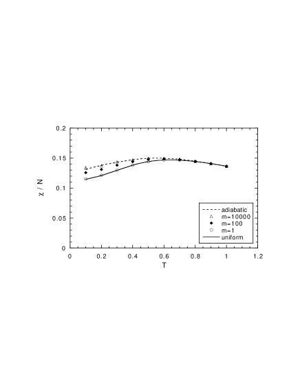
Figure 6: The temperature dependence of the magnetic susceptibility. The data are calculated for the system of $N=64$ and extrapolated with respect to the Trotter number. The dotted line denotes the data for the adiabatic lattice system of $N=64$ and the solid line denotes the data for the uniform lattice system of $N=64$.

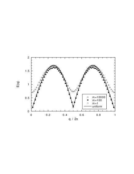
Figure 7: The magnetic elementary excitation spectrum in the ground state. The data are calculated at $T=0.02$ for the system of $N=64$ and $M=384$. The solid line denotes the data for the uniform lattice system of $N=64$.

Now we consider the effect of quantum fluctuation of the lattice at low temperature. In order to grasp the magnetic behavior from a microscopic point of view, we investigate the magnetic excitation spectrum. It can be extracted from the imaginary-time correlation function of the spin, [22, 23]

$$S_{\rm spin}(q,\tau)=\langle{\rm e}^{H\tau}S_{q}^{z}{\rm e}^{-H\tau}S_{-q}^{z}\rangle,$$ (16)

where

$$S_{q}^{z}=\frac{1}{N}\sum_{j=1}^{N}S_{j}^{z}{\rm e}^{{\rm i}qj}.$$ (17)

The dispersion relation $E(q)$ of the elementary excitation is obtained by

$$E(q)=-\frac{\partial}{\partial\tau}\ln[S_{\rm spin}(q,\tau)]$$ (18)

for large $\tau$. In Fig. 7 we show the magnetic elementary excitation spectrum at $T=0.02$ for several values of the mass. The solid line denotes the data for the uniform lattice system of $N=64$, where we find a small energy gap due to the finite size effect. For $m=10000$, the lattice motion is adiabatic and the bond alternation occurs at low temperature. Accordingly, we find an energy gap at $q=\pi$ clearly. On the other hand, we find that the energy gap becomes small drastically as the mass decreases. For $m=1$, $E(q)$ coincides with that of the uniform lattice system. Thus we find that not only the magnetic susceptibility but also the microscopic magnetic characteristic agrees with those of the uniform lattice system. Therefore we conclude that this agreement is intrinsic. In the next section, we study the physical background of this agreement.

6 Quantum Narrowing Effect

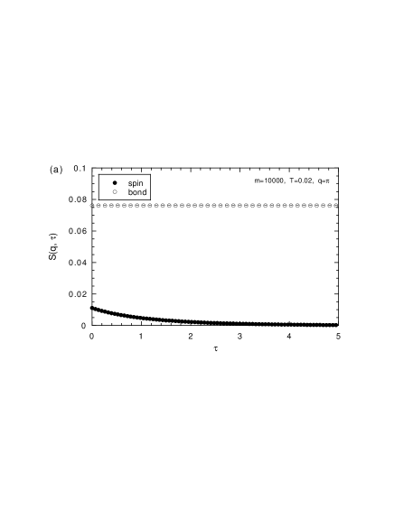
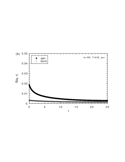
Figure 8: The imaginary-time correlation functions of the spin and the bond for $q=\pi$ at $T=0.02$. (a) $m=10000$, (b) $m=100$ and (c) $m=1$. The solid circle and the open circle denote the data in terms of the spin and the bond, respectively. The data are calculated for the system of $N=64$ and $M=384$.

In this section we consider the reason why the expectation value of magnetic properties of the light mass system coincides with that of the uniform lattice system. As we mentioned above, the motion of the lattice is almost independent of the spin configuration because the mass is light. On the other hand, the motion of the spin may be affected by the bond fluctuation. Generally speaking, however, the effect of fast fluctuation is to be neglected, which is known as the motional narrowing effect. Namely, when the fluctuation is much fast compared to the time scale which we would like to observe, the fluctuation is leveled off and does not affect other degrees of freedom. In the present case, what comes into question is the degree of quantum fluctuations of the spin and the lattice. The correlation along the imaginary-time axis gives information on the time scale of quantum fluctuation. We investigate $S_{\rm spin}(q,\tau)$ defined in eq. (16) and the imaginary-time correlation function of the bond,

$$S_{\rm bond}(q,\tau)=\langle{\rm e}^{H\tau}\Delta_{q}{\rm e}^{-H\tau}\Delta_{-q}\rangle.$$ (19)

In Figs. 8 we compare both imaginary-time correlation functions for $q=\pi$ at $T=0.02$. For $m=10000$, $S_{\rm spin}(q,\tau)$ decays along the imaginary-time axis quickly and $S_{\rm bond}(q,\tau)$ keeps a constant value. The spin fluctuation is much faster than the bond fluctuation. Namely, the time scale of the spin fluctuation $\tau_{\rm spin}$ is much smaller than that of the bond fluctuation $\tau_{\rm bond}$ ($\tau_{\rm spin}\ll\tau_{\rm bond}$). In this case, the lattice vibration can be regarded to be adiabatic. On the other hand, as the mass decreases, the inequality relation between the two time scales is reversed. For $m=1$, $S_{\rm bond}(q,\tau)$ decays quite rapidly. This value of $\tau_{\rm bond}$ is much shorter than $\beta=(0.02)^{-1}=50$ as we expected by the observation of $\Delta_{\rm sgt}^{2}$ in §4. Here the relaxation of $S_{\rm bond}(q,\tau)$ is much faster than that of $S_{\rm spin}(q,\tau)$, i.e., $\tau_{\rm spin}\gg\tau_{\rm bond}$. This means that the lattice fluctuates much faster than the time scale of the motion of the spin. Thus we conclude that a sort of narrowing effect happens and the lattice is effectively fixed to be uniform. We call this phenomenon “quantum narrowing effect”.

7 Summary and Discussion

In this paper we investigated a one-dimensional $S=1/2$ antiferromagnetic Heisenberg model coupled to quantum lattice vibration using a quantum Monte Carlo method. We studied the mass dependence of various physical quantities. For heavy mass, quantum lattice vibration is regarded as the adiabatic motion and the system dimerizes at low temperature. When the mass decreases, the bond-alternate correlation is reduced due to the deviation of the world-line configuration of the lattice. For light mass, the spin-Peierls correlation does not grow even at low temperature, and the ground-state lattice fluctuation is equivalent to the zero-point vibration of the phonon. The lattice fluctuation does not affect the magnetic behavior. We found the separation of time scales of quantum fluctuations of spin ($\tau_{\rm spin}$) and lattice ($\tau_{\rm bond}$) degrees of freedom. The time scales change with the mass. The motion of the lattice can be regarded to be adiabatic for heavy mass, where $\tau_{\rm spin}\ll\tau_{\rm bond}$. On the other hand, the motion of the lattice is smeared out due to the narrowing effect for light mass, where $\tau_{\rm spin}\gg\tau_{\rm bond}$.

For intermediate mass, $m=100$ [Fig. 8(b)], imaginary-time correlation functions of the spin and the bond decay with almost the same decay time. In such cases we expect that the spin fluctuation and the bond fluctuation resonate with each other. The resonance of quantum fluctuations would cause a multiple quantum state of spin and lattice degrees of freedom, which is an interesting problem in the future.

References

- [1] J. W. Bray, L. V. Interrante, I. S. Jacobs and J. C. Bonner: in Extended Linear Chain Compounds, ed. J. S. Miller (Plenum Press, New York and London, 1983) Vol.3.
- [2] J. W. Bray, H. R. Hart, Jr., L. V. Interrante, I. S. Jacobs, J. S. Kasper, G. D. Watkins, S. H. Wee and J. C. Bonner: Phys. Rev. Lett. 35 (1975) 744.
- [3] M. Hase, I. Terasaki and K. Uchinokura: Phys. Rev. Lett. 70 (1993) 3651.
- [4] M. C. Cross and D. S. Fisher: Phys. Rev. B 19 (1979) 402.
- [5] T. Nakano and H. Fukuyama: J. Phys. Soc. Jpn. 49 (1980) 1679.
- [6] H. Onishi and S. Miyashita: J. Phys. Soc. Jpn. 69 (2000) 2634.
- [7] L. G. Caron and S. Moukouri: Phys. Rev. Lett. 76 (1996) 4050.
- [8] H. Zheng: Phys. Rev. B 56 (1997) 14 414.
- [9] G. S. Uhrig: Phys. Rev. B 57 (1998) R14 004.
- [10] G. Wellein, H. Fehske and A. P. Kampf: Phys. Rev. Lett. 81 (1998) 3956.
- [11] R. J. Bursill, R. H. McKenzie and C. J. Hamer: Phys. Rev. Lett. 83 (1999) 408.
- [12] A. W. Sandvik, R. R. P. Singh and D. K. Campbell: Phys. Rev. B 56 (1997) 14 510.
- [13] A. W. Sandvik and D. K. Campbell: Phys. Rev. Lett. 83 (1999) 195.
- [14] R. W. Kühne and U. Löw: Phys. Rev. B 60 (1999) 12 125.
- [15] A. Weiße, G. Wellein and H. Fehske: Phys. Rev. B 60 (1999) 6566.
- [16] M. Holicki, H. Fehske and R. Werner: Phys. Rev. B 63 (2001) 174417.
- [17] N. Kawashima and J. E. Gubernatis: J. Stat. Phys. 90 (1995) 169.
- [18] H. G. Evertz: cond-mat/9707221.
- [19] B. B. Beard and U.-J. Wiese: Phys. Rev. Lett. 77 (1996) 5130.
- [20] J. E. Hirsch, D. J. Scalapino, R. L. Sugar and R. Blankenbecler: Phys. Rev. Lett. 47 (1981) 1628.
- [21] E. Fradkin and J. E. Hirsch: Phys. Rev. B 27 (1983) 1680.
- [22] S. Yamamoto and S. Miyashita: J. Phys. Soc. Jpn. 63 (1994) 2866.
- [23] S. Yamamoto: Phys. Rev. B 51 (1995) 16 128.