Effects of stochastic nucleation in the first order phase transition

In the system during the first order phase transition new supercritical formations of a new phase appear with some fixed probability, but appear in stochastic manner. In a system with macroscopic sizes due to a giant value of the Avogadro number there appears rather big number of droplets. It allows to use the averaged characteristics to construct kinetics of a nucleation process. Kinetics based on averaged characteristics is described in [6]. In this paper the time evolution is constructed and it is possible to extract elementary intervals where thermodynamic parameters and the nucleation rate have small variations. The total number of droplets is so big that at every elementary interval there appears a great number of droplets $\Delta N$. On the base of traditional thermodynamics one can state that the relative fluctuation $\delta\Delta N/\Delta N$ of droplets formed at elementary interval is small and has an order of $(\Delta N)^{1/2}$. This remark completely solves a problem of justification of nucleation description based on averaged characteristics. But recently there appears a set of papers [2], [1] where a stochastic effects (the effects of fluctuations of droplets formation) were described and investigated. Two approaches were formulated there. Authors didn’t hesitate that these approaches [1] , [2] gave different results. So, one has to analyze approaches [2], [1] and decide what is the true result.

An idea formulated in [1], [2], allows to establish corrections to the total number of droplets $N$ appeared in the system. It was supposed that these corrections are functions of $N$. To demonstrate the error of this approach it is sufficient to take two identical systems then to calculate them separately and to add results or to calculate correction directly for the total system. The results will differ.

One has to determine a real volume to which one has to refer the number of droplets. It is simple to do with the help of results from [8]. In that paper kinetics of nucleation for diffusion regime of droplets growth was constructed. It was shown that a solitary droplet perturbes vapor up to distances of an order $\sqrt{4Dt}$, where $D$ is diffusion coefficient, $t$ is a time from droplet formation. One can take as $t$ a time $t_{1}$ of nucleation period duration. A nucleation period is a period of intensive formation of droplets.

It allows to give a new definition of the volume $V_{1}$ where the number $N_{1}$ of droplets is formed. Namely this value has to be regarded as a volume of a system. This volume is $4\pi(4Dt_{1})^{3/2}/3$. If the sizes of the system are smaller than this value one has to take the volume of the system as this value. But such a small system can be hardly regarded as a macroscopic one. At least one has to analyze carefully the boundary conditions.

Naturally, the droplets appeared at different times perturbe initial phase at different distances. So, one can regard above formulas only as estimates. Some more rigorous equations can be found in [4].

The number of droplets $N_{1}$ isn’t too big as $N$ is. So, an analysis of stochastic effects has a real sense. It is interesting now to get all correction terms which are ascending with the number of droplets (but not only a leading term). To solve this task one has to modify approaches from [1], [2] where only a vague conclusion about the order of the leading term was made.

Complexity of this problem lies in conclusion that one can not directly use equations based on the theory with averaged characteristics. In [1], [2] some properties of solution on the base of averaged characteristics were starting points for constructions. This supposition was adopted without any justifications.

We shall consider the situation of decay. The new dimensionless parameter - the number of droplets destroys the universality observed in [6] for the theory based on averaged characteristics. Moreover, it is difficult even to formulate the system of equations. It radically complicates the problem.

The property of effective monodispersity formulated in [5] was used in [2] without any justifications. Generally speaking this property can not be directly used to calculate stochastic corrections. This leads to an error made in [2]. Now we shall formulate more correct approach.

Both approaches from [1] and [2] used the following property ”The droplets formed at the beginning of the nucleation period are the main consumers of vapor”. This property is valid, but it is substituted in [2], [1] by the following statement: ”The main source of stochastic effects are the free fluctuations of droplets formed at the beginning of the nucleation period. they govern the fluctuations of all other droplets”. But the last statement isn’t valid. So, one has to use some new methods which are presented below.

The use of monodisperse approximation will lead to some errors. But due to universality of solution [6] these errors can not be be too big. Qualitatively everything is suitable, but precision will be very low.

The same conclusion will be valid for calculations based on some model behavior of supersaturation (justification is valid for a vapor consumption, but not for stochastic effects). Here the final result will be more precise but it comes from rather spontaneous artificial choice of some parameter which equals in [1] to $1/2$. In [1] it is supposed that until some moment (it is chosen in [1] as a half of nucleation period) the droplets are formed under ideal conditions and namely these droplets determine a vapor consumption. This approach taken from [3], was used in [1] in slightly another sense. It is supposed that droplets formed during a first half of nucleation period are the main source of stochastic effects. The last statement was not justified in [1] and it is rather approximate. The relative correctness of a result was attained due to specific compensation of different errors of approximations used in [1].

All arguments listed above lead to necessity of reconsideration which will be made in this publication. A plan will be the following

• On the basis of algebraic approach we shall see that stochastic effects are small

• A smallness of stochastic effects allows to seek the solution on the base of the theory with averaged characteristics. But we have to take stochastic effects from all droplets formed during the nucleation period.

• The possibility to take into account the role of all droplets can be ensured by the property of similarity of nucleation conditions during the nucleation period. This property can be considered in two senses - 1) in the local differential sense and 2) in the integral sense in frames of the first iteration. The local property will be used in justification of the smallness of stochastic effects and the integral property will be used to calculate the stochastic corrections.

All analytical results will be checked by computer simulation and a coincidence will be shown

All mentioned constructions will be valid for an arbitrary first order phase transition.

The law of droplets growth will be a free molecular one, the linear size grows with velocity independent from its value. Consideration of other regimes can be attained in frames of the current approach by some trivial substitutions, but one has to take into account that the new regime requires new approaches to construct nucleation kinetics as it is shown in [8]. So, we can not agree with he statement in [2] that one of results is an account of stochastic effects in a diffusion regime of droplets growth. This effect has to be taken into account by application of methods presented in [7].

Dynamic conditions can be easily considered by direct generalization of methods presented here and we needn’t to present it in details.

1 Estimates for stochastic effects

We consider the theory based on averaged characteristics. It is supposed to be known [6], that the supersaturation $\zeta$ behavior can be determined after certain renormalizations by the following equation

$$\psi(z)=\int_{0}^{t}dx(z-x)^{3}\exp(-\psi)$$

A good approximation for solution and for a distribution $\exp(\psi)$ over linear sizes is $f_{1}=\exp(-z^{4}/4)$. The form of $f_{1}$ is given by fig.1

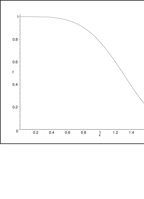
Figure 1: A form of approximation for size spectrum

It is seen that at $z_{0}=1.25$ the nucleation period stops.

This approximation has rather high precision [5]. It is based on the following law of substance accumulation

$$G=z^{4}/4=\int_{0}^{z}(z-x)^{3}\equiv\int_{0}^{z}g,\ \ g=(z-x)^{3}$$

For any moment $t$ or $z$ a function $g$ has one and the same form. This is a similarity of nucleation conditions. We see that every time the droplets formed at the last third of a period from beginning of nucleation until a current moment will accumulate a negligible quantity of substance. The relative quantity of the substance there has an order of ($\sim 1/27$) and is so small that even if there will be fluctuations the quantity will be small.

From the form of $f_{1}$ it is seen that until $z_{=}\equiv 0.7z_{0}$ all droplets will deplete vapor rather weak. It will be important for future analysis.

The mentioned property of $g$ allows to use a monodisperse approximation [5] not only at the end of nucleation but in every moment of the nucleation period [5]. Let $t(G)$ be the moment when there are $G$ molecules in droplets (in appropriate units). An application of the monodisperse approximation [5] leads to

$$\frac{1}{4}N(z)z^{3}=G$$

Now it will be possible to repeat all constructions [2] with $G$ instead of $1$ (in renormalized units, before renormalization it would be $1/\Gamma$ (see [6]). The sense of these transformations is rather evident. Let $t(z)$ be the current moment of time ($z$ is the coordinate of ta spectrum front, actually $t$ is proportional $z$). We suppose that before $az$ ($a$ is some parameter) droplets are formed without mutual influence and one can write Poisson’s distribution. Then a natural restriction on $a$ appeared, namely $a<0.7*z_{0}/z$. Then we suppose that the influence of other droplets on its own formation is negligible (this follows from $2*0.7=1.4>1.25$ and from notation about the last third of nucleation period). Then it is possible to write Poisson’s distribution for the second group of droplets, but with parameters depended on stochastic values - characteristics of the droplets distribution from the first group. Rigorously speaking one has to use the first four moments of the droplets distribution in accordance with [6], but for simplicity we shall use here only the zero momentum. As a compensation for this simplicity we has to use here $a=0.25$.

Then one has to come from Poisson’s distributions to Gauss distributions and integrate them with account of connection between stochastic parameters of embryos formation from the first group and parameters of distribution from the second group. Unfortunately, in [2] the final result was an expression for distribution, but not for the number of droplets which can be observed in experiment. Beside this the expression for the distribution was calculated only in a leading term which is certainly a Gauss distribution. Corrections haven’t been established.

Contrary to [2] we shall take into account all correction terms which comes from transition from Poisson’s distributions to Gauss distributions and corrections for nonlinear connection between group distributions. We shall take all terms which are growing when the total number of droplets grows. We shall get the following result for droplets distribution

$$P=(\frac{9a}{2\pi N(3a+1)})^{1/2}\exp(-\frac{9a}{3a+1}\frac{D_{s}^{2}}{2})(1+y)$$

where

$$D_{s}=\frac{\hat{N}-N}{\sqrt{N}}$$

$\hat{N}$ - some stochastic value of the total number of droplets, $N$ - the mean value of droplets and $y$ is the correction for spectrum.

At $=1/4$ we get

$$y=\frac{1}{74088}D_{s}(8087D_{s}^{2}-10269)s+(-\frac{4}{9}+\frac{305}{1176}D_{s}^{2}$$

$$-\frac{8503}{1176}D_{s}^{2}-\frac{85903}{12446784}D_{s}^{4}+\frac{65399569}{10978063488}D_{s}^{6})s^{2}$$

where

$$s\equiv\sqrt{N}$$

is a small parameter of decomposition. To get all ascending corrections we must fulfill decomposition until $s^{2}$. At arbitrary $a$ we get the following expression

$$1+w_{1}s+w_{2}s^{2}$$

Here

$$w_{1}=-\frac{1}{6}((486l^{2}+486D_{s}^{2}l^{12}-972l^{11}D_{s}^{2}+324l^{4}-648D_{s}^{2}l^{10}+756l^{9}$$

$$+810l^{9}D_{s}^{2}-459l^{8}+297D_{s}^{2}l^{8}-135l^{7}D_{s}^{2}-$$

$$387l^{7}+90l^{6}D_{s}^{2}-153l^{6}+27l^{5}D_{s}^{2}-213l^{5}-66l^{4}D_{s}^{2}-3l^{4}+27l^{3}-3l^{3}D_{s}^{2}+16l^{2}D_{s}^{2}-3l^{2}+$$

$$9l+lD_{s}^{2}+D_{s}^{2})D_{s})/((1+3l^{2})^{3}(l+1)(-1+l^{2}))$$

where

$$l=\sqrt{a}$$

and

$$w_{2}=w_{02}/((l+1)^{2}(-1+l^{2})(1+3l^{2})^{6}l^{2})$$

$$w_{02}=\sum_{i=0}^{3}q_{2i}D_{s}^{2i}$$

$$q_{0}=-\frac{1}{12}-\frac{1}{6}l+\frac{243}{4}l^{16}-\frac{135}{2}l^{7}-90l^{8}-\frac{87}{2}l^{6}+\frac{243}{2}l^{14}+\frac{81}{2}l^{12}$$

$$-\frac{153}{2}l^{10}-\frac{67}{6}l^{4}-\frac{225}{2}l^{9}-\frac{3}{2}l^{2}-\frac{81}{2}l^{11}+\frac{243}{2}l^{13}-\frac{243}{2}l^{15}-\frac{17}{6}l^{3}$$

$$q_{2}=\frac{5265}{4}l^{12}+\frac{51}{2}l^{6}+117l^{10}+\frac{333}{2}l^{11}+\frac{31}{8}l^{4}$$

$$+\frac{17}{2}l^{5}+\frac{5049}{2}l^{14}-\frac{15309}{2}l^{19}+2079l^{13}$$

$$+31l^{8}-8748l^{18}+42l^{9}+\frac{24057}{2}l^{21}+\frac{103}{2}l^{7}+\frac{16767}{8}l^{20}+6561l^{22}$$

$$+\frac{4617}{2}l^{15}-3159l^{16}-8262l^{17}$$

$$q_{4}=-\frac{4413}{2}l^{13}-\frac{477}{2}l^{15}+7047l^{21}-\frac{1161}{4}l^{18}$$

$$+\frac{361}{6}l^{8}+\frac{105}{2}l^{11}-\frac{104247}{4}l^{22}-\frac{3}{4}l^{4}+17091l^{20}$$

$$-5103l^{23}+\frac{43}{6}l^{5}-\frac{31185}{4}l^{19}+7965l^{17}-\frac{3213}{4}l^{12}-\frac{475}{3}l^{10}+510l^{14}-\frac{49}{6}l^{7}+\frac{23}{4}l^{6}$$

$$+\frac{1}{12}l^{3}+{44469}{4}l^{24}-\frac{1}{12}l^{2}-\frac{6903}{4}l^{16}+\frac{74}{3}l^{9}$$

$$q_{6}=-13122l^{25}-\frac{40419}{8}l^{18}+\frac{17253}{2}l^{20}-\frac{24057}{2}l^{22}+4374l^{24}+\frac{6561}{2}l^{26}-$$

$$\frac{48843}{2}l^{21}-\frac{623}{24}l^{8}+\frac{59}{36}l^{6}-\frac{3609}{4}l^{14}$$

$$-\frac{57}{8}l^{12}+\frac{411}{4}l^{10}+\frac{11}{24}l^{4}+\frac{1}{72}l^{2}-\frac{29}{12}l^{7}-\frac{345}{4}l^{11}+\frac{1}{36}l^{3}+$$

$$\frac{13}{36}l^{5}+\frac{65}{4}l^{9}+\frac{2421}{4}l^{13}-\frac{7857}{4}l^{15}+$$

$$\frac{8667}{4}l^{17}+28431l^{23}+7047l^{19}+\frac{24705}{8}l^{16}$$

Having integrated this expression we get corrections to droplets number. The term at $s$ gives zero after integration and the first correction has an order of $\sim s^{2}$ and doesn’t depend on the total number of droplets. A coefficient at $s^{2}$ has at $a=1/4$ a value

$$d_{0}=311/3024$$

At arbitrary $a$ a coefficient at $s^{2}$ in correction for the total number of droplets will be

$$d_{a}=\frac{1}{72}[108a^{6}+540a^{11/2}-72a^{5}-930a^{9/2}-336a^{4}+$$

$$713a^{7/2}+158a^{3}+4a^{2}-203a^{5/2}-6a+39a^{3/2}-3a^{1/2}]/[a^{3/2}(1-a)^{2}(1+3a)]$$

It will be interesting to compare results with and without corrections from transition from Poisson’s distribution to Gauss distribution. At the leading term there will be no change. At correction terms we have

$$y=\frac{17}{74088}D_{s}(-2331+289D_{s}^{2})s+(\frac{17}{196}D_{s}^{2}+$$

$$\frac{732037}{12446784}D_{s}^{4}+\frac{24137569}{10978063488}D_{s}^{6}-\frac{13}{36})s^{2}$$

$$d_{0}=-37/126$$

$$d_{a}=\frac{1}{72}(648a^{11/2}-216a^{5}-1062a^{9/2}+108a^{4}+753a^{7/2}-$$

$$30a^{3}-195a^{5/2}-12a^{2}+19a^{3/2}+6a-7a^{1/2})/(a^{3/2}(1+3a)(1-a)^{2})$$

It is seen that these corrections are small. At arbitrary $a$ except too small and $1$ (these values are unreal) we get values shown at fig.2

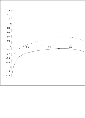
Figure 2: Dependence of corrections on $a$

Points show corrections with transition from Poisson’s distribution to Gauss distribution, a line shows corrections without transition from Poisson’s distribution to Gauss distribution. Both corrections have one and the same order and they are small.

One has to note that we have not take into account corrections from transition from summation to integration. It is made due to reasons formulated below. Really, we have at transition from summation in formula

$$P(N)=\sum_{\hat{N_{1}}}P_{1}(\hat{N_{1}},N_{1})P_{2}(N-\hat{N_{1}},N_{2}(N_{1}))$$

to integration

$$P(N)=\int d\hat{N_{1}}P_{1}(\hat{N_{1}},N_{1})P_{2}(N-\hat{N_{1}},N_{2}(N_{1}))$$

to use Euler’s decomposition. But discrete character in nucleation isn’t so trivial. The process of vapor consumption can not begin without the first droplet. The system will wait for droplet as long as it will be necessary. It shows that discrete effects are complicate and require a separate publication.

To use Poisson’s distribution for the first group one has to make the following notation. Really nucleation conditions for the first group don’t differ from the whole group. So, for distribution for the first group one has to take distribution $P_{1}$ with reduced halfwidth. But one can not attribute a halfwidth to Poisson’s distribution. That’s why we considered effects with and without corrections from transition from Poisson’s to Gauss distribution. So, we can use Gauss distributions as initial ones. For Gauss distribution one can easily reconsider the halfwidth. Then for $P_{1}$ one can take

$$P_{1}\sim\exp((\hat{N_{1}}-N_{1})^{2}/(2bN_{1}))$$

where $b$ is a renormalization coefficient. Distribution $P_{2}$ remains previous

$$P_{2}\sim\exp((\hat{N_{2}}-N_{2})^{2}/(2N_{2}))$$

where $N_{2}$ is given by

$$N_{2}=(1-\frac{1}{3}s+\frac{2}{9}s^{2}-\frac{14}{81}s^{3}+\frac{35}{243}s^{4}-\frac{91}{729}s^{5}-a)N$$

where $N$ is a mean total number of droplets,

$$s=\frac{\hat{N_{1}}-aN}{aN}$$

is a small parameter of an order $N^{-1/2}$

After integration one comes to

$$P\sim\exp(-\frac{9ab^{2}}{2(9a+b-6ba+9ba^{2}-9a^{2})}d^{2})$$

where

$$d=(\hat{N}-N)/\sqrt{N}$$

The halfwidth of the distribution $P_{1}$ must be equal to the halfwidth of $P$, which leads to

$$b=9\frac{a(1-a)}{-9a^{2}+15a-1}$$

Now we shall consider effects of renormalization. The ratio of corrections with renormalization and without renormalizations is given by

$$r=\frac{1}{9}\frac{\sqrt{-9a^{2}+15a-1}\sqrt{3a+1}}{a\sqrt{1-a}}$$

and it is shown at fig. 3

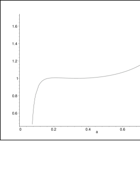
Figure 3: Ratio of halfwidths

For all reasonable values of $a$ it is approximately $1$. At $a=1/4$ we get $1.0041$ So, here the effect of similarity of nucleation conditions doesn’t lead to remarkable effects. It is only due to monodisperse approximation. Later this effect will be essential.

Instead of taking into account all moments of distribution we can directly calculate the effects on the base of explicit form of spectrum in frames of iteration procedure.

The result of this section is the following: we have proved that stochastic effects are small. Beside this we have demonstrated how to use the similarity of nucleation conditions. Here it is useless, but later this method will lead to some essential numerical results.

2 Stochastic effects in the iteration procedure

There is only one parameter which is essentially deviated by stochastic effects - it is dispersion of distribution or a halfwidth of distribution. Now we shall calculate this value.

The most advanced approach was suggested in [1]. But even this approach has many disadvantages.

We shall characterize a droplet by linear size $\rho$ which is the cubic root of its molecules number. Its velocity of growth does not depend on $\rho$.

Decomposition of a whole interval of nucleation into elementary intervals is connected with some difficulties. An elementary length $\tilde{\Delta}$ must satisfy according to [1] to two requirements: 1. A number of droplets formed during elementary length must be big. 2. An amplitude of a spectrum has to be approximately constant during an elementary interval.

It is clear that the second requirement can not be satisfied. Stochastic deviations of an amplitude leads to violation of the second requirement.

We shall apply the second requirement not to stochastic amplitude as it was stated in [1], but to averaged amplitude. Then the second requirement is : An averaged amplitude of a spectrum has to be approximately constant during an elementary interval.

Stochastic amplitudes $f_{i}$ are introduced in [1] as

$$f_{i}=\frac{N_{i}}{\tilde{\Delta}}$$

where $N_{i}$ is the number of droplets formed during $\tilde{\Delta}$. It isn’t stochastic value but partially averaged one. An expression for the number of molecules in droplets formed during interval number $i$ at a moment $t_{k}$ (it means that now we are at interval number $k$) will be the following one

$$\int_{x_{k-i}}^{x_{k-i+1}}f_{i}\rho^{3}d\rho=\frac{1}{4}f_{i}(x_{k-i+1}^{4}-x_{k-i}^{4})$$

The difference between forth powers corresponds to a constant amplitude of spectrum. It is wrong and then eq. (12) in [1] and all further equations are not correct.

But the is no necessity to use such a way to account the number of molecules in a new phase. It is absolutely sufficient to take the following expression

$$\int_{x_{k-i}}^{x_{k-i+1}}f_{i}\rho^{3}d\rho=N_{i}x_{k-i}^{3}$$

which is valid at $k-i\gg 1$. In a whole quantity of substance it is sufficient to take into account only droplets with $k-i\gg 1$. The relative weight of dismissed terms will be small.

Then for the total number of molecules in droplets at interval number $k$ we have the following expression

$$Q_{k}=\sum_{i=1}^{k}N_{i}x_{k-i}^{3}$$

where $x_{k-i}$ is appropriate coordinate or

$$Q_{k}\sim\sum_{i=1}^{k}N_{i}\hat{\Delta}^{3}(k-i)^{3}$$

This representation is important because now the note in [1] after eq. (15) isn’t necessary. This note stated that the probability for $N_{i}$ to deviate from $\bar{N}$ is very low. This note is doubtful because namely these deviations are the base for stochastic effects. Now there is no need in this note.

The next step is to build [1] two cycle construction for nucleation period. During the first cycle the main consumers of vapor appeared and during the second cycle they rule a process of formation of all other droplets. In [1] it is supposed that during the first cycle a vapor depletion is negligible and during the second cycle new droplets are absolutely governed by droplets from the first cycle. Now we shall analyze an effectiveness of such procedure.

We analyze an equation

$$\psi=\int_{0}^{z}(z-x)^{3}\exp(-\psi))dx$$

The first iteration [6] is practically precise solution and it gives the number of droplets

$$N_{tot}=\frac{1}{4}\frac{4^{1/4}\pi\sqrt{2}}{\Gamma(3/4)}=1.2818$$

A model solution requires that until $z=p$ there will be no depletion of vapor and then only droplets formed before $z=p$ will consume vapor. Then for a total number of droplets we have an expression

$$N_{tot\ appr}=p+\int_{p}^{\infty}\exp(-\frac{1}{4}x^{4}+\frac{1}{4}(x-p)^{4})dx$$

A ratio $N_{tot\ appr}/N_{tot}$ is given at fig. 4

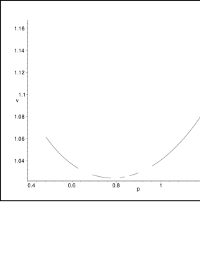
Figure 4: The ratio of mean numbers of droplets

Now it is clear that in [1] the value of parameter of separation into two cycles was not chosen in a good style (at least from the point of view in the theory with averaged numbers). We can also stress the smooth dependence $N_{tot\ appr}$ on $p$.

We shall study the probability $P_{k}$ of formation of stochastic number $N_{k}$ of droplets at the first $k$ elementary intervals [1].

Our constructions now resemble [1] but there is one essential difference. When we get a formula analogous to (30) [1] we have no necessity to linearize expression with respect to $(N_{i}-\bar{N_{i}})/\bar{N_{i}}$, where $N_{i}$ is a stochastic number of droplets formed at interval $i$, $\bar{N_{i}}$ is a mean number of droplets formed at interval $i$ (it is a function of stochastic numbers of droplets at preceding intervals). This linearization can not take place because a ratio $(N_{i}-\bar{N_{i}})/\bar{N_{i}}$ can be zero or can attain huge value (with low probability). It is more simple and more justified to linearize expression on $\sum_{i}\rho_{i}^{3}(N_{i}-\bar{N_{i}})/\bar{N_{i}}$ where $\rho_{i}$ is a linear size of droplets formed at interval $i$ (all of them have approximately the same size). Really, due to summation variations of $\sum_{i}\rho_{i}^{3}(N_{i}-\bar{N_{i}})/\bar{N_{i}}$ are much smaller than variations of $(N_{i}-\bar{N_{i}})/\bar{N_{i}}$.

Variations of $(N_{i}-\bar{N_{i}})/\bar{N_{i}}$ would be small only at very big numbers of droplets $N_{tot}$. One can get

$$(N_{i}-\bar{N_{i}})/\bar{N_{i}}\sim\bar{N_{i}}^{1/2}$$

$$N_{tot}\sim M\bar{N_{i}}$$

$M$ is a number of elementary intervals. So, the theory with linearization proposed in [1] would be well justified only in a region where the result can be obtained on the base of averaged characteristics. But the linearization proposed here leads to the same numerical expressions. For dispersion of the total distribution one can get

$$D^{\infty}=\tilde{N^{\infty}}(1-\frac{\beta}{\alpha})$$

where

$$\beta=\beta_{1}-\beta_{2}$$

$$\beta_{1}=8\int_{1/2}^{\infty}d\xi\int_{0}^{1/2}d\tau(\xi-\tau)^{3}\exp(-\xi^{4})$$

$$\beta_{2}=16\int_{1/2}^{\infty}d\xi\int_{1/2}^{\infty}d\eta\int_{0}^{1/2}d\tau(\tau-\xi)^{3}(\tau-\eta)^{3}\exp(-\xi^{4})\exp(-\eta^{4})$$

$$\alpha=\int_{0}^{\infty}dx\exp(-x^{4})$$

In two cycles construction the value of $\alpha$, which is proportional to the total number of droplets has to be reconsidered and recalculated on the base of two cycles. Then we have to use instead of previous $\alpha\equiv\alpha_{0}$ a new value

$$\alpha=\alpha_{1}\equiv 1/2+\int_{1/2}^{\infty}\exp(-x^{4}+(x-1/2)^{4})$$

We shall use parameter $p$ of separation of two cycles and we shall calculate $\alpha_{1}$ as

$$\alpha_{1}\equiv p+\int_{p}^{\infty}\exp(-x^{4}+(x-p)^{4})$$

Then according to fig. 4 we see that the ratio $\alpha_{0}/\alpha_{1}$ is greater than $1$ and $\alpha_{1}$ is greater than $\alpha_{0}$. Here we see that two-cycles construction is approximate one. Result for $D^{\infty}$ will differ from [1] and will be

$$D^{\infty}_{e}=\tilde{N^{\infty}}0.69$$

instead of

$$D^{\infty}_{f}=\tilde{N^{\infty}}0.67$$

as it is stated in [1]. The value $D_{e}^{\infty}$ differ from a real result more than one tenth. So, the new theory is necessary.

Now it is necessary to decide what $p$ shall we choose. At arbitrary $p$ the expression for $\beta$ will be the same but for $\beta_{1}$ $\beta_{2}$ we have

$$\beta_{1}=8\int_{p}^{\infty}d\xi\int_{0}^{p}d\tau(\xi-\tau)^{3}\exp(-\xi^{4})$$

$$\beta_{2}=16\int_{p}^{\infty}d\xi\int_{p}^{\infty}d\eta\int_{0}^{p}d\tau(\tau-\xi)^{3}(\tau-\eta)^{3}\exp(-\xi^{4})\exp(-\eta^{4})$$

We have to reconsider expression for $\alpha$.

After calculations we have for dispersion as function of $k\equiv p$ the following fig. 5

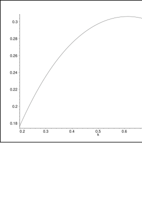
Figure 5: Dispersion as function of $k$

A minimal dispersion will be at $p=0.6$. This is the true value of $p$ because this value corresponds to the sense of minimal work. Dispersion will be

$$D^{\infty}=2\tilde{N^{\infty}}0.66229$$

We shall make our result more precise. We see that $\beta_{1}$ and $\beta_{2}$ are the first two terms of some series. We don’t know other terms, but it is reasonable to suppose that this series resembles geometric progression with denominator $\beta_{2}/\beta_{1}$. This leads to dispersion

$$D^{\infty}=2\tilde{N^{\infty}}0.64107$$

As it follows from fig.6 the value of extremum remains $p=0.6$

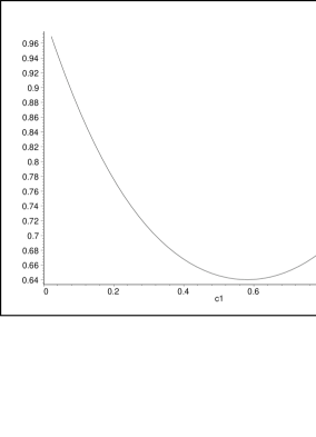
Figure 6: Dispersion as function of $c1\equiv p$

An absence of extremum shift is important and is necessary for this approach to be a self consistent.

Now we shall make the value of dispersion more accurate Due to the similarity of nucleation the first cycle doesn’t differ from the whole period. Function $\beta$ for the first cycle will be

$$\beta=\beta_{1}-\beta_{2}$$

$$\beta_{1}=8\int_{p_{1}}^{p}d\xi\int_{0}^{p_{1}}d\tau(\xi-\tau)^{3}\exp(-\xi^{4})$$

$$\beta_{2}=16\int_{p_{1}}^{p}d\xi\int_{p_{1}}^{p}d\eta\int_{0}^{p_{1}}d\tau(\tau-\xi)^{3}(\tau-\eta)^{3}\exp(-\xi^{4})\exp(-\eta^{4})$$

Calculations for $p_{1}=0.6*0.6=0.36$ and $p=0.6$ give $\beta=0.0255$.

Now we shall reconstruct $\beta_{eff}$ based on $D^{\infty}_{2}=2\tilde{N^{\infty}}0.64107$ We have $\beta_{eff}=(1-D^{\infty}/\tilde{N^{\infty}})/\alpha$ where $\alpha=0.9092$. Calculations give $\beta_{eff}=0.3268$. One has to add $\beta=0.0255$ which leads to $\beta=0.35156$. For this value of $\beta$ the value of dispersion will be

$$D^{\infty}_{3}=2\tilde{N^{\infty}}0.61332$$

This is our final result.

When we consider the dispersion which differs from $D^{\infty}_{0}=2\tilde{N^{\infty}}$ we have the shift of result

$$\delta D=D^{\infty}_{3}-D^{\infty}_{2}$$

This shift has to lead to a variation of dispersion in a fist cycle and to a variation of the total dispersion. Having linearized this effect we get to the final value of dispersion

$$D_{4}^{\infty}=D_{2}^{\infty}+\delta D\frac{D_{2}^{\infty}}{D_{3}^{\infty}}$$

and after calculations

$$D^{\infty}_{3}=2\tilde{N^{\infty}}0.62309$$

This value practically coincides with the previous value.

Another way to make results more precise is take into account the shift of dispersion directly in initial formulas. Having written for the dispersion correction in the first cycle

$$D^{\infty}_{3}=2\tilde{N^{\infty}}\gamma$$

with parameter $\gamma$, we get for the final distribution

$$P^{(k)}(M^{(k)}\sim\int_{\infty}^{\infty}dN_{1}dN_{2}...dN_{P}\prod_{i=1}^{P}\exp(-\frac{(N_{i}-\bar{N_{1}})^{2}}{2\gamma\bar{N_{1}}})$$

$$\exp[\frac{[N^{(k)}-\tilde{N^{(k)}}-\sum_{j=1}^{P}a_{j}(N_{j}-\bar{N_{j}})]^{2}}{2(\tilde{N^{(k)}}-P\bar{N_{1}})}]$$

where $P$ is the number of elementary intervals until argument $p$, $\tilde{N^{(k)}}$ is the number of droplets calculated on the base of the theory with averaged characteristics, $\bar{N_{i}}$ the mean number of droplets formed during interval number $i$ with account of fluctuations from previous intervals. The values $a_{i}$ are given by

$$a_{i}=1-\sum_{j=P+1}^{k}\frac{\exp(-j^{4}/M^{4})}{M^{4}}4(j-i)^{3}$$

and $M$ is the total number of intervals.

Having fulfilled integration $\int_{\infty}^{\infty}dN_{1}dN_{2}...dN_{P}$, we get for a limit value of dispersion

$$D^{\infty}=2\tilde{N^{\infty}}(1-\frac{p(1-\gamma)}{\alpha}-\frac{\gamma\beta}{\alpha})$$

which leads to equation on $\gamma$, which can be easily solved

$$\gamma=\frac{1-\frac{p}{\alpha}}{1+\frac{\beta}{\alpha}-\frac{p}{\alpha}}$$

Calculations lead to

$$\gamma(p=0.6)=0.5083$$

This result is very strange. It radically differs from the previous one. The reason of an error is that the duration of the first cycle is limited by $p$. So, we have to limit the duration of a whole period. The limit is, evidently, $\sim 1$. So, we have to recalculate $\beta$ as

$$\beta=\beta_{1}-\beta_{2}$$

$$\beta_{1}=8\int_{p}^{1}d\xi\int_{0}^{p}d\tau(\xi-\tau)^{3}\exp(-\xi^{4})$$

$$\beta_{2}=16\int_{p}^{1}d\xi\int_{p}^{1}d\eta\int_{0}^{p}d\tau(\tau-\xi)^{3}(\tau-\eta)^{3}\exp(-\xi^{4})\exp(-\eta^{4})$$

Now we shall show a dependence $\beta_{initial}$ on $p$ at fig. 7.

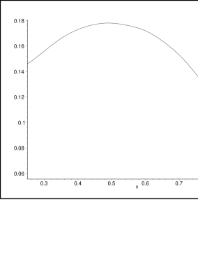
Figure 7: $\beta_{initial}$ as a function of $p$

Calculations give $\beta_{initial}=0.17$ and for the final dispersion

$$D^{\infty}_{3}=2\tilde{N^{\infty}}0.6436$$

This value coincides with a previous approach. It can be made more accurate by a geometric progression summation spoken above.

3 Numerical results

Numerical simulation of nucleation can be done by the following method. We split the nucleation interval into many parts (steps). At every step a droplet will be formed or not. The probability to appear must be rather low, then we have the smallness of probability to have two droplets at the same interval. This means that the interval is ”elementary”.

The process of formation is simulated by a random generator in a range $[0,1]$. If a generated number is smaller than a threshold parameter $u$, then there will be no formation of a droplet. If it is greater than a threshold, we shall form a droplet. As a result we have spectrum $\hat{f}$ of droplets sizes. Now it is a chain of $0$ and $1$. The parameter $u$ descends according to macroscopic law

$$u=u_{0}\exp(-\Gamma G/\Phi)$$

from a theory with averaged characteristics (it is based only on a conservation law without any averaging and can be used). Here

$$\Gamma=\frac{dF_{c}}{d\Phi}\sim\nu_{c}$$

$\Phi$ is the initial supersaturation, $F_{c}$ is a free energy of critical embryos formation, $\nu_{c}$ is a number of molecules inside a critical embryo, $G$ is the number of molecules in a new phase taken in units of a molecules number density in a saturated vapor. By renormalization one can take away all parameters except $G$.

To simplify calculations radically one can use the following representation [6] for $G$:

$$G=z^{3}G_{0}-3z^{2}G_{1}+3zG_{2}-G_{3}$$

where $z$ is a coordinate of a front of spectrum, and $G_{i}$ are given by

$$G_{i}=\int_{0}^{z}\hat{f}(x)x^{i}dx$$

We needn’t to recalculate $G_{i}$, but can only ascend the region of integration, having added to integrals $z^{i}\hat{f}(z)dx$ at every step.

Our results are given below. The interval is split into $30000$ parts. Parameter $u_{0}$ have been varied from $0$ up to $1$ which leads to a different number of droplets. It is clear that the limit values are not good: at $0$ there are no droplets in the system, at $1$ our intervals are not elementary. At every $u_{0}$ results were averaged over $1000$ attempts.

Shifts of droplets numbers are drawn at fig.8 as a function of $\ln\tilde{N^{(\infty)}}$

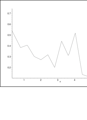
Figure 8: Shifts of droplets numbers as a function of $\ln\tilde{N^{(\infty)}}$

It is seen that an analytical result about negligible value of corrections is correct.

Dispersion as a function of $\ln\tilde{N^{(\infty)}}$ is shown at fig. 9.

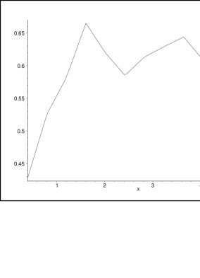
Figure 9: $\gamma$ as a function of $\ln\tilde{N^{(\infty)}}$

It is seen that analytical value of dispersion coincides with numerical simulation. The ends of the curve correspond to a zero number of droplets and to a giant number of droplets when the elementary intervals are not elementary and have to be thrown out.

Stochastic effects in dynamic conditions [6] can be analyzed by the same method. We needn’t to describe it here. Numerical results are drawn below. Fig. 10 shows the shift in the number of droplets. It is small. Dispersion is drawn at fig. 11 (i.e. the value of $\gamma$). It is greater than in the case of decay.

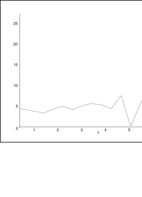
Figure 10: Shift in a droplets number as a function of $\ln\tilde{N^{(\infty)}}$ for dynamic conditions

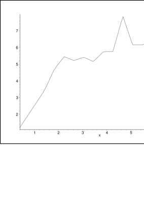
Figure 11: $\gamma$ as a function of $\ln\tilde{N^{(\infty)}}$ for dynamic conditions

The physical reasons for the smallness of the droplet number shift for decay and for dynamic conditions will be different.

For decay the reason is the following. The system wait the first droplet as long as necessary. Actually the time for kinetics of this system is $t(G)$ with no connection with real time (certainly, the rate of nucleation has such connection). This phenomena is the reason for a smallness.

In dynamic conditions there is a time dependent parameter - the intensity of external source. So, there is no such a reason.

But here in the theory with averaged characteristics there is a property of a weak dependence on microscopic corrections for a free energy [6]. The same is valid also for fluctuation deviations. So there will be a weak effect of stochastic nucleation.

Because the reasons for smallness of effect in decay and dynamic conditions are different it is interesting to see whether they continue to act when supersaturation is stabilized at some moment. Analytical results shows that the will be an overlapping of two reasons.

Really, if stabilization takes place at the period where the main consumers of vapor are going to appear then the majority of droplets appear in the situation when there is no influence on the system. Then the situation for these droplets resembles decay conditions (and may be even better because the external supersaturation [3] is going to decrease). So the reason for the decay situation works here.

If stabilization takes place at the second cycle, then the behavior of supersaturation is governed by droplets formed in dynamic conditions and we have here the reason for smallness in dynamic conditions. In both situations the effect is small. Numerical results confirm this conclusion.

The main result of this publication is a correct definition of all main characteristics of stochastic nucleation. It is shown that the main role in stochastic effects belongs to all droplets, but not to the main consumers of vapor. Only the property of the nucleation conditions similarity allows us to solve the problem of account of all influences during the nucleation period.

When all disadvantages of [1], [2] are shown it is clear that these theories can not be considered as a solid base for nucleation investigation.

But why results obtained in [1], [2] are so close numerically to real values. The reason is that on a level of averaged characteristics there is a universality of nucleation process. So, the errors of [1], [2] cannot lead to a qualitatively wrong results.

One has to stress that all corrections obtained in this paper are also universal ones. Certainly, they are some coefficients in decompositions and the functional form is prescribed now (contrary to the theory with averaged characteristics).

It seems that all effects considered here are negligible. For simple systems it is really true. But for systems with more complex kinetic behavior these effects can be giant. One of such systems is already described theoretically and this description will be presented soon in a separate publication.

In diffusion regime of droplets growth one has to use another approach based on [8], [7]. In [7] an explicit description of nucleation with account of stochastic effects was constructed.

A nucleation with growing volumes of interaction will be presented in the next paper.

References

- [1] Grinin A.P., F.M.Kuni, A.V. Karachencev, A.M.Sveshnikov Kolloidn. journ. (Russia) vol.62 N 1 (2000), p. 39-46 (in russian)
- [2] Grinin A.P., A.V. Karachencev, Ae. A. Iafiasov Vestnik Sankt-Peterburgskogo universiteta (Scientific journal of St.Petersburg university) Series 4, 1998, issue 4 (N 25) p.13-18 (in russian)
- [3] Kurasov V.B. Universality in kinetics of the first order phase transitions. Chemistry research Institute of St.Petersburg State University. St.Petersburg, 1997, 400 p.
- [4] Kurasov V.B. Development of the universality conception in the first order phase transitions. Chemistry research Institute of St.Petersburg State University. St.Petersburg, 1998, 125 p.
- [5] Kurasov V.B. Manuscript published in VINITI 2594 95 from 19.09.95, 28 p. (in russian)
- [6] Kurasov V.B. Phys.Rev.E vol. 49, p. 3948 (1994)
- [7] Kurasov V.B. Heterogeneous condensation in dense media, Phys.Rev.E Vol 63, 056123, (2001)
- [8] Kurasov V.B., Physica A vol.226, p.117 (1996)